國
立
交
通
大
學
多媒體工程研究所
碩
士
論
文
在光源及視點空間最佳重新參數化的雙向
貼
圖
函
數
模
型
Bidirectional Texture Function Modeling Using
Optimized Reparameterization in the Lighting and
Viewing Space
研 究 生:方奎力
指導教授:林文杰 教授
Bidirectional Texture Function Modeling Using Optimized
Reparameterization in the Lighting and Viewing Space
Student: Kuei-Li Fang
Advisor: Dr. Wen-Chieh Lin
Institute of Multimedia Engineering
College of Computer Science
National Chiao Tung University
ABSTRACT
We present a new approach to model BTF data using multivariate SRBF kernels. More impor-tantly, we propose a data-dependent reparameterization method in which optimal reparameteri-zation in the lighting and viewing space that minimizes the modeling error is obtained. To speed up our BTF modeling computation and improve spatial coherence of acquired BTF model, we utilize a mipmap hierarchy in our BTF model, which can be nicely integrated with graphics hardware when rendering BTF data. Our experiments show that the optimal reparameterization does provide better accuracy than a fixed reparameterization such as the half-way reparameter-ization. In addition, real-time rendering of BTF from novel viewing or lighting direction that is not recorded in the original BTF database can be achieved easily.
Acknowledgments
I would like to thank Ph.D. Candidate Yu-Ting Tsai who provides the idea of optimal repa-rameterization and helpful suggestions on implementation. I also want to thank my advisors Dr. Wen-Chieh Lin who gives me a lot guidance, inspirations, useful ideas, and teach me the attitude of hard-working. Thanks to my colleagues: Shang-Wen Wang, Wei-Chien Cheng, Chin-Hsian Chang, Yueh-Tse Chen, Hsin-Hsiao Lin, Tsung Li, Zhi-Han Yan, Ming-Shang Hsu, Ying-Shou Lan, and Jia-Ru Lin for their assistances and discussions. It is honor to work with all of you. At last, I would like to thank my parents for their unselfish love and support.
Contents
1 Introduction 1 2 Previous Work 4
2.1 Bidirectional Texture Function . . . 4
2.2 Reparameterization of Reflectance Functions . . . 5
2.3 Modeling of Reflectance Data . . . 5
3 Approach 7 3.1 Overview . . . 7 3.2 Background . . . 9 3.2.1 Multivariate SRBF . . . 9 3.2.2 Optimal Reparameterization . . . 11 3.3 Implementation Issues . . . 11 3.3.1 Initial Guess . . . 12 3.3.2 Mipmap Construction . . . 13
3.3.3 Multi-resolution Optimal Repameterization . . . 13
3.3.4 Smooth Terms . . . 14
3.3.5 Optimization . . . 15
3.3.6 Rendering System . . . 15
4 Results 16
4.1 Data Acquisition . . . 16
4.2 Univariate SRBF vs. Multivariate SRBF . . . 16
4.3 Half-way Reparameterization vs. Optimal Reparameterization . . . 19
4.4 Smooth terms vs. No Smooth terms . . . 24
4.5 Time Consumption and Compression Ratio . . . 26
4.6 Rendering Results . . . 26 5 Conclusion and Future Work 30 Bibliography 32
List of Figures
3.1 Approach Overview . . . 8 3.2 Comparison of BTF data and representation by Gaussian SRBFs and
multi-variate Gaussian SRBFs. (a)(b) are textures of corduroy data from Bonn BTF database. (c)(d) are reconstructed results by multivariate Gaussian SRBFs via half-way reparameterization. (e)(f) are reconstructed results by Gaussian SRBFs. Twenty SRBF kernels(J = 20) are used in (c)(d)(e)(f), Three multivariate modes(K = 3) are used in (c)(d). . . 10 3.3 We propagate $ of mipmap level l+1 to mipmap level l . . . 14 3.4 (a)(b) are rendering results without and with smooth terms. Yellow sphere is
the point light source located above the right side of mesh. . . 14 4.1 RMS error comparison of univariate SRBF and multivariate SRBF; X-axis is
mipmap level and Y-axis is RMS error . . . 17 4.2 Reconstructed results comparison of univariate SRBF and multivariate SRBF.
(a)(b)(c)(d) are textures of corduroy and wool data from Bonn BTF database, re-spectively. (e)(f)(g)(h) are reconstructed results using Gaussian SRBFs via opti-mal reparameterization. (i)(j)(k)(l) are reconstructed results using multivariate Gaussian SRBFs via optimal reparameterization. Twenty SRBF kernels(J = 20) are used in (e)(f)(g)(h)(i)(j)(k)(l), three multivariate modes(K = 3) are used in (i)(j)(k)(l). . . 18
4.3 RMS error comparison of representation results using our optimal reparameter-ization and half-way reparameterreparameter-ization; X-axis is mipmap level and Y-axis is RMS error . . . 19 4.4 Reconstructed results comparison of our optimal reparameterization and
half-way reparameterization. (a)(b) are textures of corduroy data from Bonn BTF database. (d)(e) are reconstructed results using our optimal reparameterization. (h)(i) are reconstructed results using half-way reparameterization. (c)(f)(g)(j) are error images of (d)(e)(h)(i) compare to (a)(b)(a)(b) respectively. Twenty multivariate SRBF kernels (J = 20) and three multivariate modes (K = 3) are used in (d)(e)(h)(i). The RMS error of (d)(e)(h)(i) are 0.049926, 0.047594, 0.057197, 0.04814 respectively. . . 20 4.5 Reconstructed results comparison of our optimal reparameterization and
half-way reparameterization. (a)(b) are textures of ceiling data from Bonn BTF database. (d)(e) are reconstructed results using our optimal reparameterization. (h)(i) are reconstructed results using half-way reparameterization. (c)(f)(g)(j) are error images of (d)(e)(h)(i) compare to (a)(b)(a)(b) respectively. Twenty multivariate SRBF kernels(J = 20) and three multivariate modes(K = 3) are used in (d)(e)(h)(i). The RMS error of (d)(e)(h)(i) are 0.029616, 0.040331, 0.032102, 0.042219 respectively. . . 21 4.6 Reconstructed results comparison of our optimal reparameterization and
half-way reparameterization. (a)(b) are textures of Impalla data from Bonn BTF database. (d)(e) are reconstructed results using our optimal reparameterization. (h)(i) are reconstructed results using half-way reparameterization. (c)(f)(g)(j) are error images of (d)(e)(h)(i) compare to (a)(b)(a)(b) respectively. Twenty multivariate SRBF kernels(J = 20) and three multivariate modes(K = 3) are used in (d)(e)(h)(i). The RMS error of (d)(e)(h)(i) are 0.060246, 0.064558, 0.063839, 0.081254 respectively. . . 22
4.7 Rendering results comparison of wool using optimal reparameterization and half way reparameterization. Twenty multivariate SRBF kernels(J = 20) and three multivariate modes(K = 3) are used. . . 23 4.8 Rendering results comparison of impalla using optimal reparameterization and
half way reparameterization. Twenty multivariate SRBF kernels(J = 20) and three multivariate modes(K = 3) are used. . . 23 4.9 Rendering results comparison of corduroy without smooth terms and with smooth
terms. Twenty multivariate SRBF kernels(J = 20) and three multivariate modes(K = 3) are used. . . 24 4.10 Reconstructed results comparison of our optimal parameter BTF model with
smooth terms and without smooth terms. (a)(b)(c) are textures of corduroy data from Bonn BTF database. (d)(e)(f) are reconstructed results with smooth terms. (g)(h)(i) are reconstructed results without smooth terms. Twenty multivariate SRBF kernels (J = 20) and three multivariate modes (K = 3) are used in (c)(d)(e)(f)(g)(h)(i). . . 25 4.11 Rendering result of wool with optimal reparameterization. (J=20,K=3) . . . 27 4.12 Rendering result of corduroy with optimal reparameterization. (J=20,K=3) . . . 28 4.13 Rendering result of ceiling with optimal reparameterization. (J=10,K=3) . . . . 28 4.14 Rendering result of ceiling with optimal reparameterization. (J=10,K=3) . . . . 29
List of Tables
4.1 Elapsed time of BTF modeling. J and K denote number of multivariate SRBF kernels and number of multivariate modes. . . 26 4.2 Data size of data in BTF database Bonn. All textures are stored with JPEG format 27 4.3 Data size of our BTF modeling. J and K denote number of multivariate SRBF
kernels and number of multivariate modes. . . 27 4.4 FPS of rendering. J and K denote number of multivariate SRBF kernels and
number of multivariate modes. . . 29
C H A P T E R
1
Introduction
Rendering materials with complex meso structures and reflectance behaviors used to be a great challenge in computer graphics. It is hard to describe reflectance behavior with simple an-alytic models, so recent rendering algorithms synthesize high-quality images from precomputed results or measured reflectance data. These image-based rendering algorithms have tremendous advances over the last decades. Dana et al.[4] introduced the bidirectional texture function (BTF) to model the appearance of materials in different viewing and lighting directions. A BTF is a 6D function that stores spatially-varying reflectance appearance of materials. Therefore, images rendered from measured BTFs can faithfully exhibit complex lighting effects and de-tailed meso-structures of real-world objects, including the micro-geometry of rough surfaces, self-shadows, and multiple light scattering.
As BTF is a collection of discrete texture data with enormous data size, how to efficiently compress and model BTF data is a great challenge. This challenge has stimulated recent devel-opment of approximation algorithms for large-scale surface appearance models[1, 3, 4, 6, 11]. The appearance of a BTF depends on various physical parameters. This high-dimensional data is too complicated to be presented by a simple analytic model, so we introduce a sum-of-product model to describe complex anisotropic reflectance behaviors of BTF data. More specifically,
2 we decompose a reflectance field as a linear combination of multivariate spherical radial basis functions (SRBFs), while each multivariate SRBF is constructed from the product of univariate SRBF1.
Transforming the parameters of a reflectance function into another parametric space, which we called reparameterization[7, 11, 17, 21] is a well-known method to improve approximation efficiency; however, only fixed function reparameterization was introduced in previous articles. In this thesis, we propose a data-dependent reparameterization method. We propose to find the optimized reparameterization function, so we use a parametric representation in viewing and lighting space to model the BTF data and integrate parameters optimization into our frame-work. Fixed functions reparameterization, such as half-way vector becomes special cases in our general framework.
In order to exploit spatial coherence in BTF data more efficiently, we also utilize the mipmap hierarchy in our framework. We find the optimized representation of the highest level in mipmaps at first, then propagate results from higher level to lower level. As a result, we can make our optimization process much faster and still remain great quality. With this hierarchy, hardware support such as mipmaps can also been used at run time stage.
The contributions of this thesis can be summarized as:
• A novel functional representation based on the linear combination of multivariate spher-ical radial basis functions is introduced to accurately model the anisotropic behavior of measured reflectance fields.
• An automatic reparameterization framework is proposed to learn the best parameter trans-formation function from a given reflectance data set.
• A multi-scale optimization algorithm for spatially-varying materials is presented to ex-ploit the spatial coherence among data and accelerate the approximation process.
The rest of this thesis is organized as follows: Chapter 2 reviews previous methods for
3 modeling surface reflectance. Chapter 3 illustrates the proposed algorithm for modeling BTF. Chapter 4 shows our experimental results. In the end, conclusion and future work are discussed in Chapter 5.
C H A P T E R
2
Previous Work
In this section, we give an brief introduction of BTF in section 2.1, then review some repa-rameterization methods in section 2.2 and recent approximation algorithms for reflectance fields in section 2.3
2.1
Bidirectional Texture Function
BTF is a 6D function T (x, y, ηi, ηo) = T (x, y, θi, φi, θo, φo) proposed by Dana et al.[4],
where x, y, θi, φi, θo, φo denote the spatial coordinates, illumination and view directions in
spherical coordinate, respectively. The BTF data is a set of images taken from different illumi-nation and view directions. Without regard to spatial dimensions, we can take BTF as ordinary reflectance function such as BRDF ρ(θi, φi, θo, φo).
Due to enormous data size of BTF, how to compress and model BTF becomes an important issue in BTF manipulation. Recent researches focus on recovering ways to model these BTF data. Vasilescu and Terzopoulos[1] organized BTF textures as a tensor, and then extracted basis matrices in each mode by traditional PCA. Wang et al.[20] also proposed an out-of-core and
2.2 Reparameterization of Reflectance Functions 5 block-wise tensor by using an optimal N-mode SVD algorithm. These dimensionality reduction techniques still need to use interpolation between each basis to fill the hole between sparsely observed view and lighting directions and only allowing one of lighting or viewpoint variation. Zickler et al.[21] modeled spatially-varying BRDFs as continuous RBF functions via half-way reparameterization[17]; However, Szymon[17] assumed the BRDF model are isotropic, so half-way reparameterization is not suitable for modeling anisotropic reflectance behaviors. In our work, we propose a BTF model reparameterized by optimal parameters in illumination and view space.
2.2
Reparameterization of Reflectance Functions
Reflective[16] and half-way[17] reparameterization for BRDFs are well-known methods to model highly specular materials. Recently, Lawrence et al.[11] and Zickler et al.[21] applied these reparameterization to approximate spatially-varying BRDFs. In general, reparameteri-zation is beneficial reducing the dimensionality and greatly increasing the data coherence of reflectance functions.
Previous reparameterization techniques are limited to fixed or heuristic transformation func-tions; however, it is unknown which parameter transformation is suitable for the reflectance data. In this thesis, we propose to find the optimized reparameterization function from data, with restricted functional forms.
2.3
Modeling of Reflectance Data
Modern approximation algorithms for reflectance fields can be summarized into two main categories: non-parametric models and functional linear models.In non-parametric models, an appropriate basis is learnt from data for an accurate representation rather than pre-defined ba-sis functions. Clustering and dimensional reduction techniques are the most popular methods in computer graphics, e.q. matrix factorization[11, 14], principal component analysis[3, 8, 18],
2.3 Modeling of Reflectance Data 6 tensor approximation[1, 20] and vector quantization[13]. Although non-parametric methods are entirely data-driven models that yield accurate and flexible representations, the compressed data is still huge; It is difficult to render BTF in real time with non-parametric models. Also, interpo-lation methods are still needed when rendering BTF from novel illumination and view direction. In contrast to non-parametric models, our method provides not only higher compression ratios but also real-time rendering performance under similar image quality; Our reparameterization function can represent reflectance data into continuous functions, so interpolation is not needed in our method.
The main concept of functional linear models is to expand a radiance function as a sum of pre-defined basis functions. The choice of an appropriate basis significantly influences render-ing performance and image quality. Previous articles have described reflectance fields usrender-ing parametric kernels[6, 9], radial basis functions[21], spherical harmonics[16], and wavelets[2]. In general, kernel and radial basis functions provide better run-time performance and quality for all-frequency materials. However, they usually require computationally expensive non-linear optimization for parameter estimation, which becomes even awful and impractical when model-ing BTF; In this thesis, we adopt the mipmap hierarchy and the expectation maximization(EM) algorithm in our framework to accelerate the non-linear optimization.
C H A P T E R
3
Approach
This chapter describes our algorithm. First, we give an overview of our approach in sec-tion 3.1. Next, we describe the background of our algorithm(secsec-tion 3.2), including multi-variate SRBF(section 3.2.1), optimal reparameterization(section 3.2.2). At last, we introduce our implementation issues(section 3.3), including mipmap construction(section 3.3.1), fitting with mipmap hierarchy(section 3.3.2), smooth terms(section 3.3.3), and our rendering system (section 3.3.4).
3.1
Overview
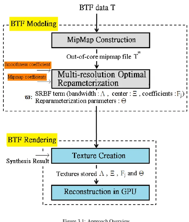
Figure 3.1 shows an overview of our approach, which consists of BTF modeling and BTF rendering.
T (x, y, ηi, ηo) (3.1)
A BTF is a 6D function T (x, y, ηi, ηo), where x and y denote the spatial coordinates and ηi and
ηo denote the illumination and view directions. Finding multivariate SRBF expansion of BTF
data with optimal parameters is the main task in BTF modeling. 7
3.1 Overview 8
Figure 3.1: Approach Overview
We first represent the input BTF T (x, y, ηi, ηo) as mipmap format Tl(x, y, ηi, ηo) where l
denotes the mipmap level, and T0(x, y, η
3.2 Background 9 structure, width and height of level k + 1 is half of level k.
In mipmap hierarchy fitting, we optimize coefficient, center, bandwidth of SRBF kernel and Θ of reparameterization function using the gradient-decent method; We find the optimal result of higher level in mipmap and propagate them to lower level until all levels are obtained.
We construct mipmap textures stored representation results and throw these textures into GPU memory. At BTF rendering stage, we compute illumination direction ηiand view direction
ηoat each pixels, and reconstruct BTF T by looking up the computed BTF model.
3.2
Background
We introduce background of our approach in this section. In section 3.2.1, we introduce Multivariate SRBF which is the extend form of the original SRBF introduced by Tsai and Shih[19]. In section 3.2.2, we introduce our optimal reparameterization method.
3.2.1
Multivariate SRBF
SRBFs[19] are circularly axis-symmetric functions defined on the unit sphere Sm. Let η and
ξ be two points on Sm, and θ be the geodesic distance between η and ξ, i.e. θ = arccos(η · ξ),
then a univariate SRBF is defined as a function G(cosθ) = G(η · ξ). Here is an example of univariate SRBFs called Gaussian SRBF kernel:
GGau(η · ξ; λ) = eλ(η·ξ)e−λ, (3.2) where λ is bandwidth and ξ is center of the SRBF kernel. Similar to RBFs in Rm+1, a spherical function F (η) can be represented as
F (η) =
n
X
j=1
FjG(η · ξj; λj) (3.3)
As BTF data is too complicate to be represented by univariate SRBFs, we combine sum-of-product of univariate SRBFs to form multivariate SRBFs. An example of multivariate SRBFs
3.2 Background 10 using the Gaussian SRBF kernel is listed below:
GM −Gau({ηk· ξk; λk}Kk=1) = e
P
kλk(ηk·ξk)−λk (3.4)
We use multivariate Gaussian SRBF kernel to model a spherical function F (η) as shown in Equation 3.5, where J is the number of multivariate Gaussian SRBF kernels and K is number of variables in multivariate Gaussian SRBF kernel.
F (η) = J X j=1 FjGM −Gau({ηk· ξj,k; λj,k}Kk=1); (3.5) (a) (b) (c) (d) (e) (f)
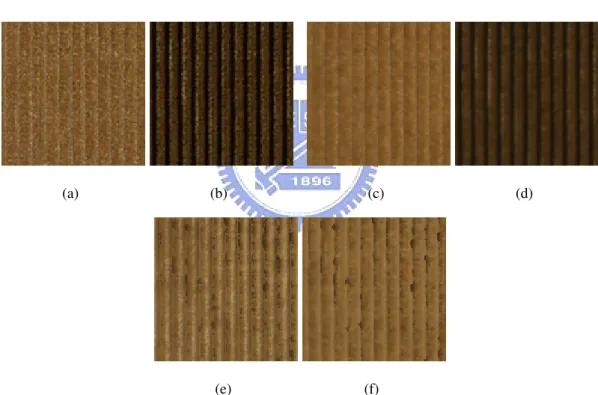
Figure 3.2: Comparison of BTF data and representation by Gaussian SRBFs and multivariate Gaussian SRBFs. (a)(b) are textures of corduroy data from Bonn BTF database. (c)(d) are reconstructed results by multivariate Gaussian SRBFs via half-way reparameterization. (e)(f) are reconstructed results by Gaussian SRBFs. Twenty SRBF kernels(J = 20) are used in (c)(d)(e)(f), Three multivariate modes(K = 3) are used in (c)(d).
3.3 Implementation Issues 11
3.2.2
Optimal Reparameterization
Reparameterization is a popular method in improving approximation efficiency. Let T (ηi, ηo)
be a BTF data without spatial varying, where ηi and ηodenotes the illumination directions and
view directions. We would like to find an optimized reparameterization function ψ(ηi, ηo|Θk),
with parameter set Θk, such that another function F (ψ(ηi, ηo|Θk)) can approximates T (ηi, ηo)
efficiently.
As mention above, we can model T (ηi, ηo) using multivariate Gaussian SRBF kernel as
follows: T (ηi, ηo) = F (ψ(ηi, ηo|Θk)) = J X j=1 FjGM −Gau({ψ(ηi, ηo|Θk) · ξj,k; λj,k}Kk=1) (3.6)
In this work, we use a linear combination form showed below as our reparameterization trans-form function.
ψ(ηi, ηo|Θk) = akηi+ bkηo (3.7)
We define our objective function Eb below:
Eb = X ι,υ (T (ηiι, ηoυ) − J X j=1 FjGM −Gau({ψ(ηιi, η υ o|Θk) · ξj,k; λj,k}Kk=1))2 (3.8)
Then, we optimize Θk using this objective function Eb until we get the optimal transfer
function.1
3.3
Implementation Issues
In this section, we describe issues when we implement our method. First, We introduce how we get a proper initial guess(section 3.3.1) and how we construct mipmap file of BTF data(section 3.3.2), then how to model BTF data with mipmap hierarchy(section 3.3.3) and how to smooth our BTF model in spatial dimension(section 3.3.4) is followed, at last, rending part(section 3.3.5) including reconstructed results and texture synthesis is listed.
1We use ’L-BFGS’(http://www.alglib.net/optimization/lbfgs.php) which is a software package for solving
3.3 Implementation Issues 12
3.3.1
Initial Guess
As our optimization problem involves many high-dimensional variables, a good initial is important. We adopt standard expectation maximization(EM) algorithm to obtain an initial guess for our optimization problem. This is based on the assumption that each SRBF kernel is independent. As this assumption does not hold when using SRBF to model BTF, we only use EM to obtain the initial guess.
In the E step, we evaluate a probability density function P defined as follows: P ((j, k)|ψ(ηiι, ηoυ|Θk), Ξ, Λ) = FjGM −Gau(ψ(ηiι, ηυo|Θk) · ξj,k; λj,k) PJ j=1FjGM −Gau({ψ(ηiι, ηoυ|Θk) · ξj,k; λj,k} K k=1) (3.9) where ηι
i and ηoυare respectively the ι-th illumination direction and the υ-th view direction and
Ξ and Λ are sets of SRBF centers ξj,k and bandwidth λj,k.
In the M step, we maximize the exception value Q as follows: Q =X ι,υ J X j=1 K X k=1 λj,kT (ηiι, η υ o)(ψ(η ι i, η υ o|Θk) · ξj,k)P ((j, k)|ψk(ηiι, η υ o|Θk), Ξ, Λ) (3.10)
If we assume that the distribution P is fixed when optimizing Θk, Equation 3.10 can be further
simplified into Q =X ι,υ J X j=1 K X k=1 λj,kT (ηiι, ηυo)(ψ(ηιi, ηoυ|Θk) · ξj,k)P ((j, k)|ηιυ, Ξ, Λ) (3.11)
where ηιυis the reparameterized direction of ηiιand ηoυin previous iteration. Traditional
gradient-based non-linear optimization process then can be applied to update Θk.
After we get Θkfrom EM step, we can take the result into objective function Ebin Equation
3.3 Implementation Issues 13
3.3.2
Mipmap Construction
When a BTF data first into our system, we construct mipmap data of each BTF textures using Lanczos resampling[5], the Lanczos filter is defined below:
L(x) = asin(πx)sin(π ax) π2x2 , −a < x < a, x 6= 0 1, x = 0 0, otherwise. (3.12) Where a is set to be three in our method. We store the BTF mipmap data into an out-of-core three dimensional array. The first dimension is the mipmap level from highest level(contains only one texel) to lowest level(original texture size); The second dimension is spatial dimension according to the position of textel in the texture; The third dimension is illumination and view directions.
3.3.3
Multi-resolution Optimal Repameterization
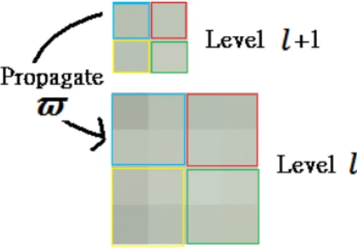
Let $(x, y, l) be the BTF model parameters which contains scale coefficients Fjand centers
ξ and bandwidths λ of SRBF kernels and reparameterization parameters θ in spatial position (x, y) of mipmap level l. As Figure 3.3 shows, we use $(x/2, y/2, l) as the initial guess to find optimized $(x, y, l + 1). To keep $ varying slowly when mipmap level changes, we set a mipmap constrain Em showed in Equation 3.13 into our objective function Eb in Equation 3.8,
where cmip is the weight of mipmap constrain. Our method ensures $ change slightly when
mipmap level changes, so we can use hardware acceleration to smooth mipmap level switch and still remain great quality.
Em = cmip∗
X
x,y,l
3.3 Implementation Issues 14
Figure 3.3: We propagate $ of mipmap level l+1 to mipmap level l
3.3.4
Smooth Terms
To assure rendering quality, SRBF and reparameterization coefficients need to be continuous in spatial domain. We enforce the spatial smoothness constrains Es on the SRBF coefficients
and reparameterization parameters: Es= cSmooth∗ X x,y,l 2 X dx=−2 2 X dy=−2 ($(x, y, l) − $(x + dx, y + dy, l))2, (3.14) where cSmoothis used to control the weights of neighbor differences in objective functions.
(a) (b)
Figure 3.4: (a)(b) are rendering results without and with smooth terms. Yellow sphere is the point light source located above the right side of mesh.
3.3 Implementation Issues 15
3.3.5
Optimization
Combining Equations 3.8 3.13 3.14, we have an objective function E:
E = Eb+ Em+ Es (3.15)
We use the limited memory Broyden-Fletcher-Goldfarb-Shanno(BFGS) method supported by a software package called L-BFGS(from http://www.alglib.net/optimization/lbfgs.php) to solve this optimization problem.
3.3.6
Rendering System
In rendering part, we send result of BTF representation to GPU by mipmap textures. At run time, we derive illumination direction ηi and view direction ηo of each pixel and reconstruct
the illumination result from Equation 3.5. As reconstruction is the bottleneck of rendering per-formance, we use smooth terms in representation stage to make SRBF and reparameterization coefficients continuous in spatial, so we can using texture filter from hardware support to do linear interpolation for SRBF and reparameterization coefficients.
To improve rendering quality, BTF synthesis is necessary. We use the method proposed by Lefebvre el at.[12] to synthesize BTF. We treat the original BTF data T (x, y, ηi, ηo) as
the appearance vector, and use the tensor approximation method to reduce the dimensions of T (x, y, ηi, ηo) and apply anisometric synthesis method mentioned in [12].
C H A P T E R
4
Results
4.1
Data Acquisition
All the BTF data are from BTF Database Bonn(http://btf.cs.uni-bonn.de/). The CORDUROY data and the IMPALLA data and the WOOL data consists of 6561 images, 256x256 resolution, 81 view and 81 light directions. The CEILING data consists of 6561 images, 800x800 resolu-tion, 81 view and 81 light directions, and we resample the CEILING data to 256*256 resolution using Lanczos filter.
4.2
Univariate SRBF vs. Multivariate SRBF
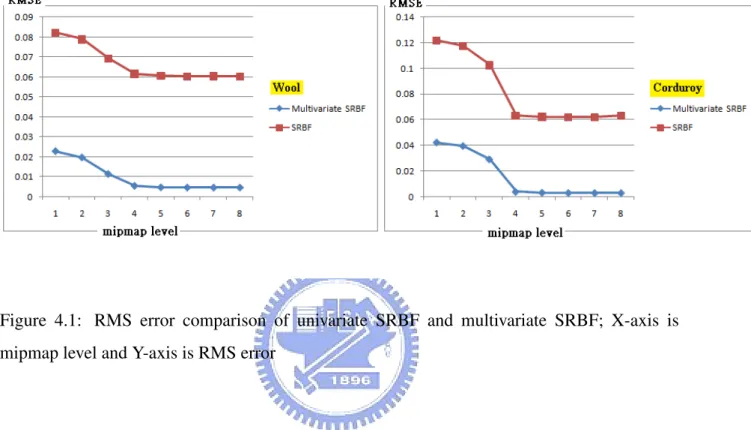
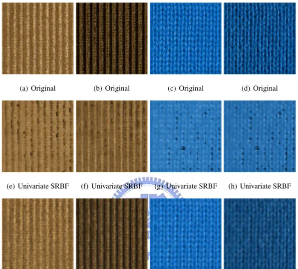
At first, we compare the results of our optimal parameterized BTF model using univariate SRBF and multivariate SRBF. Figure 4.1 shows the RMS error comparison of univariate SRBF and multivariate SRBF. We calculate RMS errors of reconstructed results in different resolution levels of the Mipmap data of original BTF data from all lighting and viewing directions. The reconstructed results are shown in Figure 4.2. Although BRDF data can be modeled efficiently using univariate SRBF in [19], it is difficult to model BTF data using univariate SRBF. One can
4.2 Univariate SRBF vs. Multivariate SRBF 17 observe that there is obvious error in univariate results Figure 4.2(e)(f)(g)(h) while the image quality is much better in multivariate SRBF results Figure 4.2(i)(j)(k)(l).
Figure 4.1: RMS error comparison of univariate SRBF and multivariate SRBF; X-axis is mipmap level and Y-axis is RMS error
4.2 Univariate SRBF vs. Multivariate SRBF 18
(a) Original (b) Original (c) Original (d) Original
(e) Univariate SRBF (f) Univariate SRBF (g) Univariate SRBF (h) Univariate SRBF
(i) Multivariate SRBF (j) Multivariate SRBF (k) Multivariate SRBF (l) Multivariate SRBF Figure 4.2: Reconstructed results comparison of univariate SRBF and multivariate SRBF. (a)(b)(c)(d) are textures of corduroy and wool data from Bonn BTF database, respectively. (e)(f)(g)(h) are reconstructed results using Gaussian SRBFs via optimal reparameterization. (i)(j)(k)(l) are reconstructed results using multivariate Gaussian SRBFs via optimal reparame-terization. Twenty SRBF kernels(J = 20) are used in (e)(f)(g)(h)(i)(j)(k)(l), three multivariate modes(K = 3) are used in (i)(j)(k)(l).
4.3 Half-way Reparameterization vs. Optimal Reparameterization 19
4.3
Half-way Reparameterization vs. Optimal
Reparameter-ization
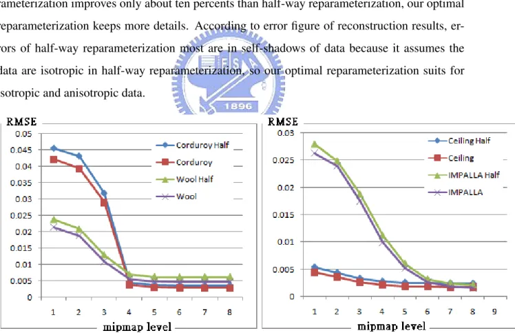
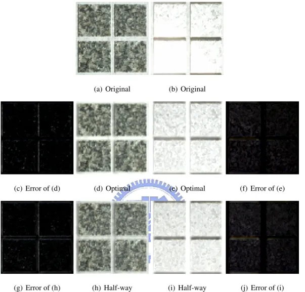
We show the improvement of our optimal reparameterization compared to half-way repa-rameterization. The RMS error comparison is listed in Figure 4.3 and the reconstructed results are showed in Figure 4.4 and Figure 4.5. These experiments are set with mipmap hierarchy and smooth terms, so the result would be smooth in spatial domain. As the ceiling BTF data have less height variation in different spatial position, the reflectance behavior is much simpler, and the RMS error is smaller than the others. Although the RMS error of our optimal repa-rameterization improves only about ten percents than half-way reparepa-rameterization, our optimal reparameterization keeps more details. According to error figure of reconstruction results, er-rors of half-way reparameterization most are in self-shadows of data because it assumes the data are isotropic in half-way reparameterization, so our optimal reparameterization suits for isotropic and anisotropic data.
Figure 4.3: RMS error comparison of representation results using our optimal reparameteriza-tion and half-way reparameterizareparameteriza-tion; X-axis is mipmap level and Y-axis is RMS error
4.3 Half-way Reparameterization vs. Optimal Reparameterization 20
(a) Original (b) Original
(c) Error of (d) (d) Optimal (e) Optimal (f) Error of (e)
(g) Error of (h) (h) Half-way (i) Half-way (j) Error of (i)
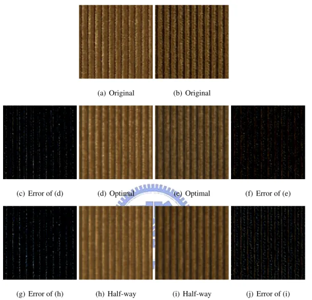
Figure 4.4: Reconstructed results comparison of our optimal reparameterization and half-way reparameterization. (a)(b) are textures of corduroy data from Bonn BTF database. (d)(e) are reconstructed results using our optimal reparameterization. (h)(i) are reconstructed results using half-way reparameterization. (c)(f)(g)(j) are error images of (d)(e)(h)(i) compare to (a)(b)(a)(b) respectively. Twenty multivariate SRBF kernels (J = 20) and three multivariate modes (K = 3) are used in (d)(e)(h)(i). The RMS error of (d)(e)(h)(i) are 0.049926, 0.047594, 0.057197, 0.04814 respectively.
4.3 Half-way Reparameterization vs. Optimal Reparameterization 21
(a) Original (b) Original
(c) Error of (d) (d) Optimal (e) Optimal (f) Error of (e)
(g) Error of (h) (h) Half-way (i) Half-way (j) Error of (i)
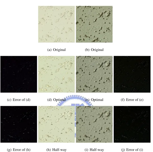
Figure 4.5: Reconstructed results comparison of our optimal reparameterization and half-way reparameterization. (a)(b) are textures of ceiling data from Bonn BTF database. (d)(e) are reconstructed results using our optimal reparameterization. (h)(i) are reconstructed results using half-way reparameterization. (c)(f)(g)(j) are error images of (d)(e)(h)(i) compare to (a)(b)(a)(b) respectively. Twenty multivariate SRBF kernels(J = 20) and three multivariate modes(K = 3) are used in (d)(e)(h)(i). The RMS error of (d)(e)(h)(i) are 0.029616, 0.040331, 0.032102, 0.042219 respectively.
4.3 Half-way Reparameterization vs. Optimal Reparameterization 22
(a) Original (b) Original
(c) Error of (d) (d) Optimal (e) Optimal (f) Error of (e)
(g) Error of (h) (h) Half-way (i) Half-way (j) Error of (i)
Figure 4.6: Reconstructed results comparison of our optimal reparameterization and half-way reparameterization. (a)(b) are textures of Impalla data from Bonn BTF database. (d)(e) are reconstructed results using our optimal reparameterization. (h)(i) are reconstructed results using half-way reparameterization. (c)(f)(g)(j) are error images of (d)(e)(h)(i) compare to (a)(b)(a)(b) respectively. Twenty multivariate SRBF kernels(J = 20) and three multivariate modes(K = 3) are used in (d)(e)(h)(i). The RMS error of (d)(e)(h)(i) are 0.060246, 0.064558, 0.063839, 0.081254 respectively.
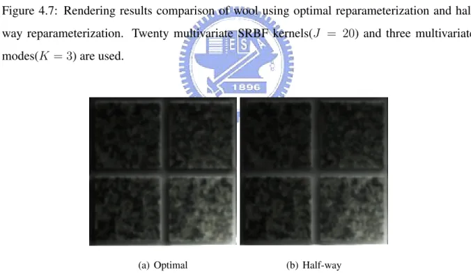
The rendering results comparison using optimal reparameterization and half way reparame-terization are shown in Figure 4.7 and Figure 4.8. Our optimal reparamereparame-terization keep the part
4.3 Half-way Reparameterization vs. Optimal Reparameterization 23 of self shadow more than half way reparameterization, and the details are preserved better using our optimal reparameterization.
(a) Optimal (b) Half-way
Figure 4.7: Rendering results comparison of wool using optimal reparameterization and half way reparameterization. Twenty multivariate SRBF kernels(J = 20) and three multivariate modes(K = 3) are used.
(a) Optimal (b) Half-way
Figure 4.8: Rendering results comparison of impalla using optimal reparameterization and half way reparameterization. Twenty multivariate SRBF kernels(J = 20) and three multivariate modes(K = 3) are used.
4.4 Smooth terms vs. No Smooth terms 24
4.4
Smooth terms vs. No Smooth terms
We set smooth terms to improve the quality and performance in rendering. Figure 4.10 shows some results of reconstruction of our BTF model with and without smooth terms. As we can see, details are better preserved than those without smooth terms, but if we do not set smooth terms, we can not use texture filter from hardware support to smooth coefficients $ of our BTF model in spatial domain, so we must reconstruct nearby pixels which is the bottleneck of performance and smooth it in color domain to render one pixel. Figure 4.9 shows the rendering results not using smooth terms and using smooth terms with texture filter from hardware support.
(a) No Smooth (b) Smooth
Figure 4.9: Rendering results comparison of corduroy without smooth terms and with smooth terms. Twenty multivariate SRBF kernels(J = 20) and three multivariate modes(K = 3) are used.
4.4 Smooth terms vs. No Smooth terms 25
(a) Original (b) Original (c) Original
(d) Smooth (e) Smooth (f) Smooth
(g) Without smooth (h) Without smooth (i) Without smooth
Figure 4.10: Reconstructed results comparison of our optimal parameter BTF model with smooth terms and without smooth terms. (a)(b)(c) are textures of corduroy data from Bonn BTF database. (d)(e)(f) are reconstructed results with smooth terms. (g)(h)(i) are reconstructed results without smooth terms. Twenty multivariate SRBF kernels (J = 20) and three multivari-ate modes (K = 3) are used in (c)(d)(e)(f)(g)(h)(i).
4.5 Time Consumption and Compression Ratio 26
4.5
Time Consumption and Compression Ratio
The modeling time of our optimal reparameterization is 1.5 times bigger than half-way reparameterization, and it takes less time to model BTF data which is more diffuse, such as wool and ceiling.
BTF Data Elapsed Time J K Reparameterization Min. Mipmap Level Corduroy 20 hour 25 min 6 sec 20 3 Half-way 1
Corduroy 29 hour 30 min 55 sec 20 3 Optimal 1 Wool 10 hour 6 min 24 sec 20 3 Half-way 1 Wool 16 hour 3 min 29. sec 20 3 Optimal 1 Ceiling 13 hour 12 min 5 sec 20 3 Half-way 0 Ceiling 20 hour 42 min 23 sec 20 3 Optimal 0 Impalla 12 hour 3 min 54 sec 20 3 Half-way 1 Impalla 17 hour 44 min 0.7 sec 20 3 Optimal 1
Table 4.1: Elapsed time of BTF modeling. J and K denote number of multivariate SRBF kernels and number of multivariate modes.
We store Coefficients $ of our BTF model $ in each level and each pixel with double, the data size is dependent on number of multivariate SRBF kernels and the number of levels. We find that resolution 128*128 is enough to keep great quality in rendering, so we use level 1 with resolution 128*128 as our minimum mipmap level. We use twenty multivariate SRBF kernels in most cases, so the compression ratio is about 1/6 compare to BTF data from Bonn.
4.6
Rendering Results
Figure 4.11 and Figure 4.12and Figure 4.13 Figure 4.14 are rendering results of wool and corduroy and ceiling BTF data. All these data are modeled using our optimal reparameteri-zation, wool and corduroy data are modeled with twenty BTF kernels and three multivariate
4.6 Rendering Results 27 BTF Data Data Size Lighting and Viewing Directions Resolution
Corduroy 327MB 81*81 256*256 Wool 346MB 81*81 256*256 Ceiling 2.05GB 81*81 800*800 Impalla 314MB 81*81 256*256
Table 4.2: Data size of data in BTF database Bonn. All textures are stored with JPEG format Data Size J K Min. Mipmap Level
52.1MB 20 3 1 26.1MB 10 3 1 204MB 20 3 0 104MB 10 3 0
Table 4.3: Data size of our BTF modeling. J and K denote number of multivariate SRBF kernels and number of multivariate modes.
modes, ceiling data are modeled with ten BTF kernels and three multivariate modes.
4.6 Rendering Results 28
Figure 4.12: Rendering result of corduroy with optimal reparameterization. (J=20,K=3)
4.6 Rendering Results 29
Figure 4.14: Rendering result of ceiling with optimal reparameterization. (J=10,K=3) The FPS of our BTF rendering is shown in Table 4.4. Evaluation time for each pixel fol-lows the number of multivariate SRBF kernels direct proportion relation, so the FPS using 20 multivariate SRBF kernels is about half of using 10 multivariate SRBF kernels.
Model triangle FPS J K Plane 800 50.23 10 3 Plane 800 26.10 20 3 Bunny 69630 18.77 10 3 Bunny 69630 9.42 20 3 cloth 59168 11.63 10 3 cloth 59168 6.15 20 3
Table 4.4: FPS of rendering. J and K denote number of multivariate SRBF kernels and number of multivariate modes.
C H A P T E R
5
Conclusion and Future Work
In this thesis, we use a data-driven parametric representation in viewing and lighting space to model the BTF data. Unlike fixed reparameterization, we can define reparameterization function and optimize their parameters to get the optimal reparameterization function. This optimal reparameterization can make BTF modeling more accurately.
To use spatial coherence efficiently, we construct mipmaps of BTF data and use mipmap hierarchy in our optimization process. We can speed up BTF modeling and keep the properties of mipmap which improves the performance and quality in rendering.
EM algorithm are used to speed up the heave work of optimization. We use EM algorithm to find a proper initial guess, so our optimization process works much faster and still remain great quality of results.
Our experiments has shown the improvement of our multivariate SRBF kernel and our op-timal reparameterization method compared to univariate SRBF kernel and half-way reparame-terization. Our BTF model is efficient both in modeling and rendering, our BTF model use only about one sixths than original BTF data and we can render our BTF model in real time.
Currently, there are some artifacts caused by mipmap and smooth terms. Fitting using multi-resolution hierarchy can speed up our framework a lot, but we assume corresponding textels in
31 different mipmap levels are similar. When the corresponding textels are totally different, it will induce large error, so how to solve this problem is the most important task in the future.
We smooth our BTF model in spatial dimension by adding difference value of nearby(5*5 square) into objective function. When the data differs a lot in this square, our smooth terms will cause bad influence, it increase error ratio in represent result. In the future, robust error matrix will be applied into our method to fix this problem.
Bibliography
[1] M. Alex, O. Vasilescu, and D. Terzopoulos. Tensortextures: Multilinear image-based rendering. ACM Transactions on Graphics, pages 336–342, 2004.
[2] W. chun Ma, S. hsiang Chao1, Y. ting Tseng, Y. yu Chuang, C. fa Chang, B. yu Chen, and M. Ouhyoung. Level-of-detail representation of bidirectional texture functions for real-time rendering. In Proceedings of I3D 2005, pages 187–194, 2005.
[3] O. G. Cula and K. J. Dana. Compact representation of bidirectional texture functions. In Proceedings of CVPR 2001, pages 1041–1047, 2001.
[4] K. J. Dana, B. V. Ginneken, S. K. Nayar, and J. J. Koenderink. Reflectance and texture of real-world surfaces. In Proceedings of ACM SIGGRAPH 1999, volume 18, pages 1–34, 1999.
[5] W. R. Davis. Cornelius Lanczos Collected Published Papers With Commentaries. North Carolina State University, 1999.
[6] D. B. Goldman, B. Curless, A. Hertzmann, and S. M. Seitz. Shape and spatially-varying brdfs from photometric stereo. In Proceedings of ICCV 2005, pages 341–348, 2005. [7] J. Kautz and M. D. Mccool. Interactive rendering with arbitrary brdfs using separable
approximations. In Proceedings of EGWR 1999, pages 247–260, 1999.
Bibliography 33 [8] M. L. Koudelka, S. Magda, P. N. Belhumeur, and D. J. Kriegman. Acquisition, compres-sion, and synthesis of bidirectional texture functions. In Proceedings of Texture 2003, pages 59–64, 2003.
[9] E. P. F. Lafortune, S.-C. Foo, K. E. Torrance, and D. P. Greenberg. Non-linear approxima-tion of reflectance funcapproxima-tions. In Proceedings of ACM SIGGRAPH 1997, pages 117–126, 1997.
[10] D. Lathauwer, B. D. Moor, and J. Vandewalle. On the best rank-1 and rank-(r1,r2,. . .,rn) approximation of higher-order tensors. SIAM J Matrix Anal Appl, 21:1324–1342, 2000. [11] J. Lawrence, A. Ben-artzi, C. Decoro, W. Matusik, H. Pfister, R. Ramamoorthi, and
S. Rusinkiewicz. Inverse shade trees for non-parametric material representation and edit-ing. ACM Transactions on Graphics, 25:735–745, 2006.
[12] S. Lefebvre and H. Hoppe. Appearance-space texture synthesis. In Proceedings of ACM SIGGRAPH 2006, pages 541–548, 2006.
[13] T. Leung and J. Malik. Representing and recognizing the visual appearance of materials using three-dimensional textons. Proceedings of Texture 2003, 43(1):29–44, 2001. [14] M. D. McCool, J. Ang, and A. Ahmad. Homomorphic factorization of brdfs for
high-performance rendering. In Proceedings of ACM SIGGRAPH 2001, pages 171–178, 2001. [15] F. J. Narcowich and J. D. Ward. Nonstationary wavelets on the m-sphere for scattered
data. Applied and Computational Harmonic Analysis, 3(4):324–336, 1996.
[16] R. Ramamoorthi and P. Hanrahan. Frequency space environment map rendering. In Pro-ceedings of ACM SIGGRAPH 2002, pages 517–526, 2002.
[17] S. M. Rusinkiewicz. A new change of variables for efficient brdf representation. In Euro-graphics Workshop on Rendering, pages 11–22, 1998.
Bibliography 34 [18] M. Sattler, R. Sarlette, and R. Klein. Efficient and realistic visualization of cloth. In
Proceedings of Eurographics Symposium on Rendering, pages 167–178, 2003.
[19] Y. ting Tsai and Z. chung Shih. All-frequency precomputed radiance transfer using spher-ical radial basis functions and clustered tensor approximation. ACM Transactions on Graphics, 25:967–976, 2006.
[20] H. Wang, Q. Wu, L. Shi, Y. Yu, and N. Ahuja. Out-of-core tensor approximation of multi-dimensional matrices of visual data. In Proceedings of ACM SIGGRAPH 2005, pages 527–535, 2005.
[21] T. Zickler, S. Enrique, R. Ramamoorthi, and P. Belhumeur. Reflectance sharing: Image-based rendering from a sparse set of images. In Proceedings of Eurographics Symposium on Rendering, pages 253–264, 2005.