Optimal Ultrasmall Block-Codes for Binary
Discrete Memoryless Channels
Po-Ning Chen, Senior Member, IEEE, Hsuan-Yin Lin, Student Member, IEEE, and
Stefan M. Moser, Senior Member, IEEE
Abstract—Optimal block-codes (in the sense of minimum av-erage error probability, using maximum likelihood decoding) with a small number of codewords are investigated for the binary asymmetric channel (BAC), including the two special cases of the binary symmetric channel (BSC) and the Z-channel (ZC), both with arbitrary cross-over probabilities. For the ZC, the optimal code structure for an arbitrary finite blocklength is derived in the cases of two, three, and four codewords and conjectured in the case of five codewords. For the BSC, the optimal code structure for an arbitrary finite blocklength is derived in the cases of two and three codewords and conjectured in the case of four codewords. For a general BAC, the best codebooks under the assumption of a threshold decoder are derived for the case of two codewords. The derivation of these optimal codes relies on a new approach of constructing and analyzing the codebook matrix not rowwise (codewords), but columnwise. This new tool leads to an elegant definition of interesting code families that is recursive in the block-length and admits their exact analysis of error performance. This allows for a comparison of the average error probability between all possible codebooks.
Index Terms—Binary asymmetric channel (BAC), binary sym-metric channel (BSC), finite blocklength, flip codes, maximum like-lihood (ML) decoder, minimum average error probability, optimal codes, weak flip codes, Z-channel (ZC).
I. INTRODUCTION
S
HANNON proved in his ground-breaking work [1] that it is possible to find an information transmission scheme that can transmit messages at arbitrarily small error probability as long as the transmission rate in bits per channel use is below the so-called capacity of the channel. However, he did not provide a way on how to find such schemes, but used a proof technique based on random coding that ensures the codes’ existence. In particular, he did not tell us much about the design of codes apart from the fact that good codes may need to have a large blocklength.For many practical applications, exactly this latter constraint is rather unfortunate as we often cannot tolerate too much delay Manuscript received March 20, 2012; accepted December 22, 2012. Date of publication August 07, 2013; date of current version October 16, 2013. This work was supported by the National Science Council under Grants NSC 97–2221–E–009–003–MY3 and NSC 100–2221–E–009–068–MY3. Parts of this paper were presented at the 2011 IEEE Information Theory Workshop.
The authors are with the Department of Electrical and Computer Engi-neering, National Chiao Tung University, Hsinchu 30010, Taiwan (e-mail: [email protected]; [email protected]; [email protected]).
Communicated by I. Kontoyiannis, Associate Editor At Large.
Color versions of one or more of the figures in this paper are available online at http://ieeexplore.ieee.org.
Digital Object Identifier 10.1109/TIT.2013.2276893
(e.g., in interhuman communication, in time-critical control, and communication, etc.). Moreover, the system complexity usually grows exponentially in the blocklength. In consequence, having large blocklength might not be an option, but we have to restrict the codewords to some reasonable size. The question now arises what can theoretically be said about the performance of commu-nication systems with such restricted block size.
The last years have seen a renewed interest in the theoret-ical understanding of finite-length coding [2]–[5]. There are sev-eral possible ways of approaching the problem of finite-length codes. In [2], the authors fix an acceptable error probability and a finite blocklength and then find bounds on the maximal achiev-able transmission rate. This parallels the method of Shannon who set the acceptable error probability to zero, but allowed infinite blocklength, and then found the maximum achievable transmission rate (the capacity). A typical example in [2] shows that for a blocklength of 1800 channel uses and for an error probability of , one can achieve a rate of approximately 80 percent of the capacity of a binary symmetric channel of ca-pacity 0.5 bits. For more details about the work in [2], we refer to Section VI-C.
In a different approach, one fixes the transmission rate and studies how the error probability depends on the blocklength (i.e., one basically studies error exponents, but for relatively small [6]). For example, [5] introduces new random coding bounds that enable a simple numerical evaluation of the error probability for finite blocklengths.
All these results have in common that they are related to Shannon’s ideas in the sense that they try to make fundamental statements about what is possible and what not. The exact manner how these systems have to be built is ignored on purpose.
Our approach in this paper is different. Based on the insight that for very short blocklength, one has no big hope of trans-mitting much information with acceptable error probability, we concentrate on codes with a small fixed number of codewords: so-called ultrasmall block-codes. By this reduction of the trans-mission rates, our results are directly applicable even for very short blocklengths. In contrast to [2] that provides bounds on the best possible theoretical performance, we try to find a best possible design that minimizes the average error probability. Hence, we put a big emphasis on finding insights in how to ac-tually build an optimal system. In this respect, this paper could rather be compared to [7]. There the authors try to describe the empirical distribution of good codes (i.e., of codes that approach capacity with vanishing error probability) and show that for a large enough blocklength, the empirical distribution of certain 0018-9448 © 2013 IEEE
good codes converges in the sense of divergence to a set of input distributions that maximize the input–output mutual informa-tion. Note, however, that [7] again focuses on the asymptotic regime, while our focus lies on finite blocklength, and not ca-pacity-achieving codes.
There are interesting applications for ultrasmall block-codes. For example, in the situation of establishing an initial connec-tion in a wireless link, the amount of informaconnec-tion that needs to be transmitted during the setup of the link is very limited, usually only a couple of bits, but these bits need to be transmitted in very short time (e.g., blocklength in the range of to ) with the highest possible reliability [8]. Another important ap-plication for ultrasmall block-codes is in the area of quality of service (QoS). In many delay-sensitive wireless systems like, e.g., voice over IP (VoIP) and wireless interactive and streaming video applications, it is essential to comply with certain limita-tions on queuing delays or buffer violation probabilities [3], [4]. A further area where the performance of short codes is relevant is proposed in [9]: effective rateless short codes can be used to transmit some limited feedback about the channel state informa-tion in a wireless link or in some other latency-constrained ap-plication. Hence, it is of significant interest to conduct an anal-ysis of (and to provide predictions for) the performance levels of practical finite-blocklength systems. Note that while the mo-tivation of this work focuses on rather smaller values of , our results nevertheless hold for arbitrary finite .
The study of ultrasmall block-codes is interesting not only be-cause of the above-mentioned direct applications, but bebe-cause their analytic description is a first step to a better fundamental understanding of optimal nonlinear coding schemes (with ML decoding) and of their performance based on the exact error probability rather than on an upper bound on the achievable error probability derived from the union bound or the mutual information density bound and its statistics [10], [11].
To simplify our analysis, we have restricted ourselves for the moment to binary discrete memoryless channels, that we call in their general form binary asymmetric channels (BAC). The two most important special cases of the BAC, the binary symmetric
channel (BSC) and the Z-channel (ZC), are then investigated
more in detail.
Our main contributions are as follows:
1) We provide first fundamental insights into the performance analysis of optimal nonlinear code design for the BAC. Note that there exists a vast literature about linear codes, their properties, and good linear design (e.g., [12]). Some Hamming-distance related topics of nonlinear codes are addressed in [13].1
2) We provide new insights in the optimal code construction for the BAC for an arbitrary finite blocklength and for
codewords.
3) We provide optimal code constructions for the ZC for an arbitrary finite blocklength and for , 3 and 4 code-words. For the BSC, we provide optimal code construc-tions for an arbitrary finite blocklength and for
1Note that some of the code designs proposed in this paper actually have
interesting “linear-like” properties and can be considered as generalizations of linear codes with codewords to codes with a general number of codewords
. For more details see [14].
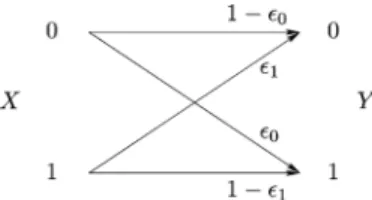
Fig. 1. Binary asymmetric channel (or BAC).
and 3 codewords and locally optimal code constructions
for codewords.
4) We propose a new approach to the design and analysis of block-codes: instead of focusing on the codewords (i.e., the rows in the codebook matrix), we look at the codebook matrix in a columnwise manner.
The remainder of this paper is structured as follows: we end this introduction with some comments about our notation and will then introduce our channel models in Section II. After some more preliminaries in Section III, Section IV contains a very short example showing that the analysis of even such simple channel models is nontrivial and often nonintuitive. Section V then presents new code definitions that will be used for our main results. In Section VI, we review some important previous work. Sections VII–IX then contain our main results. In Section VII, we analyze the BAC for two codewords, Section VIII takes a closer look at the ZC, and in Section IX we investigate the BSC. Many of the lengthy proofs have been moved to the appendix. We conclude in Section X.
As is common in coding theory, vectors (denoted by bold face Roman letters, e.g., ) are row-vectors. However, for simplicity of notation and to avoid a large number of transpose-signs, we slightly misuse this notational convention for one special case: any vector is a column-vector. It should be always clear from the context because these vectors are used to build codebook matrices and are therefore also conceptually quite different from the transmitted codeword or the received sequence . Other-wise our used notation follows the main stream. We use capital letters for random quantities, e.g., , and small letters for real-izations, e.g., ; sets are denoted by a calligraphic font, e.g., ; and constants are depicted by Greek letters, small Romans or a special font, e.g., .
II. CHANNELMODEL ANDSYSTEMDESCRIPTION We consider a discrete memoryless channel (DMC) with both a binary input and a binary output alphabet. The most general such binary DMC is the so-called binary asymmetric channel (BAC) and is specified by two parameters: denotes the prob-ability that a 0 is flipped into a 1, and denotes the probability that a 1 is flipped into a 0, see Fig. 1.
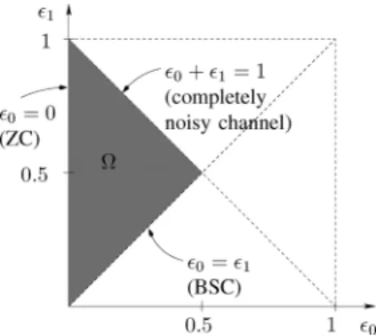
For symmetry reasons and without loss of generality, we can restrict the values of these parameters as follows:
(1) (2) (3) Note that in the case when , we simply flip all zeros to ones and vice versa to get an equivalent channel with .
Fig. 2. Region of possible choices of the channel parameters and of a BAC. The shaded area corresponds to the interesting area according to (1)–(3).
Fig. 3. Binary symmetric channel.
Fig. 4. Z-channel.
For the case when , we flip the output , i.e., change all output zeros to ones and ones to zeros, to get an equivalent channel with . Note that (2) can be simplified to and is actually implied by (1) and (3). And for the case
when , we flip the input to get an equivalent
channel that satisfies .
We have depicted the region of possible choices of the param-eters and in Fig. 2. The region of interest given by (1)–(3) is denoted by .
Note that the boundaries of correspond to three special cases: the binary symmetric channel (BSC) (see Fig. 3) has equal cross-over probabilities . According to (2), we can assume without loss of generality that .
The Z-channel (ZC) (see Fig. 4) will never distort an input 0, i.e., . An input 1 is flipped to 0 with probability .
Finally, the case corresponds to a completely noisy channel of zero capacity: given , the events and are equally likely, i.e., and are statistically independent.
The following three definitions are commonly used.
Definition 1: An coding scheme for a channel
con-sists of a codebook with codewords of length
( ), an encoder that maps every message into
its corresponding codeword , and a decoder that makes a
de-coding decision for every received -vector
.
A codebook is called linear if it can be seen as a subspace of the -dimensional vector space over the channel input alphabet.2
The performance of a coding scheme is described by its av-erage probability of making a decoding error.
Definition 2: Given that message has been sent, let be the probability of a decoding error of a code:
(4) (5) where is the indicator function whose value is 1 if the state-ment is correct and 0 otherwise. The average error probability
of a code is defined as
(6) Sometimes it will be more convenient to focus on the probability of not making any error, denoted success probability :
(7) and on the corresponding average success probability3
.
We will always assume that the possible messages are equally likely and that the decoder is a maximum likelihood (ML) decoder:
(8)
Note that for equally likely messages, an ML decoder is equiva-lent to a maximum a posteriori (MAP) decoder and is therefore optimal.
Definition 3: For a given coding scheme, we define the decoding region as the set of -vectors that are decoded to the message :
(9) Moreover, we also make the following definitions.
Definition 4: By we denote the number of
po-sitions , where and . For , the joint
composition of two codewords and is de-fined as
(10)
Note that and
denote the commonly used Hamming distance and Hamming weight, respectively.
2Being a subspace, linear codes usually are represented by a generator matrix,
which is basically a basis of the subspace. As we are not interested in linear codes in particular, but in both linear and nonlinear codes, we will not use this in this paper.
The following remark deals with the way how codebooks can be described. It is not standard, but turns out to be very important and is actually a clue to our derivations.
Remark 5: It is usual to write the codebook as an matrix with its rows corresponding to the codewords
..
. (11)
However, it turns out to be much more convenient and powerful to consider the codebook columnwise instead of rowwise. So, instead of specifying the codewords of a codebook, we actually specify its (length- ) column-vectors .
Remark 6: Since we assume equally likely messages, any
permutation of rows only changes the assignment of codewords to messages and has no impact on the performance. We consider two codes with permuted rows as being equal, i.e., a code is ac-tually a set of codewords, where the ordering of the codewords is irrelevant.
Furthermore, since we are only considering memoryless channels, any permutation of the columns of will lead to another codebook that is equivalent to the first in the sense that it has the exact same error probability. We say that such two codes are equivalent. We would like to emphasize that two codebooks being equivalent is not the same as two codebooks being equal. However, as we are mainly interested in the performance of a codebook, we usually treat two equivalent codes as being the same. In particular, when we speak of a unique code design, we do not exclude the always possible permutations of columns.
In spite of this, for the sake of clarity of our derivations, we usually will define a certain fixed order of the codewords/code-book column vectors.
III. PRELIMINARIES
A. Error Probability of the BAC
The conditional probability of the received vector given the sent codeword of the BAC can be written as
(12) where we use to denote the product distribution
(13)
Considering that
(14)
the average error probability of a coding scheme over a BAC can now be written as
(15)
(16) where is the ML decision (8) for the observation .
B. Error (and Success) Probability of the BSC
In the special case of a BSC, (16) simplifies to
(17)
The success probability is accordingly4
(18)
C. Error (and Success) Probability of the ZC
In the special case of a ZC, the average success probability can be expressed as follows:
(19)
(20) The error probability formula is accordingly
(21)
4Note that the second summation contains only one value and could be
D. Pairwise Hamming Distance
The minimum Hamming distance is a well-known and often used quality criterion of a codebook, see, e.g., [12], [13]. In [13, Ch. 2], the maximum minimum Hamming distance for a given code is discussed including important results like the Plotkin bound and Levenshtein’s theorem. (For more de-tails about upper and lower bounds to the average error proba-bility, see also Section VI.) Unfortunately, a design based on the minimum Hamming distance can fail even for linear codes and even for a very symmetric channel like the BSC, whose error probability performance is completely specified by the Ham-ming distances between codewords and received vectors (see also Section IX-C).
We therefore define a slightly more general and more con-cise description of a codebook: the pairwise Hamming distance
vector.
Definition 7: Given a codebook with codewords , , we define the pairwise Hamming distance vector
of length as follows:
(22)
The minimum Hamming distance is then defined
as the minimum component of the pairwise Hamming distance
vector .
IV. ANEXAMPLE
To show that the search for an optimal (possibly nonlinear) code is neither trivial nor intuitive even in the symmetric BSC case, we would like to start with a simple example before we summarize our main results.
Assume a BSC with cross-over probability , ,
and a blocklength . Then consider the following codes:5
(23) We observe that while both codes are linear, the first code has a minimum Hamming distance 1, and the second has a min-imum Hamming distance 2. It is quite common to believe that shows a better performance. This intuition is based on Gallager’s famous performance bound [6, Ex. 5.19]:
(24) However, the exact average error probability as given in
(17) actually can be evaluated as and
5We will see in Section V that both codes are weak flip codes. In this example,
and according to Definition 11 given later.
. Hence, even though the minimum Ham-ming distance of the first codebook is smaller, its overall performance is superior to the second codebook!
Our goal is to find the structure of an optimal code that satisfies
(25)
for any code .
V. FLIPCODES ANDWEAKFLIPCODES
We next introduce some special codebooks that will prove instrumental in developing the optimal codes.
Definition 8: The flip code of type , , for is a code with codewords defined by the following codebook matrix:
(26) Defining the column vectors
(27) we see that a flip code of type is given by a codebook matrix consisting of first columns and then columns .
We again remind the reader that due to the memorylessness of the BAC, other codes with the same columns as , but in different order are equivalent to . Moreover, we would like to point out that while the flip code of type 0 corresponds to a repetition code, the general flip code of type with is neither a repetition code nor is it even linear.
The columns given in the set (27) are called candidate
columns. They are flipped versions of each other, therefore also
the name of the code.
The definition of a flip code with one codeword being the flipped version of the other cannot be easily extended to a sit-uation with more than two codewords. Hence, for , we need a new approach. Motivated by (27) and noting that these candidate columns have an equal number of zeros and ones, we give the following definition.
Definition 9: For an , a length- candidate column is called a weak flip column if its first component is 0 and its
Hamming weight equals to or .
Accordingly, a weak flip column contains an equal or at least almost equal number of zeros and ones. Note, however, that only
in (27) is a weak flip column.
Based on these weak flip columns, we define the family of
weak flip codes.
Definition 10: A weak flip code is defined by a codebook
matrix that is constructed solely by weak flip columns. Note that for , only the flip code of type 0 also is a weak flip code, all other flip codes are not weak flip codes, i.e., the definition of weak flip codes is only useful for .
For or , we define the weak flip codes more
specifically as follows.
Definition 11: A weak flip code of type , , with or codewords is defined by a codebook matrix
consisting of first columns , then columns , and finally columns , where
(28) or
(29) respectively. We often describe the weak flip code of type
by its code parameters
(30) where can be computed from the blocklength and the type
as . Moreover, we use
(31) to denote the decoding region of the th codeword of .
Note that, as already discussed in Remark 6, the order of these columns does not matter with regard to the performance of the code. However, in order to make sure that the code is well de-fined, we require here the order of the candidate columns to be exactly as given (i.e., all columns together, then all in the middle, and all on the right of the codebook matrix). Thereby, we also clearly and uniquely specify the codewords
.
An interesting subfamily of weak flip codes is defined as follows.
Definition 12: A fair weak flip code of type ,
with or codewords satisfies that
(32) Note that the fair weak flip code is only defined provided that the blocklength satisfies . In order to be able to pro-vide convenient comparisons for every blocklength , we de-fine a generalized fair weak flip code for every , , where
(33) If , the generalized fair weak flip code actually is a fair weak flip code.
The following lemma follows straightforwardly from the re-spective definitions. We therefore omit its proof.
Lemma 13: The pairwise Hamming distance vector of the
weak flip code for or is given as follows:
(34) (35) VI. PREVIOUSWORK
A. SGB Bounds on the Average Error Probability
In [15], Shannon, Gallager, and Berlekamp derive upper and lower bounds on the average error probability of a given code used on a DMC. We next quickly review their results.
Definition 14: For , we define
(36)
Then, the discrepancy between and is
defined as
(37)
with given in Definition 4.
Note that the discrepancy is a generalization of the Ham-ming distance, however, it depends strongly on the conditional channel law (i.e., in the case of a BAC, on the cross-over proba-bilities). We use a superscript “(DMC)” to indicate the channel which the discrepancy refers to.
Definition 15: The minimum discrepancy
for a codebook is the minimum value of over
all pairs of codewords. The maximum minimum discrepancy is
the maximum value of over all possible
codebooks: .
Theorem 16 (SGB Bounds on Average Error Probability [15]): For an arbitrary DMC, the average error probability
of a given code with codewords and
blocklength is upper- and lower-bounded as follows:
(38) where denotes the smallest nonzero transition probability of the channel.
Note that these bounds are specific to a given code design (via ). Therefore, the upper bound is a generally valid upper bound on the optimal performance, while the lower bound only holds in general if we apply it to the optimal code or to a suboptimal code that achieves the optimal .
The bounds (38) are tight enough to derive the error exponent of the DMC (for a fixed number of codewords).
Theorem 17 ([15]): The error exponent of a DMC for a fixed
number of codewords
(39) is given as
(40) Unfortunately, in general the evaluation of the error exponent is very difficult. For some cases, however, it can be done. For
example, for , we have
(41) Also for the class of so-called pairwise reversible channels, the calculation of the error exponent turns out to be uncomplicated.
Definition 18: A pairwise reversible channel is a DMC that
has for any inputs .
Note that it is easy to compute the pairwise discrepancy of a linear code on a pairwise reversible channel, so linear codes are quite suitable for computing (38).
Theorem 19 ([15]): For pairwise reversible channels with
,
(42) where denotes the number of times the channel input letter occurs in a column. Moreover, is achieved by fair weak flip codes.6
We would like to emphasize that while Shannon et al. proved that fair weak flip codes achieve the error exponent, they did not investigate the error performance of fair weak flip codes for finite . As we will show later, fair weak flip codes might be strictly suboptimal for finite (see also [16]).
B. Gallager Bound
Another famous bound is by Gallager [6].
Theorem 20 ([6]): For an arbitrary DMC, there exists a code
with such that
(43) where is the Gallager exponent and is given by
(44) with
(45)
C. PPV Bounds for the BSC
In [2], Polyanskiy, Poor, and Verdú present upper and lower bounds on the optimal average error probability for finite blocklength for the BSC. The upper bound is based on random
coding. It is the exact random coding error expression for the
BSC by using an alternative way compared to [17].
Theorem 21 (PPV Upper Bound [17, Theorem 2],[2, Theorem 32]): If the codebook is created at random based on a uniform distribution, the expected average error probability (av-eraged over all codewords and all codebooks) satisfies
(46)
6While throughout we only consider binary inputs and or ,
the definitions of our fair weak flip codes can be extended to nonbinary inputs and larger . Also, these extended fair weak flip codes will achieve the corre-sponding error exponents. Note that Shannon et al. did not actually name their exponent-achieving codes.
Note that there must exist a codebook whose average error probability achieves (46), so Theorem 21 provides a general achievable upper bound on the error probability, although we do not know the concrete code structure.
Polyanskiy et al. also provide a new general converse for the average error probability: the so-called metaconverse, which is based on binary hypothesis testing. For a BSC, the meta-converse lower bound happens to be equivalent to Gallager’s sphere-packing bound.
Theorem 22 (PPV Lower Bound [6, p. 163, Eq. (5.8.19)],[2, Theorem 35]): Any codebook satisfies
(47)
where for and for
(48) and where the positive integer and coefficients are chosen such that
(49)
(50) VII. ANALYSIS OF THEBAC
We start with results that hold for the general BAC. In this section, we will restrict ourselves to two codewords . Note that in this analysis we do not focus on performance bounds, but we put a special emphasis on the optimal code design.
A. Optimal Codes
Theorem 23: Consider a BAC and a blocklength . Then,
irrespective of the channel parameters and , there exists a choice of , , such that the flip code of type , is optimal in the sense that it minimizes the average error probability.
Proof: Consider an arbitrary code with codewords and a blocklength , and assume that this code is not a flip code, but it has a number of positions where both codewords have the same symbol. An optimal decoder will ignore these positions completely. Hence, the performance of this code will be identical to a flip code of length . Now, change this code in the positions with identical symbol such that the code becomes a flip code of length . If we use a suboptimal decoder that ignores these positions we still keep the same performance. However, an ML decoder can potentially improve the perfor-mance, i.e., we have
(51) (52)
An alternative proof is shown in Appendix A-B. While this proof is more elaborate, it turns out to be useful for the deriva-tion of Theorem 25.
This result is intuitively very pleasing because it seems to be a rather bad choice to have both codewords having the same symbol in a particular position, e.g., in the same position . However, note that the theorem does not exclude the possibility that another code might exist that also is optimal and that does have an identical symbol in both codewords at a given position.
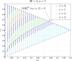
We would like to point out that the exact choice of is not obvious and depends strongly on , , and . As an example, the optimal choices of are shown in Fig. 5 for as a function of and . We see that depending on the channel parameters, the optimal value of changes. Note that for a com-pletely noisy channel ( ), the choice of is irrelevant since the probability of error is for any code. Moreover, in Theorem 29 it will be shown that the flip code of type 0 is op-timal on the ZC; and in Theorem 36 it will be shown that the flip codes are optimal on the BSC for any choice of . We defer the exact treatment of the ZC and the BSC to Sections VIII and IX, respectively.
B. Optimal Decision Rule for Flip Codes
Having only two codewords, the ML decision rule can be expressed using the log-likelihood ratio (LLR). For the flip code of type , , the LLR is given as
(53)
(54) (55) (56) where we have defined
(57) to be the Hamming distance of the received sequence to the first codeword.
Hence, we now express the ML decision rule for the flip code of type as
(58) Recall that and are parameters describing the channel (BAC), and describe the codebook (flip code ), and describes the received vector (with respect to the first codeword). As an example, Fig. 6 depicts the log-likelihood
Fig. 5. Optimal codebooks on a BAC: the optimal choice of the parameter for different values of and for a fixed blocklength .
Fig. 6. Log-likelihood ratio for (i.e., ) as a function of for different values of . The solid blue lines corre-spond to , the dashed red lines to . Observe that for and (i.e., the region between the two vertical purple lines), the threshold for the optimal ML decision rule is , see Theorem 24.
ratio as a function of (with )
for the flip code in the cases of and . We see
that for some integer , is always larger than
0 for and smaller than 0 for .
This seems to point toward a simplification of (58): instead of computing the log-likelihood ratio, we only need to consider . This indeed is the case. From Properties (2) and (3) of Propo-sition 40 in Appendix A-A, it follows directly that the ML de-cision rule for a flip code is a threshold rule.
Theorem 24 (Threshold Rule): For every flip code and
every BAC , there exists a threshold ,
, such that the ML decision rule can be stated as if
if . (59)
The threshold depends on . The region of channel pa-rameters with identical threshold (for given and ) is then defined as follows:
Fig. 7. Error probabilities of all possible flip codes as a function of the channel parameter , for a fixed blocklength , , and a fixed decision rule . For any , the best code is the one with the smallest error probability value.
C. Best Codes for a Fixed Decision Rule
Our original goal was to find the optimal code for a given channel . We have shown that this is equivalent to finding an optimal . Unfortunately, this search is difficult because the borders between the regions of different optimal (see, e.g., Fig. 5) are defined by the combined influences of two different forces: when varying , either the optimal code changes, but the optimal threshold remains the same, or the optimal choice of changes, too. Hence, a joint optimization of
and is necessary.
We now simplify the problem by fixing the decision rule (i.e., the threshold ) and then search for the best code for the given threshold and the given channel . This turns out to be easier, but unless we happen to have chosen the optimal for the given BAC , this will result in a suboptimal solution.
We start with the following interesting result that links the roots of the LLR-function with choices of parameters for which two different codes have identical error probability. This will then allow us to find the boundaries where the best codes under a fixed decision rule change from to (see also Fig. 8 below).
Theorem 25: Fix a blocklength , a code parameter
, and a decision rule threshold . Then, the roots of (61) are identical to the roots of
(62) where denotes the error probability of code decoded under the decision threshold . Moreover, for a fixed
, there exists at most one such that (61) holds; and for a fixed , there exists at most one such that (61) holds. This means that if (61) has a solution, then this solution is unique for a fixed or .
Proof: See Appendix A-C.
Using Theorem 25 and Proposition 40, we can now state con-ditions on such that is best under a fixed decision rule .
Fig. 8. Best codebooks on a BAC for a fixed decision rule: for all possible this plot shows the best choice of the code parameter . The blocklength is and the decision rule is .
Corollary 26: Fix a blocklength and a decision rule . Then,
the flip code of type , is uniquely best for a fixed decision rule if and only if belongs to
(63) If the region is empty, then is not best for any channel.
Proof: From (140) in the Proof of Theorem 25 in
Appendix A-C and from assumption (1) it follows that
(64)
As we know from Proposition 40 that is
increasing in , this means that if both (64) and
(65) are satisfied, the code is best for the given channel , for the given blocklength , and for the fixed decision rule .
We illustrate Corollary 26 by an example. We fix ,
, , and let increase from 0 to ,
see Fig. 7. Starting with , we check that
(66)
for all , i.e., . Next, we check
:
(67) for small , i.e., the code is best for those . When
in-creasing as soon as , there is a
change and becomes best. Further increasing while keeping then finally reveals the last change that happens
at the root of . So there are three best codes
for :
Fig. 9. Globally optimal codebooks on a BAC for a blocklength (iden-tical to Fig. 5). The shown boundary between and is identical to the corresponding boundary given in Fig. 8, where a fixed decision rule has been assumed.
2) is best in
.
3) is best in .
In Fig. 7, the error probabilities of the various flip codes are shown as a function of . The best choices of for all values of
for and are shown in Fig. 8.
Corollary 26 shows that for a fixed decision rule , the choice of the best code parameter depending on the given parameters , , and is much easier than the choice of the jointly optimal and for a globally optimal code. In particular, we have the following regular structure.
Corollary 27: Fix a blocklength and a decision rule , and consider a BAC. If we increase or decrease , then the best value of is nonincreasing.
More sloppily, we can say that when we are moving inside of (see Fig. 2) to the right or downward, the best will either remain the same or be reduced by 1. This is in stark contrast to the picture of the regions of optimal codes where the optimal changes in a seemingly random manner. For an illustration, compare the best codes for a fixed decision rule in Fig. 8 with the corresponding globally optimal regions of Fig. 5.
Even more importantly, Theorem 25 also allows us to locate the exact location of some of the boundaries between the dif-ferent areas of globally optimal codes (see Fig. 5).
Corollary 28: Consider the boundary between two areas of
globally optimal codes (as, e.g., shown in Fig. 5). If the op-timal decision rule on both sides of the boundary takes the same value and if the optimal code on the left is , while the optimal code on the right is , then this boundary is identical to a corresponding boundary in the situation with a fixed deci-sion rule . In particular, this boundary is given by the roots of
.
We again show the example of from Fig. 5: in Fig. 9, the same plot is shown including a boundary that is identical to a boundary given in Fig. 8.
We also would like to point out that the results for a given fixed decision rule simplify the search for a globally optimal code considerably. Such a search can be summarized by the following algorithm.
Step 0: Fix a channel and find the best under the fixed decision rule and its corresponding error
probability . Then, set .
Step 1: Find the best under a fixed decision rule and the corresponding error probability .
Step 2: Check whether . If yes, set
and .
Step 3: If , and return to Step 1.
Otherwise put out (describing the optimal code) and (giving the minimum error probability).
VIII. ANALYSIS OF THEZC
In this section, we investigate the special case of a ZC more in detail.
A. Optimal Codes With Two Codewords ( )
Theorem 29: For a ZC and for any , an optimal code-book with two codewords is the flip code of type 0,
. It has an error probability
(68)
Proof: Due to Theorem 23, we can restrict our search to
flip codes of some type , , i.e., is the flipped
version of .
For such a flip code, we observe that due to the peculiarity of the ZC that will never flip a zero to a one, an error can only occur when the received vector is the all-zero vector :
if
if . (69)
This error probability is minimized if one of the codewords is the all-one codeword; hence, is optimal.
Note the optimal code is linear. Moreover, from the proof it also follows that is the unique optimal code.
B. Optimal Codes With Three or Four Codewords ( )
Before we describe how we address the optimal codes with 3 or 4 codewords for a ZC, we first show that an optimal code must contain the all-zero vector as a codeword.
Theorem 30 (Sufficient Set of Candidate Columns for the ZC):
For a ZC, for any blocklength , and for an arbitrary number of codewords, an optimal codebook must contain the all-zero codeword .
Proof: See Appendix B-A.
Next we show that the weak flip codes of type are optimal codes with three or four codewords for a ZC.
Theorem 31: For a ZC and for any , an optimal
code-book with three codewords or four codewords is
the weak flip code of type , , with
(70) Moreover, the optimal code achieves the average error probability
if
if . (71)
Proof: See Appendix B-B.
Similarly to the case of , we see that for the optimal code given in Theorem 31 is linear. Also note that from the discussion in Appendix B-B it follows that for even , these linear codes are the unique optimal codes, while for odd there are other (also nonlinear) designs that achieve the same optimal performance.
For , the optimal codes are not unique. Indeed any
choice of and with is optimal.
It is remarkable that these optimal codes perform quite well even for a very short blocklength. As an example, consider four
codewords of blocklength that are used over
a ZC with . The optimal average error probability
is . If we increase the blocklength
to , we already achieve an average error probability . The asymptotic behavior of the op-timal error probability for going to infinity will be discussed in next section.
Next we will investigate the optimal code design from a new perspective: based on the fact that we consider a DMC, i.e., a channel that is memoryless and stationary, we would like to construct the codes recursively in the blocklength .
We start with the following lemma.
Lemma 32: Fix some arbitrary integers , , and . Consider a DMC and a code for this DMC with codewords and blocklength , and create a new code
by appending arbitrary column vectors to the codebook ma-trix of . Then, the average success probability of this new code cannot be smaller than the success probability of the orig-inal code:
(72)
Proof: For a given code , the average success prob-ability is given by
(73)
Now we consider the new codebook that is formed by appending columns to the original codebook matrix of . For convenience, we express the new codewords by
(74) (75)
and likewise the extended received vector by
(76) Assume that a length- received vector is in the th
de-coding region, . According to the ML decoding
rule, a corresponding new received vector will change to another decoding region if
(77)
Obviously, if no extended received vectors change its original decoding region from its length- counterpart, then
(78)
(79) where denotes the output alphabet. However, if some changes its original decoding region of blocklength , the new success probability will be
(80) (81) The proof of Lemma 32 is completed by noting that, from (77),
is always nonnegative.
Definition 33: The term in (81) is called total
probability increase for a step-size and describes the amount by which the average success probability of the code grows when column vectors are appended to its codebook matrix.
Lemma 34: For a ZC, for any , and for , consider the weak flip code of type with four codewords , , and append a column to the codebook matrix to create a new code of length . Then, the total probability increase is maximized if, among all possible columns,
we choose . If , or if is odd and , then
this choice is unique.
For , appending or to is equally
optimal.
We would like to point out that the codes can be seen as double-flip codes consisting of the combination of the (two-codeword) flip code of type 0 with the (two-(two-codeword) flip code
of type :
(82)
with and defined in (26).
From the recursive technique that we have used in the deriva-tion of Lemma 34 and that is based on the addideriva-tion of columns to the codebook matrix, it immediately follows that our optimal codes can be constructed recursively in . Concretely, we have the following corollary.
Corollary 35: The optimal codebooks defined in Theorem
31 for and can be constructed recursively in
the blocklength by adding a column that yields the maximum total probability increase. We start with an optimal codebook
for :
(83) Then, we recursively construct the optimal codebook for
by using and appending
if
if . (84)
Proof: We only need to show that the constructed codes
from (84) are equivalent to the optimal codes given in Theorem 31. The optimal code for and is trivial and given by (83). Next assume that for blocklength , is optimal. From Lemma 34, we know that the largest total probability in-crease is achieved when adding column . Now note that for
even with , adding the column to the code will result in a code that is equivalent to : we only need to exchange the roles of the second and third codeword and then re-order the columns. For odd with , adding
the column to the code results in .
Hence, we see that is still optimal. The claim now follows by induction in . The case with three codewords can be proved in a similar manner.
Note that we have actually proven that any codebook con-sisting of columns and columns arbitrarily chosen from or is optimal on a ZC (see the main discussion in Appendix B-B).
We conclude this section by a remark. While it is very intu-itive to construct the codes recursively, i.e., to start from an op-timal code for and then to add one column that maximizes the total probability increase, unfortunately, from a proof perspec-tive, such a recursive construction only guarantees local opti-mality: one still needs a proof (Theorem 31) that the achieved code of blocklength is globally optimum.
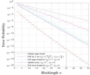
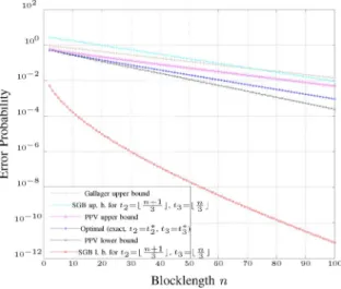
Fig. 10. Exact value of, and bounds on, the performance of an optimal code with codewords on the ZC with as a function of the block-length .
C. Error Exponents
Since the ZC is not pairwise reversible, the error exponents
for or codewords were previously unknown.
Using that for the optimal code we have if
if (85)
we can now compute the error exponents
(86)
Note that the minimum discrepancy for the
generalized fair weak flip code for every is if if
if .
(87)
D. Application to Known Bounds on the Error Probability for a Finite Blocklength
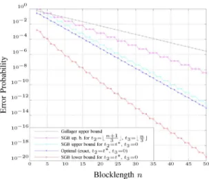
Since we now know the optimal code structure and its per-formance, it is interesting to compare it to the known bounds described in Section VI. Figs. 10 and 11 compare some SGB bounds and the Gallager bound with the exact performance of
the optimal code (for and codewords,
respec-tively). Besides the Gallager bound, we plot the SGB lower bound based on the optimal code structure (thereby making sure that this lower bound is valid generally), and we show two SGB upper bounds: one that is based on the optimal code design and one that is based on the fair weak flip code used by Shannon
et al.
We see that the SGB upper bound that is based on the optimal code is quite close to the exact performance, in particular, it exhibits the correct error exponent. The SGB upper bound that is based on the fair weak flip code, on the other hand, does not achieve the error exponent (which can be expected because the ZC is not pairwise reversible). Also the Gallager bound does not achieve the correct exponential behavior. The SGB lower bound is quite loose.
Fig. 11. Exact value of, and bounds on, the performance of an optimal code with codewords on the ZC with as a function of the block-length .
E. Conjectured Optimal Codes With Five Codewords ( )
The idea of designing an optimal code recursively promises to be a very powerful approach. Unfortunately, for larger values of , we might need a recursion from to with a step-size . In the following, we conjecture an optimal code construction for a ZC in the case of five codewords with a different recursive design for odd and even (i.e., with a
step-size ).
We define the following five weak flip column vectors:
(88)
We claim that an optimal code can be constructed recursively for even in the following way. We start with an optimal codebook
for :
(89) Then, we recursively construct the optimal codebook for
, even, by using and appending
if if if if if . (90)
For odd, we start with the length-9 code
(91) and recursively construct the optimal codebook for ,
odd, by using and appending
if if if if if . (92)
Note that the recursive structure in (90) and (92) is actually iden-tical apart from the ordering. Also note that when increasing the blocklength by 10, we add each of the five column vectors in (88) exactly twice. For , the optimal code structure goes through some transient states.
IX. ANALYSIS OF THEBSC
A. Optimal Codes With Two Codewords ( )
Theorem 36: For a BSC and for any , an optimal code-book with two codewords is the flip code of type for
any .
Proof: From Theorem 23, we already know that there must
exist a flip code that is optimal. Moreover, Theorem 23 also shows that the all-zero and the all-one column in a codebook matrix is strictly suboptimal. So, we only have two possible choices of candidate columns: and . By the sym-metry of a BSC, both columns will result in an identical perfor-mance. Therefore, every flip code has the same performance, i.e., all of them must be optimal.
B. Optimal Codes With Three or Four Codewords ( )
Unlike in the case of a ZC, for a BSC it is not easy to derive the exact average error probability expressed only by the candi-date column parameters . So instead we use a recursive code construction that guarantees largest total probability increase.
Theorem 37: For a BSC with arbitrary cross-over probability
, the optimal code with three codewords or
four codewords and with a blocklength is
(93) If we recursively construct a locally optimal codebook with
three codewords or four codewords and with
a blocklength by using and appending a new
column, the total probability increase is maximized by the fol-lowing choice of appended columns:
if if
if .
Proof: See Appendix C-A.
While Theorem 37 only guarantees local optimality for the given recursive construction, much points to that the given con-struction indeed is globally optimum. Indeed, we can prove this
for the case .
Theorem 38: For a BSC and for any , the weak flip
code of type , , where
(95) is an optimal codebook with three codewords . Note that the recursively constructed code of Theorem 37 is equivalent to the optimal code given here
(96)
Proof: See Appendix C-B.
Using the shorthands
(97) the code parameters of these optimal codes can be written as
if if if
(98) and the exact average success probability can be derived recur-sively in the blocklength : starting with
(99) we have7 (100) if ; (101) if ; and (102) if .
The average success probability of can be expressed in a similar manner.
7For a meaning of the counters , see the explanations before (234) in
Appendix C.
Note that for , the optimal codes given in Theorem 36 can be linear or nonlinear. For , by the definition of the weak flip code of type , the locally optimal codes are linear. As mentioned, there exists strong evidence that these codes are also globally optimal. Indeed, it can be shown that among all linear codes with four codewords, they are optimal.
We also would like to point out the regularity of the code design in Theorem 37 that repeats in with a period of 3. For , we expect a similar behavior, but with a period that is larger than 3.
Moreover, a closer inspection of the proof of Theorem 38 shows that when , the received vector farthest from the three codewords is
(103)
which corresponds to the choice of the fourth codeword in .
C. Pairwise Hamming Distance Structure
As already mentioned in Section III-D, it is quite common in conventional coding theory to use the minimum Hamming dis-tance or the weight enumerating function (WEF) of a code as a design and quality criterion [12]. This is motivated by the equiv-alence of Hamming weight and Hamming distance for linear codes, and by the union bound that converts the search for the global error probability into pairwise error probabilities. Since we are interested in the globally optimal code design and the best performance achieved by an ML decoder, we can neither use the union bound, nor can we a priori restrict our search to linear codes. Note that for most values of , linear codes do not even exist.8
We would like to come back to the example shown in Section IV and further deepen our analysis of the minimum Hamming distance of our optimal codes on the very sym-metric BSC. Although, as (17) shows, the error probability performance of a BSC is completely specified by the Hamming distance between codewords and received vectors, we will now demonstrate that a design based on the minimum Hamming distance can fail, even for the very symmetric BSC and even for linear codes. In the case of a more general (and not symmetric) BAC, this will be even more pronounced.
We compare the optimal codes given in Theorem 37 with the following different weak flip code with code parameters
if if
if .
(104)
This code can be constructed from the optimal code
by appending a suboptimal column9 and—based on a closer
8Interestingly, a subfamily of the weak flip codes can be shown to have many
linear-like properties. For more details see [14].
inspection of the proof of Theorem 37—can be shown to be strictly suboptimal.
Recalling Lemma 13, we compute the pairwise Hamming dis-tance vector of the optimal code for :
if if if (105) i.e., if if if . (106) For , we get accordingly
(107)
with the same values for the minimum Hamming distance as for
the .
Comparing this with the suboptimal code (104) now yields
for :
if if if
(108)
i.e., in all cases. For , we have
(109)
with also in all cases.
Hence, we see that for the minimum Hamming
distance of the optimal code is and therefore strictly smaller than the corresponding minimum Hamming distance of the suboptimal code.
By adapting the construction of the strictly suboptimal code , a similar statement can be made for the case when
.
We have shown the following proposition.
Proposition 39: On a BSC for or and for all
with or , codes that maximize
the minimum Hamming distance can be strictly
suboptimal. This is not true in the case of . As a matter of fact, using a result from [14], one can show that
on a BSC for or and in the case of ,
all codes that maximize the minimum Hamming distance are strictly suboptimal.
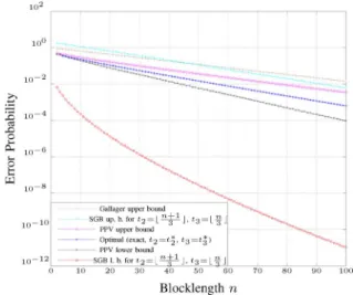
Fig. 12. Exact value of, and bounds on, the performance of an optimal code with codewords on the BSC with as a function of the block-length .
D. Application to Known Bounds on the Error Probability for a Finite Blocklength
We again provide a comparison between the performance of the optimal code to the known bounds of Section VI.
Note that the error exponents for codewords are (110) Moreover, for , if if if . (111)
Figs. 12 and 13 compare the exact optimal performance for and , respectively, with some bounds: the SGB upper bound based on the weak flip code used by Shannon et
al.,10the SGB lower bound based on the weak flip code (which
is suboptimal, but achieves the optimal and is therefore a generally valid lower bound), the Gallager upper bound, and also the PPV upper and lower bounds.
We can see that the PPV upper bound is tighter to the exact optimal performance than the SGB upper bound. Note, how-ever, that only the SGB upper bound exhibits the correct error exponent as is large enough. It is shown in [18] that, for going to infinity, the random coding (PPV) upper bound tends to the Gallager exponent for [6], which is of course not necessarily equal to for finite .
Concerning the lower bounds, we see that the PPV lower bound (metaconverse) is much better for finite than the SGB bound. However, for large enough, its exponential growth will approach that of the sphere-packing bound [15], which does not equal to either.
10The SGB upper bound based on the optimal code performs almost
Fig. 13. Exact value of, and bounds on, the performance of an optimal code with codewords on the BSC with as a function of the block-length .
Once more we would like to point out that even though the fair weak flip codes achieve the error exponent, they are strictly
suboptimal for every .
X. CONCLUSION
We have studied the optimal code design of ultrasmall block-codes for the most general binary discrete memoryless channel, the so-called binary asymmetric channel (BAC). For an arbitrary finite blocklength , we have analyzed the structure of optimal codes with two codewords.
We then have put special emphasis on the two most important special cases of binary channels, the Z-channel (ZC) and the
binary symmetric channel (BSC). For the ZC and for an arbitrary
finite blocklength , we have derived an optimal code design with four or less messages and we have conjectured an optimal code design with five messages. For the BSC and for an arbitrary finite blocklength , we have derived an optimal code design with two or three messages and we have conjectured an optimal code design with four messages.
Note that since the optimal codes we proposed do not depend on the cross-over probability of the channel, the optimal codes remain the same even if the channel is nonergodic or nonsta-tionary. Also note that the optimal weak flip codes are by defi-nition coset codes: the nonlinear code is always a coset of the linear code. However, they are not fixed compo-sition codes.
We have introduced a new way of generating these codes re-cursively by using a columnwise build-up of the codebook ma-trix. This column view of the codebook turns out to be a more powerful tool for analysis than the standard rowwise view (i.e., the analysis based on the codewords). We believe that the recur-sive construction of codes may be extended to a higher number of codewords and also to more complex channel models. In-deed, we have achieved some first promising results for the bi-nary erasure channel (BEC) [14]. Note, however, that in these more complex situations we might need a recursion from to
with a step-size .
We have also investigated the well known and commonly used code parameter minimum Hamming distance. We have shown that it may not be suitable as a design criterion for op-timal codes, even for very symmetric channels like the BSC.
Finally, we would like to point out that the family of weak flip codes defined in Section V (and in particular the subfamily fair weak flip codes) turns out to have many interesting properties. A first closer investigation of some of these properties and the relation of these codes to linear codes can be found in [14].
APPENDIXA
DERIVATIONSCONCERNING THEBAC
A. LLR Function
Proposition 40 (Properties of ):
1) If , then irrespective of
, , or .
2) is a nonincreasing function in for every
, :
(112)
3) For certain values of , the value of is
always nonnegative (or always nonpositive) for all and : if if depending on if (113)
4) is a nondecreasing function in for fixed
, , and .
5) is a nondecreasing function in for fixed
, , and .
6) For ,
(114)
Proof: These properties follow quite easily from the
def-inition of and the relations (1)–(3). We only
show a proof of the second property:
(115)
B. Alternative Proof of Theorem 23
Assume that the optimal code for blocklength is not a flip code. Then, the code has a number of positions where both codewords have the same symbol. The optimal decoder will ig-nore these positions completely. Hence, the performance of this code will be identical to a flip code of length .
We therefore only need to show that increasing will always allow us to find a new flip code with a better performance. In other words, Theorem 23 is proven once we have shown that
(116) Note that for the length- flip code of type
(117) we can derive two nontrivial length- codes
(118) Both of these codes happen to be (or at least be equivalent to) flip codes. We would like to remind the reader that is a flipped version of .
Since in the following we are going to compare different flip codes of either length or , we need to clarify our notation. So for the received vectors we use a superscript to de-note their length, and for the codewords , optimal decoding threshold , and the Hamming distance between a re-ceived sequence and the first codeword we use the superscript to denote their affiliation with the corresponding code of length . Hence, as shown in Theorem 24, the optimal ML de-cision rule for can be expressed as
if
if . (119)
The threshold satisfies . Note that when
, the decision rule is equivalent to a majority rule. Also note that when is even and , the decisions for and are equally likely, i.e., without loss of generality we then always decode to .
So let the threshold for be . We will now argue that the threshold for and (compare with (118)) must satisfy
(120) Consider first the code and assume by contradiction for
the moment that . Then, pick a received
with that (for the code ) is decoded to
. The received length- vector has
, i.e., it will be now decoded to . This, however, is a contradiction to the assumption that the ML
decision for the code was .
Second, again considering code , assume by
contra-diction that . Pick a received with
that (for the code ) is decoded to
. The received length- vector has
, i.e., it will be now decoded to . This, however, is a contradiction to the assumption that
the ML decision for the code was .
The same arguments also hold for the other code . Hence, we see that there are only two possible changes with respect to the decoding rule to be considered. We will next use
this fact to prove that .
The error probability of a length- code with two codewords and is given by
(121)
For , (121) can be written as follows:
(122)
(123)
(124)
Here, in (123) we use the fact that
and ; and in (124) we combine the
terms together using the definition of according to (26) (and (118)).
We can now distinguish the two cases (120): i) If the decision rule for is unchanged, i.e.,
in (124) that contains some terms that will now be de-coded differently. We split this sum up into two parts:
(125)
Since we have assumed that , we know
that for all with the
length-received vector has
and will be decoded to . Hence, we must have (126) Hence, we have (127) (128) (129)
ii) If the decision rule is changed such that , we need to take care of the second summation in (124)
that contains some terms that will now be decoded differ-ently. Again, we split this sum into two parts:
(130)
Since we have assumed that , we know
that for all with the
length-received vector has
and will be decoded to . Hence, we must have (131) The rest of the argument now is analogous to Case (i).
This proves that . The remaining
proof of is similar and omitted.
We remark that while in general ,
we only achieve equality if is even and .
The reason why we show this long derivation in addition to the compact proof given in Section VII-A is the expression (124) that explicitly states the error probability as a function of the ML decoder threshold. In the sequel of (124), we had to make a case distinction depending on what the correct ML de-coder looks like. In the proof of Theorem 25 in the following section, we will assume that the decoder is fixed, which will allow us to make even better use of (124).
C. Proof of Theorem 25
In order to derive the error probability expressions for and , we use the flip code and add either a column
or , respectively. Moreover, we assume that is decoded using the same fixed decoder threshold . Note that since we are using a similar approach as in Appendix A-B, we also apply the notation introduced there, i.e., we use a superscript to denote length and affiliation.
Following the same structure as in (124), we write the error probability of for the given decoding rule as follows:
(133)
Similarly, we can express the error probability of :
(134)
(135)
Subtracting (135) from (133) then yields
(136)
(137)
(138)
(139)
(140)
where in (139) we make use of our assumption that is decoded also using the same threshold .
Hence, we see that unless , in which case the
differ-ence is always zero, can only be
zero if
(141) From the definition of the log-likelihood ratio, we see that if we fix , then there exists at most one such that (141) is satisfied. The same is true if we fix and search for an .
APPENDIXB
DERIVATIONSCONCERNING THEZC
A. Proof of Theorem 30
Consider a general codebook matrix with codewords . Considering Remark 6, we can assume without loss of generality that
(142) and that all ones of the first codeword are in the last positions, i.e.,
(143) We are going to show that an optimal codebook must satisfy
.
We note that for any with
, and for every codeword , ,
the conditional channel law can be expressed as
(144) where denotes again the indicator function, and where we make explicit use of the shape of (143), the structure of the
considered received vector , and the assumption (142). Note that the value of (144)—if positive—only depends on via its Hamming weight. Hence,
(145) (146) where (146) follows from (142). Since when transmitting , the received sequence cannot have any ones in the first positions, this now shows that the optimal decoding region for the first codeword is
(147) which yields the conditional success probability
(148) Hence, we see that independently of the choice of . If we choose , though, then the size of is min-imized, i.e., many vectors that belong to for will be moved to some other decoding region , . This move will increase the success probabilities of the cor-responding other codewords (because the success probabilities will contain more terms in their corresponding sum over all ). Hence, since remains constant, the total suc-cess probability is increased.
Note that this increase is strictly larger than zero if there exists some other codeword that has one or more ones in the last positions.
B. Proof of Theorem 31
The proof of Theorem 31 is based on an exact expression of the average success probability as a function of the numbers of candidate columns . The problem is then transformed into an optimization problem.
We first consider the easier case of . By Theorem 30 and because the all-zero column can be ignored (based on the argument used in the proof of Theorem 23), we can restrict our search to the candidate columns given in (28). Hence, for any
blocklength , with , consider an arbitrary
codebook and, without loss of generality, assume that (149) Moreover, note that
(150)
and (because ) that .
The decoding region of the first codeword is just the all-zero
vector with .
Defining and using a derivation similar to
(145)–(147), we further realize that
(151) and
(152) Finally, the remaining belong to :
(153)
(154) with
(155) (156) Hence, the average success probability for a codebook
with and is
(157) The proof for the case is now completed by showing that the average success probability (157) is maximized by the
choice . Note that the exact choice of and is
irrelevant as long as .
In the case of , we cannot only rely on the candidate columns in (29), but unfortunately need to consider totally seven candidate columns:11
(158)
We use to describe an arbitrary code,
and again, without loss of generality, assume that
(159) Also note that
(160) (161) (162) (163)
and, as a result, and . Again, we
investigate the decoding regions with the corresponding success probabilities.
11By the argument shown in the proof of Theorem 23 and by Theorem 30,
The first two decoding regions are very similar to the case of and yield (164) Then, we have (165) with (166) The fourth decoding region is more complicated. It can be written as (167) where (168) Hence, (169) (170) (171) (172) where (173) and (174)
Hence, the average success probability for a codebook
with and is
(175) and is maximized for
(176) Furthermore, it can be shown that the optimum is unique for even , while there are also other solutions for odd .
C. Proof of Theorem 34
We apply (157) and (175) to the weak flip code of type .
Corollary 41: On a ZC, for or , and for any , the optimal decoding regions for the weak flip
code of type , , for , are
(177)
(178)
(179) (180) The corresponding average success probabilities are
(181) (182) Note that all received sequences in have zero proba-bility of occurring in the situation of because the code does not contain the all-one codeword. Therefore, we do not need to include them into any decoding region for .
We start with and recall that we can restrict our search to the seven columns given in (158). To prove Lemma 34, we ap-pend an additional bit to all four codewords of as follows: (183)
where and where and are given in (26)
with . We denote12 this new code by
. We now need to establish the decoding regions for the new code . If we simply extend the decoding regions
12Note that again we use a proof technique that uses a given code to create a
new code by adding a column to the codebook matrix. We therefore again use the notation introduced in Appendix A-B, i.e., we use superscripts to clarify length and affiliation.
given in (177)–(180) by one bit, , for , then we retain the same success probability because
(184) (185) (186) However, it is quite clear that these regions are in general no longer the optimal decision regions for . So the question is how to fix them to make them optimal again (and thereby also finding how to optimally choose ).
First note that if , adding a 0 to the received vector will not change the decision because 0 is the success outcome anyway. Similarly, if , adding a 1 to the vector will not change the decision .
Second, we claim that even if , all received
vec-tors still will optimally be decoded to .
To see this, we have a look at the four cases separately:
1) : The decoding region only contains
one vector: the all-zero vector. We have
(187)
independently of the choices for , .
Hence, we decide for .
2) : All vectors in contain ones in
po-sitions that make it impossible to decode it as or . On the other hand, obviously is less likely
than , i.e., we decide .
3) : All vectors in contain ones in
po-sitions that make it impossible to decode it as or . On the other hand, obviously is less likely
than , i.e., we decide .
4) : All vectors in contain ones in
posi-tions that make it impossible to decode it as , ,
or . It only remains to decide .
So, it only remains to investigate the decisions made about the
vectors in if . Note that we do not need
to bother about as it is impossible to receive such a vector. For , 2, or 3, if , the received vectors in will change to another decoding region not equal
to because .
1) : If we assign these vectors (actually, it has only one) to the new decoding region , the conditional success probability for is increased by
(188) (189) (190) where if if . (191)
Note that we only have a positive increase in the success probability if . Similarly, we compute
(192) (193)
From , we see that gives the highest
increase, followed by and then . Hence, in order to represent this choice of ordering, we rewrite (190), (192), and (193) as follows:
(194) (195) (196)
2) : In this case, only yields a nonzero
additional conditional success probability
(197)
(198) (199)
3) : Again, only yields a nonzero
addi-tional condiaddi-tional success probability
(200) (201)
For , we can now conclude that the unique best
solution for the choice of , yielding the largest increase in success probability in (194), (195), (196), (199), and (201), is as follows:
(202)
which corresponds to . This choice will lead to a total suc-cess probability increase of
(203) (204)
If is even and , then . In this case, still
yields the largest increase in success probability, but it is not anymore the unique choice to do so.