邊界效應對高階雷射模態之產生和雷射激發水柱之噴濺的影響

國立交通大學

電子物理研究所

博士論文

邊界效應對高階雷射模態之產生和雷射

激發水柱之噴濺的影響

Boundary effects on generation of

high-order laser modes and morphology of

laser-induced water jets

研 究 生 : 陳建至

指導教授 : 陳永富 教授

中華民國 102 年 5 月

邊界效應對高階雷射模態之產生和雷射激發水柱之噴濺的影響

Boundary effects on generation of high-order laser modes and morphology

of laser-induced water jets

研 究 生 : 陳建至

Student : Ross C. C. Chen

指導教授 : 陳永富

Advisor : Yung-Fu Chen

國 立 交 通 大 學 電 子 物 理 學 系

博 士 論 文

A Thesis

Submitted to Department of Electrophysics College of Science

National Chiao Tung University in partial Fulfillment of the Requirements

for the Degree of PhD

In Electrophysics

May 2013

Hsinchu, Taiwan, Republic of China

邊界效應對高階雷射模態之產生和雷射激發水柱之噴

濺的影響

學生 : 陳建至 指導教授 : 陳永富

國立交通大學電子物理學系博士班

摘要

本文的第一部分，利用半導體雷射VCSEL類比研究橫向邊界下的橫向高階模 態，並且從近場至遠場的觀察，研究橫向模態出光的特性和方向性。相較於微腔 體發光元件之出光特性的研究，利用VCSEL可以更直接的觀察到其模態的空間演 進。從研究結果中，我們證明了近場橫向模態和出光的方向性並非絕對一對一的 關係。當近場橫向模態有著圖像上顯著的差異，其遠場仍有可能具有大致相同的 方向性。更進一步，我們藉由量子彈子球檯的模型和近軸光學的繞射來理論分析 觀察到的實驗結果。 第二部分，我們對雷射激發水柱之噴濺的形成作了深入的研究。將雷射垂直 聚焦入射於水面之下，利用高速攝影觀察水面上之噴濺的行為，並針對其結構和 形成機制做了細節的探討。在水柱於空間行進的演化中，水柱中間會產生一個氣 泡，並且在適當的雷射聚焦深度下，此氣泡中會包含一顆水滴。此外，由於雷射 產生的電漿具有很大的動能平行於入射方向，因此當我們將雷射水平入射聚焦於 水中時，水面的噴濺將不再是柱對稱結構，具有平面結構的特徵變化。 i

Boundary effects on generation of high-order laser

modes and morphology of laser-induced water jets

Student: Ross C. C. Chen Advisor: Prof. Yung-Fu Chen

Institute and Department of Electrophysics

National Chiao-Tung University

Abstract

In this work, we investigate the high-order laser modes by a large-aperture VCSEL in different shapes of transverse confinement. VCSELs bear the potential to allow for directly observing the transverse modes and its free space propagation. Additionally, the light emitted from VCSEL is meaningful for studying the time diffraction from a high-order quantum mode. The experiment is reconstructed very well by theories of quantum billiard and Fresnel diffraction. We show that the far-field directional emission from a microcavity is just a necessary not sufficient condition for the emergence of a superscar mode.

In next part, we investigate the laser-induced liquid jet. A pulsed laser is vertically focused into a tap water to induce a water jet on a flat water surface. The water jet is observed by a high speed camera and the mechanism is discussed in detail. In the temporal evolution of the water jet, there is an air bubble with a water drop inside formed in the water jet. Additionally, we horizontally focus the laser beam into the water and observe the water jet. This water jet shows a sheet features.

誌謝

Acknowledgement

進入實驗室是在大學三年級的時候，之後逕讀博士到畢業共六年的研究生涯， 其中，曾一度隨著自己的任性與興趣而徘徊或中斷，但最後終於完成了它。這六 年中，非常感謝陳永富老師對我的提攜、關懷與照顧。在這浩瀚無垠的知識，永 無止盡求學之道，能遇到兼具實作經驗及深厚理論分析能力的陳老師，指引著我 如何做研究。陳老師的因材施教更讓學生能夠對於自己的長處有所發揮，並學習 獨立思考和自我要求。與陳老師互動討論，著實讓我受益良多。另一個要感謝的 是黃凱風老師。學識淵博的黃老師，總是能以清晰的物理圖像解釋實驗及理論結 果，並給予關於研究更好的建議，更是讓我欽佩不已。總之，縱有千言萬語，也 無法表達我對這兩位老師的感激之情。 再來要感謝的是在研究求學期間給予我無限支持及鼓勵的家人及朋友，感謝 我的父親陳振芳教授對我的研究和論文寫作的幫助，感謝母親讓我在每一天的研 究完回家時能有一頓豐盛的晚餐，並時時關心我的狀況；感謝我阿姨和外婆對我 的呵護；感謝陸爸爸陸媽媽一家對我的關愛及鼓勵。這些重要的人陪伴我走過無 數的困頓、煩憂。 最後，感謝蘇老大在實驗上的指導和獨到的見解，感謝教導我做實驗的建誠 和彥廷學長，感謝他們的熱心分享所學。非常感謝實驗室的同仁興弛學長、亭樺 學姊、依萍學姊、雅婷學姊、哲彥學長、仕璋學長、漢龍學長、小江、文政、易 純、威哲、毅帆、毓捷、郁仁、舜子、國維、威霖、凱勝、容辰、段必、小佑、 及政猷，使我的研究所生涯更豐碩。 誠摯感謝實驗室的各位帶給我的一切，讓我能砥礪自我並更向前邁進。 iii

Content

Abstract (Chinese)

i

Abstract

ii

Acknowledgement

iii

Contents

iv

List of Figures

vi

Chapter 1. Introduction ... 1

1.1 High-order transverse modes ... 1

1.2 VCSEL – vertical cavity surface emitting laser ... 3

1.3 Jet formation – Laser-induced water jet ... 10

Reference ... 13

Chapter 2. High-order lasing mode and free space propagation of large-aperture VCSELs ... 18

2.1 Large-aperture square VCSEL ... 18

2.1.1 Theoretical analysis ... 18

2.1.2 Experimental setup ... 24

2.1.3 Results and discussion ... 26

2.2 Large-aperture equilateral-triangular VCSEL ... 33

2.2.1 Theoretical analysis ... 33

2.2.2 Experimental setup ... 38

2.2.3 Results and discussion ... 39

Reference ... 52

Chapter 3. Laser-induced breakdown beneath a flat water surface – Vertical focusing ... 54

3.1 Experimental setup ... 54

3.2 Results and discussion ... 59

3.2.1 Thin jet, thick jet, and crown formation ... 59

3.2.2 Temporal evolution of laser-induced water jet ... 73

Reference ... 80

Chapter 4. Laser-induced breakdown beneath a flat water surface – Parallel focusing ... 83

4.1 Laser-induced elongated bubble in infinite surrounding ... 84

4.2 Experimental setup ... 86

4.3 Results and discussion ... 88

Reference ... 101

Chapter 5. Summary and Future works ... 103

Reference ... 106

Appendix A ... 107

Appendix B ... 111

Reference for Appendix ... 117

Curriculum Vitae ... 119

Publication List... 120

List of Figures

Chapter 1

Fig. 1.1 Schematic diagram of a gain-guided VCSEL with ion implantation regions

to confine the injection current as the effective active transverse region [13, Fig. 1.9]. ··· 7

Fig. 1.2 Schematic diagram of airposted VCSEL (index-guided structure) [14, Fig.

1.]. ··· 8

Fig. 1.3 Schematic diagram of an index-guided VCSEL with oxide aperture [17, Fig.

6.]. ··· 9

Chapter 2

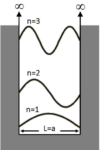
Fig. 2.1 Eigenfunctions with Eigenvalues n=1, 2, and 3 of 1D infinity potential well.

··· 21

Fig. 2.2 Low order eigenstates and a slight high-order mode (30, 30). We can expect

that properties of classical periodic orbits can not manifest and construct only by the conventional eigenstates even in the correspondence limit of large quantum numbers. ··· 22

Fig. 2.3 Stationary coherent states of , , 20,20p qφ( , )x y

Ψ with different

(

p q, ,φ

)

. The φ is set to be 0 to π and the values of

(

p q are ,

)

( )

_{1,1 ,}

( )

1,2 , and

( )

2,2 . ··· 23

Fig. 2.4 The schematic experimental setup for observing the near, far field, and the

free space propagation of VCSELs. ··· 24

Fig. 2.5 Schematic of the large-aperture square VCSELs device structure. ··· 25 Fig. 2.6 (a) The Bouncing-ball lasing mode at temperature 275K; (b) superscar

lasing mode (1,1) at temperature 260K. The far-field patterns (a’), and (b’) correspond to (a), and (b), respectively. ··· 28

Fig. 2.7 (a) The theoretical Bouncing-ball mode; (b) superscar mode (1,1). The

far-field patterns (a’), and (b’) correspond to (a), and (b), respectively. ···· 29

Fig. 2.8 The free-space propagation of a bouncing-ball near field. The experimental

results are shown in first and third rows and the theoretical results are shown in the second and forth rows. ··· 31

Fig. 2.9 The free-space propagation of a diamond-like superscar near field. ··· 32 Fig. 2.10 (a) Some eigenstates of equilateral-triangular 2D infinity potential well

( ) , ( , )

C m n x y

Φ . (b) Some eigenstates of equilateral-triangular 2D infinity potential well ( ) , ( , ) S m n x y Φ _{. When m=2n,} ( ) , ( , ) 0 S m n x y Φ = . ···35, 36

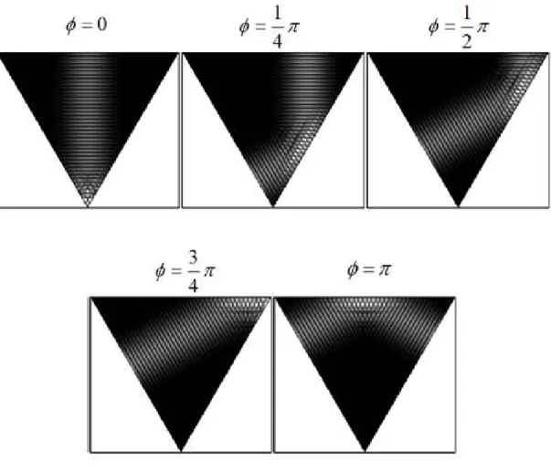
Fig. 2.11 Stationary coherent states of _Ψ42,20+ ( , ;1,0, )x y φ _{with different}φ_{. ··· 37}

Fig. 2.12 Schematic of the large-aperture equilateral-triangular laser device structure.

··· 38

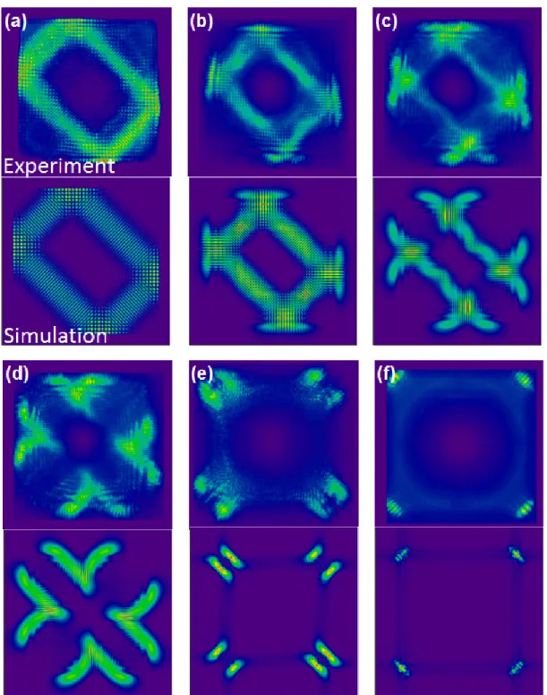
Fig. 2.13 Experimental near-field morphologies: (a) honeycomb eigenmode, (b)

cane-like superscar (1,0) mode, (c) superscar (1,1) mode. The far-field patterns (a’), (b’), and (c’) correspond to (a), (b), and (c), respectively. ···· 43

Fig. 2.14 Theoretical near-field morphologies: (a) honeycomb eigenmode, (b)

cane-like superscar (1,0) mode, (c) superscar (1,1) mode. The far-field patterns (a’), (b’), and (c’) correspond to (a), (b), and (c), respectively. ···· 44

Fig. 2.15 The experimental and Theoretical far-field patterns from honeycomb pattern

(above) and superscar (1,1) mode (bottom) in near field. The morphology of the numerical patterns is enhanced. ··· 45

Fig. 2.16 Six points on one of the triangular of Magen David is connected with only

one touch. ··· 46

Fig. 2.17 Experimental and theoretical results of free-space propagation of the

honeycomb eigenmode. The experimental results are shown in first and third rows and the theoretical results are shown in the second and forth rows. ··· 48

Fig. 2.18 Experimental and theoretical results of free-space propagation of the

cane-like superscar _{(1,0) mode. The experimental results are shown in} first and third rows and the theoretical results are shown in the second and forth rows. ··· 49

Fig. 2.19 Experimental and theoretical results of free-space propagation of the

superscar _{(1,1) mode. The experimental results are shown in first and third} rows and the theoretical results are shown in the second and forth rows. ·· 50

Fig. 2.20 The formation about six points in the diffraction pattern of the experimental

results. ··· 51

Chapter 3

Fig. 3.1 (a) The Experimental setup. (b) The high speed camera of GX-3 which is

setup at the right down corner of Fig. 3.1(a). ··· 56

Fig. 3.2 The initial bubble shape with different laser energy. The frame rate is

10,000 fps and the time of each frame is labeled on the top. ··· 57

Fig. 3.3 The maximum bubble diameter with different laser energy. The solid line is

a guide for the eye. ··· 58

Fig. 3.4 A complete water jet is generated on a flat free surface with γ = 0.8. The

frame rate is 80,000 fps. In the pictures of surface sinking, the exposure time is set to 1μs. ··· 60

Fig. 3.5 The numerical simulation and curvature schematic of the surface depression

are shown. The z and r of cylindrical coordinate are normalized to the Rmax

of the bubble. ··· 62

Fig. 3.6 A surface schematic of the circular ring-shaped crater is shown, which is

generated around the thin jet during the surface depression induced by the downward collapse bubble. ··· 63

Fig. 3.7 The frame rate is 80,000 fps as same as Fig. 3.4. Figures 3.7(a) and (c)

illustrate the non-crown formation when γ-value is smaller than 0.5 and larger than 1.1, respectively. Figure 3.7(b) shows another structure of the crown formation as compared to Fig. 3.4. This crown is denoted as unstable crown formation. ··· 65-67

Fig. 3.8 (a) The Schlieren photograph about the interaction between the shock wave

emitted from the bubble and the free surface [13, Fig. 5]. (b) A zero pressure region is formed between the bubble and the bottom of the thin jet [3, Fig. 4(g)]. ··· 69

Fig. 3.9 The structures of the thin jets and crowns with different γ-values which are

labeled on the left top of each image. The fame rate is 30,000 fps but the time interval between each frame is 0.166 ms. The arrow shows the orientation of the crown wall, which rotates counterclockwise to vertical direction when γ is increased from 0.5 to 1.02. ··· 71

Fig. 3.10 A typical result for the experimental result for the morphological variations

in the temporal evolution of the water jet generated by laser-induced breakdown at a depth of γ = 0.9. The time (in μs) is indicated at the bottom of each frame. ··· 75

Fig. 3.11 A typical result for the morphological variations in the temporal evolution

of the water jet generated at a depth of γ = 0.7. ··· 77

Fig. 3.12 A typical result for the morphological variations in the temporal evolution

of the water jet generated at a depth of γ = 1.04. The time (in μs) is indicated at the bottom of each frame. ··· 78

Fig. 3.13 Dependence of the pinched altitude H of the crown-shaped water jet on the

depth parameter γ in the range of 0.6-1.1. The time (in μs) is indicated at the bottom of each frame. ··· 79

Chapter 4

Fig. 4.1 The oscillation of an elongated bubble in infinite surrounding. The frame

rate is 100,000 and the exposure time is 1μs. ··· 85

Fig. 4.2 The schematic experimental setup for observing the water jet on the free

surface. Laser is horizontally focused into the water. ··· 87

Fig. 4.3 The water jet for γ = 1.18. The major axis of the bubble is parallel to the

water surface. The frame rate is 30,000 and the exposure time is 10μs. ···· 90

Fig. 4.4 The water jet for γ = 0.76. The time (in μs) is indicated at the bottom of

each frame. The top of the thick jet shows an asymmetry crown-shape water jet. ··· 91

Fig. 4.5 (a) The water jet for γ = 0.73. The exposure time is 10μs and the time (in μs)

is indicated at the bottom of each frame. The thin jet analogously rotates like drill. (b) The zoom-in pictures around the surface depression. The frame rate is 50,000 and the shutter speed is 3μs. The time (in μs) is indicated at the bottom of each frame. ··· 95

Fig. 4.6 The breakup of a water jet induced by vertically focusing the laser beam

beneath the free water surface. The waving on the water jet is cylindrical symmetry and the water jet gradually breaks up into several drops. Additionally, the breakup of the thin part of the water jet has similar result. ··· 96

Fig. 4.7 (a) The vibrations on the thin jet with directions on major and minor axes

are unmatched to each other. (b) The schematic of the circular polarized of an electromagnetic wave. ··· 97

Fig. 4.8 The water jet for γ = 0.63. The exposure time is 10μs and the time (in μs) is

indicated at the bottom of each frame. The thin jet is pulled outward by the two arms and forms a sheet structure. ··· 98

Fig. 4.9 A sheet thin jet with shape in non-isosceles triangle is generated when the

laser is focused with focus length in 120mm. As we can see in the first frame, the shape of the elongated bubble is twist due to the energy distribution around the focus volume induced by increasing the focus length. ··· 99

Fig. 4.10 The water jet for γ = 0.55. The exposure time is 10μs and the time (in μs) is

indicated at the bottom of each frame. The thick jet shows a sheet structure and gradually shrinks back to a cylinder-like structure. ··· 100

Chapter 5

Fig. 5.1 A laser-induced water jet is generated by vertically focusing the laser beam

beneath a free surface with a lateral equilateral triangular boundary inserted below the free surface. There are three arms forms on the crown, which are perpendicular to the three edges of the triangle, respectively. ··· 105

Appendix

Fig. B.1 The geometry of scheme chosen for constructing the model of pulsation

bubble beneath a free surface. The normal vector points out from the fluid domain. The azimuth angle is θ . ··· 116

Chapter 1. Introduction

The effects of boundaries are popular in sciences, technology applications, and even in our daily life. In quantum mechanics, the potential wells of boundaries quantize the energy states and determine the wave function. The general types of potential well are infinity potential and quantum harmonic oscillator. The wave function of these potential well are the types of the few quantum-mechanical systems for which an exact, analytical solution is known. In classical mechanics, boundary is important for studying the properties of system. For example, a thermodynamic system is defined by boundaries or walls of specific natures, together with the physical surroundings of that region, which determine the processes allowed to affect the interior of the region.

In this work, we studied the boundary effects on transverse modes in optics and the laser-induced water jet in fluid mechanics, and firstly, in this chapter, we briefly review the previous works in these fields.

1.1 High-order transverse modes

Resonant cavity is essential to laser or other optical devices and determines the special feature of the emitted light, e.g. power, beam directionality, quality factor, output spectrum. In microdisk laser, for achieving low threshold, the shape of cavity can be designed in circular disk or cylinder to achieve the high-Q modes due to the well-known whispering-gallery mode in a circular-shaped planar cavity [1-3]. In addition to the threshold, integration of microdisk laser into an optoelectronic system

will require coupling the light from microdisk laser to outer system like fiber or another microdisk. The well control directional emission is necessary for high-Q microdisk applications.

The general method to implement a directional emission is the shape deformation. Asymmetric resonant cavities slightly deformed from perfect symmetry cavities (e.g. circular or spherical cavities) lead to partially chaotic ray dynamic. The ray in such deformed cavity can not be completely confined by the total internal reflection of the boundary, and finally leaks at an artificial gap on the cavity to achieve the desired directional emission. Recently, the research on shape deforming, e.g., a deformed circular cavity by J. U. Nockel & A. Douglas Stone [4,5], G. D. Chern 2003 [6], and J. Lee 2008 [7]; a deformed square cavity by Tao Ling [8]; corner-cut square cavitiy by Chung Yan Fong [9]. In addition to the method of deformation, stadium shape is another way to implement the directional emission, which is classified to irregular billiard and studied in the fields of classical and quantum chaos [10]. The stadium resonator consists of two half-circles connected by two straight side walls. In classical billiard model in which classical particle moves freely and bounces elastically with no energy loss, there are two types of orbits: stable periodic orbit (PO) and unstable PO. Stable POs form a close loop and always exist in a regular billiard because of their high symmetry. On the other hand, unstable POs are determined according to that the PO is diverged and can not form a close loop when the trajectories of the PO have slightly dislocation or shift. For example, in a stadium resonator, the diamond periodic orbit is an unstable PO and the bouncing ball between the straight side walls is a stable PO. In a quantum model, interference patterns of wave functions localized around the unstable periodic orbits are called "scars" named by Heller [11]. In addition to scars, wave functions localize on the perturbation stable

periodic orbits are so-called “superscars”, which was originally used by Heller [11] to make a difference with scar.

The main drawback in the studies of microcavity or microdisc laser is that the transverse mode can not be directly measured. Generally, the transverse modes of a microdisc laser are theoretically constructed from the directional emission of output in experiment. In this article, vertical cavity surface emitting lasers named VCSELs are used to study the high-order transverse modes in certain shapes of boundaries. As shown in next section, VCSELs can be analogously investigated the transverse modes in a microcavity and the output emitted light from VCSEL bears the potential to allow for directly measuring the transverse modes and directional emissions.

1.2 VCSEL – vertical cavity surface emitting laser

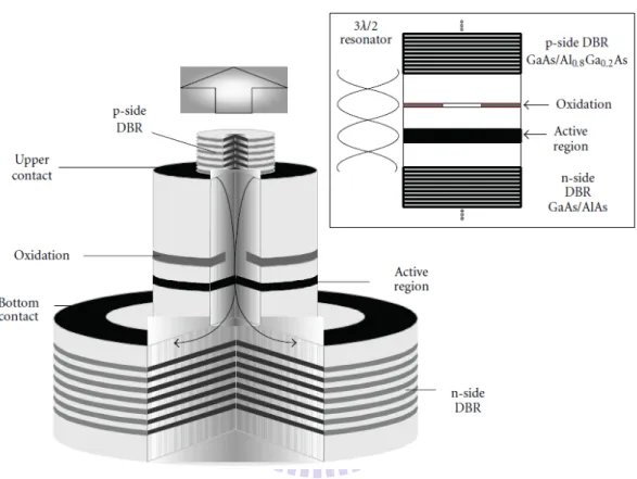
Vertical-cavity surface-emitting lasers (VCSELs) are made by sandwiching a light emitting layer between two highly reflective mirrors. The light emitting layer is generally composed in multi-quantum layer for high gain efficiency and the high reflective mirror can be dielectric multilayered or distributed Bragg reflectors (DBRs).

The transverse confinement of optical field and electrical current is important for designing VCSELs. Generally, there are three types to confine the transverse optical field: gain guiding, index guiding, or antiguiding mechanisms. In Fig. 1.1, gain guiding is generally achieved by ion implantation into the DBR to control the flow of the injection current into the active layer [12,13]. However the configuration of ion-implanted region can not well define the diffusion of carrier concentration along the transverse direction of the active layer. Additionally, it is hard to apply the ion implantation to the active region for well defining the current distribution because it

will increase the optical absorption loss of the VCSEL. Thus, at high power operation, the VCSEL with ion implantation can be excited high-order transverse modes due to the thermal lensing because of the non-well defined transverse confinement of the active layer. The other problem is the electrical resistivity of the DBR, which may increase the heat generation inside the laser cavity. The only benefit of this structure is planer configuration, which improves the simplification in fabrication process so the low production cost could achieve.

Compared to the gain-guided VCSELs, index-guided VCSELs have better transverse confinement of optical field. The index-guided VCSELs are implemented by inserting a material which has a low refractive index then the semiconductor of active layer to confine the optical field of transverse mode. This structure is similar to the waveguide of a fiber. Several types of index-guided VCSELs are implemented such as airposted, etched mesa and oxide aperture. These types have different mechanisms to confine the optical field and injection current as well as different production costs in fabrication process. The airposted VCSELs [14] as shown in Figure 1.2, the edge of active layer is direct contact with the outside air. The large difference in refractive index between the semiconductor material and the air provide very robust transverse confinement on optical field. But the roughness of the sidewall and the aperture-like structure from the active layer to the downside DBR increase the scattering and diffraction loss respectively. According to the research of waveguide, the larger the difference of refractive index between the materials of core and cladding layer the stronger confinement of optical field in the core, but conversely, the mode number will increase. Thus the single-mode operation is not stable in airposted VCSELs, especially at high injection current. Another type of index-guide VCSELs called oxide aperture VCSEL (Fig. 1.3) are now the most popular and promising devices for several applications such as short range communication, optical disk

readout head, laser printing, and sensor application [15-17]. For the confinement of optical field, effective refractive index between the oxide aperture and the surrounding semiconductor material can be controlled though the thickness of the oxide aperture and the location relative to the active layer. Additionally, the insulation of silicon oxide of oxide aperture forces the injection current though the aperture, which enhance the wall-plug efficiency [18]. As a result, the oxide aperture VCSELs have advantages on the well define of transverse lasing modes, extremely low threshold current [19], and low cost and high yield production of the oxidization procedure.

For analogously studying the direction emission from a transverse mode of a microcavity by VCSEL, we have to confirm the relation between the transverse mode of a microcavity and the transverse optical filed of VCSELs. The electric field of optical beams obeys the wave equation

(

2 2

)

(

)

2 0 _t x y z t, , : 0 µ ε∂ ∇ − Ε = ∂  . According to the waveguide theory, the electric fields with a predominantly z direction of propagation can be approximated as Ε

(

x y z t, , :

)

= Ε

( )

x y e, i k z( z −ωt), where

z

k is the wave vector along z-direction and ω is the angular frequency [20]. Although VCSELs have highly symmetric structure, the existence of anisotropy can break the degeneracy of transverse modes in two orthogonal polarizations, resulting in a split in oscillation frequency. Therefore, total electric field includes the two polarized states can be expressed as

(

, , :

)

( )

, i k z( z x, xt) ˆ x x x y z t x y e −ω a Ε = Ε +

( )

_, i k( z y, z yt) ˆ y x y e ay ω − Ε , (1.1)

where k and z x, k are the wave vector along z-direction, and the z y, ω is the angular i

frequency in i -polaried state. After separating the z component in the wave equation,

we are left with a two-dimensional Helmholtz equation in the two polarized states

(

)

(

)

(

)

(

)

2 2 2 0 , 2 2 2 0 , , 0 , 0 t x z x x t y z y y k x y k x y µ εω µ εω ∇ + − Ε =    ∇ + − Ε =    , (1.2) where 2 t

∇ means the Laplacian operator operating on the transverse x and y coordinates. Since the electric field in VCSELs experience total reflection on the lateral walls, transverse optical field at the boundary of cavity can be approximated as

( )

, _, 0

i x y _{x y}∈ℑ

Ε = with i x= or y . Obviously, transverse electric fields of VCSELs are thoroughly equivalent to eigenfunctions of 2D Schrödinger equation with infinity potential well of the same geometry. In other words, the transverse optical fields

( )

,

i x y

Ε _{of VCSELs can be used to analogously investigate the wave functions}

( )

x y,

y _{in two-dimensional (2D) quantum billiard. In our previous works [21], we}

have confirmed this important theoretical prediction by experiment.

Fig. 1.1 Schematic diagram of a gain-guided VCSEL with ion implantation regions to confine the injection current as the effective active transverse region [13, Fig. 1.9].

Fig. 1.2 Schematic diagram of airposted VCSEL (index-guided structure) [14, Fig. 1.].

Fig. 1.3 Schematic diagram of an index-guided VCSEL with oxide aperture [17, Fig. 6.].

1.3 Jet formation – Laser-induced water jet

In the next part of this work, we investigate the liquid jet formation. These studies are widely encountered in nature and various applications such as ink-jet printing, spray cooling, quenching and cutting of metal, liquid jet based needle-free injectors, DNA sampling, nuclear fission, powder technology [22-25]. On the other hand, jet dynamic investigates several physical properties of fluid, such as surface tension, viscosity, and non-Newtonian rheology. Almost all classical physics comes into play in the dynamic of jet, and still remains several challenging cases. In this article, we focus on the laser-induced liquid jet on a free surface. Free surface flows are almost the most beautiful and complicate phenomena encountered in fluid mechanics. This is especially true when a liquid surface is disturbed by a violent event beneath the free surface in the fluid domain or from the outside world to the fluid domain like an object impact or a reflecting shock wave.

When an object travels through a free surface of a fluid, a familiar jet formation exists, which is called Worthington jet [26] after the pioneering work on time-resolved imaging of A.M. Worthington. The object impacting on the free surface causes a crater on the free surface, and the collapse of this crater generates a vertical upward jet. Eruption of liquid jets from collapsing depressions has indeed been observed in a number of diverse instances, such as forcing the standing Faraday waves in a liquid surface [27], during the burst of bubbles [28], and tubular jet [29]. The tubular jet is formed in a tube when the tube is initially immersed in a tank of fluid and then suddenly released [29]. In addition to the fluid, a bed of fine, loose sand which nearly has no surface tension can also generate a remarkably different jet dynamics called granular jet when a particle falls and impacts into the sand [30].

Compared to the jet formed from a crater, a jet or splash forms on a free surface when an object is expanding very fast beneath a water surface such as material explosion which was studied extensively since World War II in the field of underwater explosions [31]. These studies, dealing with a large-size explosion bubble in underwater explosion, mainly focused on the bubble oscillation and the generation of spray on the free surface [31,32]. Recently, a small-scale cavitation bubble in millimeter size was used and the results showed more qualitative behaviors compared to the large-size explosion bubble for further theoretical simulations [33]. Understanding these behaviors is believed to shed light on the mechanisms of the erosion damages on a deformable surface caused by a nearby collapsing bubble [34,35]. Such a small-scale bubble was generally generated by using spark discharge [36] and these studies showed that, universally, an oscillating bubble develops into a toroidal shape during its collapse [33-35]. This shape evolution was reconstructed well in theoretical simulations [33-35]. In addition to the bubble, a liquid jet was seen to burst out from the free surface, and for a certain bubble depth, there emerged a thin jet followed by a markedly thicker jet and a circular crown-like jet perfectly connected on the shoulder of the thick jet transited to the thin jet [34,37].

The main drawbacks of the spark discharge and material explosive are the unavoidable influence of the electrodes and remained explosives on the dynamics of the bubble and liquid jet. In contrast, lasers have been shown to be useful and precisely controllable for generating a bubble by direct optical breakdown with pulsed lasers [38,39] or thermocavitation with CW lasers [40]. Several dynamics with different boundary systems were observed such as rigid wall for applications of erosion damages and fluid pumping [38,41,42], membrane or living cell for tissue engineering applications [43,44]. The oscillation times of a cavitation bubble near a rigid wall and free surface were investigated and compared with modified Rayleigh’s

model [45]. Very recently, a liquid jet on a flat free surface induced by a femtosecond pulsed laser was implemented in a new laser printing technique named film-free laser induced forward transfer (LIFT) to overcome the constraint of solid or liquid film preparation [46]. Furthermore, the laser-induced breakdown bears the potential to generate a more complex and flexible jet formation by controlling the shape of the bubble. K. Y. Lim et al. in 2010 [47] showed that complex bubble patterns can be generated using a holographic element in which the laser energy distribution is controlled by the patterns displayed on a spatial light modulator (SLM) acting as a phase object by a Fourier transform. As a result, bubble shaping and multiple bubble are achievable for inducing desired liquid jet. However, despite the great potential in future, there still remain several unknown mechanisms about the liquid jet and its evolution such as the crown-like structure on the thick jet [37]. The purpose in this article is to explore the detailed mechanisms and temporal evolutions of the laser-induced liquid jet.

Reference

[1] S. L. McCall, A. F. J. Levi, R. E. Slusher, S. J. Pearton, and R. A. Logan, “Whispering-gallery mode microdisk lasers,” Appl. Phys. Lett. 60, 289-291 (1992).

[2] Kerry Vahala, Optical Microcavities (World Scientific Publishing Co. Pte. Ltd. 2004).

[3] D. K. Armani, T. J. Kippenberg, S. M. Spillane, and K. J. Vahala, “Ultra-high-Q toroid microcavity on a chip,” Nature, 421, 925-928 (2003).

[4] J. U. Nockel, A. D. Stone, and R. K. Chang, “Q spoiling and directionality in deformed ring cavities,” Opt. Letts. 19(21), 1693-1695 (1994).

[5] J. U. Nockel and A. D. Stone, “Ray and wave chaos in asymmetric resonant optical cavities,” Nature, 385, 45-47 (1997).

[6] G. D. Chern, H. E. Tureci, A. D. Stone, R. K. Chang, M. Kneissl, and N. M. Johnson, “Unidirectional lasing from InGaN multiple-quantum-well spiral-shaped micropillars,” Appl. Phys. Lett. 83(9), 1710-1712 (2003).

[7] J. Lee, S. Rim, J. Cho, and C. M. Kim, “Resonances near the Classical Separatrix of a Weakly Deformed Circular Microcavity,” Phys. Rev. Lett. 101, 064101 (2008).

[8] T. Ling, L. Liu, Q. Song, L. Xu, and W. Wang, “Intense directional lasing from a deformed square-shaped organic–inorganic hybrid glass microring cavity,” Opt. Letts. 28(19) 1784-1786 (2003).

[9] C. Y. Fong and A. W. Poon, “Planar corner-cut square microcavities: ray optics and FDTD analysis,” Opt. Express, 12, 4864-4874 (2004).

[10] M. C. Gutzwiller, Chaos in Classical and Quantum Mechanics (Springer-Verlag, New York, 1990).

[11] E. J. Heller, “Bound-State Eigenfunctions of Classically Chaotic Hamiltonian Systems: Scars of Periodic Orbits,” Phys. Rev. Lett. 53, 1515-1518 (1984).

[12] Y. J. Yang, T. G. Dziura, T. Bardin, S. C. Wang, and Fernandez, “Continuous wave single transverse mode vertical cavity surface emitting lasers fabricated by Helium implantation and zinc diffusion,” Electron. Lett. 28(3), 274-275, (1992). [13] S. F. Yu, Analysis and Design of Vertical Cavity Surface Emitting Lasers (Wiley

Series in Lasers and Applications, 2003).

[14] H. Saito, K. Nishi, I. Ogura, S. Sugou, and Y. Sugimoto, “Room temperature lasing operation of a quantum dot vertical cavity surface emitting lasers,” Appl. Phys. Lett. 69(21) 3140–3142 (1996).

[15] T. H. Oh, D. L. Huffaker, and D. G. Deppe, “Comparison of vertical cavity surface emitting lasers with half-wave cavity confined by single- or double oxide apertures,” IEEE Photon. Technol. Lett. 9(7) 875–877, (1997).

[16] S. A. Blokhin, J. A. Lott, A. Mutig, G. Fiol, N. N. Ledentsov, M. V. Maximov, A. M. Nadtochiy, V. A. Shchukin, and D. Bimberg “Oxide-confined 850 nm VCSELs operating at bit rates up to 40 Gbit/s,” Electron. Lett. 45(10), 501-503 (2009).

[17] R. Sarzała, T. Czyszanowski, M. Wasiak, M. Dems, Ł. Piskorski, W. Nakwaski, and K Panajotov “Numerical Self-Consistent Analysis of VCSELs,” Adv. Opt. Tech. 2012, 689519 (2012).

[18] P. W. Evans, J. J. Wierer, and N. Holonyak, “AlxGa1–xAs native oxide based

distributed Bragg reflectors for vertical cavity surface emitting lasers,” J. Appl. Phys. 84(10), 5436–5440 (1998).

[19] G. M. Yang, M. MacDougal, and P. D. Dupkus, “Ultralow threshold current vertical cavity surface emitting laser obtained with selective oxidation,” Electron. Lett. 31, 886–888 (1995).

[20] J. D. Jackson, classical electrodynamics (Wiley, New York, 1975), Chap. 8. [21] K. F. Huang, Y. F. Chen, and H. C. Lai, and Y. P. Lan, “Observation of the wave

function of a quantum billiard from the transverse patterns of vertical cavity surface emitting lasers,” Phys. Rev. Lett. 89, 224102 (2002).

[22] H. P. Le, “Progress and Trends in Ink-jet Printing Technology,” J. Imaging Sci. Techn. 42(1), 49-62 (1998).

[23] J. Kim, “Spray cooling heat transfer: the state of the art,” Int. J. Heat Fluid Fl. 28, 753–767 (2007).

[24] S. Mitragotri, “Current status and future prospects of needle-free liquid jet injectors,” Nat. Rev. Drug Discov. 5, 543-548 (2006).

[25] L. R. Allain, M. Askari, D. L. Stokes, and T. Vo-Dinh “Microarray sampling-platform fabrication using bubble-jet technology for a biochip system,” Fresen. J. Anal. Chem. 371, 146–150 (2001).

[26] A. M. Worthington, A Study of Splashes (Longmans, Green and Co., London, 1908).

[27] B. W. Zeff, B. Kleber, J. Fineberg, and D. P. Lathrop, “Singularity dynamics in curvature collapse and jet eruption on a fluid surface,” Nature 403, 401-404 (2000).

[28] J. M. Boulton-Stone and J. R. Blake, “Gas Bubble bursting at a free surface,” J. Fluid Mech. 254, 437-466 (1993).

[29] R. Bergmann, E. D. Jong, J. B. Choimet, D. V. D. Meer, and D. Lohse, “The origin of the tubular jet,” J. Fluid Mech. 600, 19-43 (2008).

[30] S. T. Thoroddsen and A. Q. Shen, “Granular jets,” Phys. Fluids 13, 4-6 (2001). [31] R. H. Cole, “Underwater explosions” (Princeton, Princeton Univ. Press., 1948). [32] J. B. Keller and I. I. Kolodner, “Damping of underwater explosion bubble

oscillations,” J. Appl. Phys. 27, 1152-1161 (1956). 15

[33] A. Pearson, E. Cox, J. R. Blake, and S. R. Otto, “Bubble interactions near a free surface,” Eng. Anal. Bound. Elem. 28, 295–313 (2004).

[34] G. L. Chahine, “Interaction between an oscillating bubble and a free Surface,” J. Fluids Eng. 99, 709-716 (1977).

[35] P. B. Robinson, J. R. Blake, T. Kodama, A. Shima, and Y. Tomita, “Interaction of cavitation bubbles with a free surface,” J. Appl. Phys. 89, 8225-8237 (2001). [36] R. H. Mellen, “An experimental study of the collapse of a spherical Cavity in

Water,” J. Acoust. Soc. Am. 28, 447-454 (1956).

[37] A. Pain, B. H. T. Goh, E. Klaseboer, S. W. Ohl, and B. C. Khoo, “Jets in quiescent bubbles caused by a nearby oscillating bubble,” J. Appl. Phys. 111, 054912 (2012).

[38] W. Lauterborn and H. Bolle, “Experimental investigations of cavitation-bubble collapse in the neighbourhood of a solid boundary,” J. Fluid Mech. 72, 391-339 (1975).

[39] P. A. Quinto-Su, V. Venugopalan, and C. D. Ohl “Generation of laser-induced cavitation bubbles with a digital hologram,” Opt. Express 16(23), 18964-18969 (2008).

[40] J.C. Ramirez-San-Juan, E. Rodriguez-Aboytes, A. E. Martinez-Canton, O. Baldovino-Pantaleon, A. Robledo-Martinez, N. Korneev, and R. Ramos-Garcia, “Time-resolved analysis of cavitation induced by CW lasers in absorbing liquids,” Opt. Express 18(9), 8735-8742 (2010).

[41] A. Philipp and W. Lauterborn, “Cavitation erosion by single laser-produced bubbles,” J. Fluid Mech. 361, 75-116 (1998).

[42] R. Dijkink and C. D. Ohl, “Laser-induced cavitation based micropump,” Lab Chip 8(10), 1676-1681 (2008).

[43] Y. Tomita and T. Kodama, “Interaction of laser-induced cavitation bubbles with composite surfaces,” J. Appl. Phys. 94, 2809-2816 (2003).

[44] T. H. Wu, S. Kalim, C. Callahan, M. A. Teitell, and P. Y. Chiou, “Image patterned molecular delivery into live cells using gold particle coated substrates,” Opt. Express 18(2), 938-946 (2010).

[45] P. Gregorčič, R. Petkovšek, and J. Možina, “Investigation of a cavitation bubble between a rigid boundary and a free surface,” J. Appl. Phys. 102, 094904 (2007). [46] M. Duocastella, A. Patrascioiu, J. M. Fernández-Pradas, J. L. Morenza, and P.

Serra, “Film-free laser forward printing of transparent and weakly absorbing liquids,” Opt. Express 18(21), 21815-21825 (2010).

[47] K.Y. Lim, P.A. Quinto-Su, E. Klaseboer, B. C. Khoo, V. Venugopalan, C. D. Ohl, “Nonspherical laser-induced cavitation bubbles,” Phy. Rev. E 81, 016308 (2010).

Chapter 2.

High-order lasing mode and

free space propagation of large-aperture

VCSELs

In this chapter, we study the high-order transverse modes emitted from VCSELs. Square and equilateral triangular shapes of the aperture of VCSELs are studied in chapters 2.1 and 2.2, respectively. In each chapter, firstly, the theoretical model for constructing the near-field transverse mode is studied. Next, the experimental results analyzed with the simulations are discussed.

2.1 Large-aperture square VCSEL

2.1.1 Theoretical analysis

A 1D cavity with rigid wall of boundary can be modeled from the infinity potential well which is the most simple and well known system in every textbook of quantum mechanics [1,2]. The eigenfunction of Schrodinger equation in 1D infinity potential well is solved as a sinusoid wave (Fig. 2.1) in which n is the quantum number. 2 ( ) sin( ) n x _a n x_a π y = (2.1) 18

Because the orthogonal and separable properties between the x and y coordinates, the eigenstates of 2D planer square infinity potential well can be described below

_{1 2} 1 2

, ( , ) 2sin( )sin( )

n n x y _a n x_a n y_a

π π

y = (2.2)

Figure 2.2 displays some of the eigenstates with their quantum numbers labeled below each figure. The eigenstates of regular square shape are like a chessboard and distribute averagely over the space which don’t show any indications of localization on periodic orbits even the quantum number approaches infinity.

According to the correspondence principle, when the quantum number approaches infinity, the probability of wave function will agree with the classical limit. Nevertheless, the wave function doesn’t become to a particle in classical limit. The way to connect the wave in quantum and particle in classical, is used the coherent states. The idea of coherent states is the superposition of a set of eigenstates with different eigenvalues and certain phase relations between each eigenstates [3]. As a result, a moving particle can be represented by the superposition of time-variant Schrodinger solution. Extracting the stationary states from the result of superposition of time-variant Schrodinger solution, we can get a wave function associated with periodic orbits.

The stationary coherent states in square shape infinity potential well can be displayed as followed [4]:

[

]

1 , , , , ( 1 ) 0 1 0 1 ( , ) ( , ) 2 ( 1 ) 2 ( ) sin[ ]sin[ ] 2 M p q M iK N M _M K qN pK pN q M K K M M iK K M K x y C e x y pN q M K y qN pK x C e a a a φ φ φ y π π − + + − − = − = Ψ = + − − + =

∑

∑

(2.3) 19

Figure 2.3 displays the stationary coherent states , , , ( , )

p q N Mφ x y

Ψ with different

( , , )p qφ . Obviously, the two positive integers p and q are related to the number of collisions with horizontal and vertical walls, and the φ (0≤ ≤φ 2 )π is the wall position of specular reflection points [5].

Fig. 2.1 Eigenfunctions with Eigenvalues n=1, 2, and 3 of 1D infinity potential well.

Fig. 2.2 Low order eigenstates and a slight high-order mode (30, 30). The properties of classical periodic orbits can not manifest and construct only by the conventional eigenstates even in the correspondence limit of large quantum numbers.

Fig. 2.3 Stationary coherent states of , , 20,20p qφ( , )x y

Ψ with different

(

p q, ,φ

)

. The φ is set to be 0 to π and the values of

(

p q are ,

)

( )

_{1,1 ,}

( )

1,2 , and

( )

2,2 .

2.1.2 Experimental setup

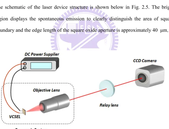
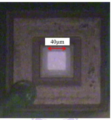
The experimental setup is shown in Fig. 2.4. The VCSEL device was placed in a cryogenic system with a temperature stability of 0.01 K in the range of 80–300 K. A DC power supplier (KEITHLEY 2400) with a precision of 0.005 mA is used to drive the VCSEL device. The near-field patterns were reimaged into a charge-coupled device (CCD) camera (Coherent, Beam Code) with an objective lens (Mitsutoyo, NA of 0.9). The far-field patterns are measured with a CCD placed behind a screen. The control parameters of the VCSEL in this experiment are the device temperature and pumping currents which are the important factors to affect the lasing transverse modes. The schematic of the laser device structure is shown below in Fig. 2.5. The bright region displays the spontaneous emission to clearly distinguish the area of square boundary and the edge length of the square oxide aperture is approximately 40 μm.

Fig. 2.4 The schematic experimental setup for observing the near, far field, and the free space propagation of VCSELs.

Fig. 2.5 Schematic of the large-aperture square VCSELs device structure.

2.1.3 Results and discussion

At temperature 275K, the lasing mode is shown in Fig. 2.6(a), generally, we call it the bouncing-ball mode. In numerical part, it can be roughly seem an eigenstate of square shape infinity potential well with very high order in horizontal quantum number and slightly deform. The eigenstate yn n_{1 2}, ( , )x y of square shape infinity

potential well mentioned in section 2.1.1 is shown below, 1 2 1 2 , ( , ) 2sin( )sin( ) n n x y _a n x_a n y_a π π y = (2.2)

According to the work by Chien-Cheng Chen in 2009 [6], the experimental bouncing-ball mode can be reconstructed by a linear combination of two eigenstates:

y40,11( , )sin(0.35 )x y π +y39,14( , )sin(0.35 )x y π (2.4)

The numerical simulation of the bouncing-ball mode is showed in Fig. 2.7(a).

When the operating temperture is decreased to 260K, the near-field of the VCSEL dramatically changes to a diamond-like pattern. About the discussion of numercal research in section 2.1.1, the superscars localized on the perodic orbits can be implemented by the coherent states as shown below [4].

1 , , , , ( 1 ) 0 1 0 1 ( , ) ( , ) 2 2 ( ) ( ( 1 ) sin[ ]sin[ ] 2 M p q M iK N M _M K qN pK pN q M K K M M iK K M _K x y C e x y qN pK x pN q M K y C e a a a φ φ φ y π π − + + − − = − = Ψ = + + − − =

∑

∑

(2.3) The Equation (2.3) is the form of traveling wave and the standing wave for experimental fitting is expressed as

1 ( )

,

0

2 ( ) ( ( 1 )

( , ; , , ) cos( )sin[ ]sin[ ]

2 M C M N M _M K K qN pK x pN q M K y C x y p q C K a a a π π φ − φ = + + − − =

∑

(2.5) , and the diamond-like superscar mode shown in Fig. 2.6(b) can be interpreted by

( )

36,10C ( , ;1,1,0.57 )

C x y π (Fig. 2.7(b)). (2.6)

As we can see, the near fields of the experiments are reconstructed very well by the model of quantume billiard.

Next, the experimental far fields of the two lasing modes in Figs. 2.6(a) and (b) are observed and shown in Figs. 2.6(a’) and (b’), respectively. The two far-field patterns are similar to each other. The far field from the superscar near-field pattern is a square with four points on the cornors of the square. Because the far field is related to the momentum distribution of the direction emision of the near field [7,8], we can see that the directions of the four points are parallel to the trajectory of the perodic orbit in near field. Base on the result of the far field of superscar mode, the far field of Fig. 2.6(a’) shows that the near field in Fig. 2.6(a) is not completely only a horizontal bouncing-ball mode. These results show that the far field could provide some information for determining the near field. In theoretical part, the far-field pattern is simulated by the method of Fraunhofer diffraction [7], as derived in Appendix A. The results are shown in Figs. 2.7(a’) and (b’) for the bouncing-ball near-field pattern (eq. (2.4)) and the diamond-like superscar (eq. (2.6)), respectively. There are great agreements between the experimental and numerical results both in the near-field and the far-field patterns.

Fig. 2.6 (a) The Bouncing-ball lasing mode at temperature 275K; (b) superscar lasing mode (1,1) at temperature 260K. The far-field patterns (a’), and (b’) correspond to (a), and (b), respectively.

Fig. 2.7 (a) The theoretical Bouncing-ball mode; (b) superscar mode (1,1). The far-field patterns (a’), and (b’) correspond to (a), and (b), respectively.

Based on the plenteous morphologies on the near-field and far-field patterns, we further explore the free space propagation from the near field to the far field and use the Fresnel diffraction derived in Appendix A to analyze the experimental results. In Fig. 2.8, the graph in monochrome is the experimental measurement, and the theoretical results are shown under each experimental result. The evolutions of the patterns are horizontal propagation and roughly follow the directions of the interference stripes of near-field patterns. According to the theoretical study, the standing wave is linearly combined by two opposite directional traveling waves. As a result, the interference stripes of near-field pattern will separate to two diffraction patterns in opposite directions as shown in the measurements and the theoretical results.

Compared to the free-space propagation of the bouncing-ball mode, the diamond-like superscar mode shows slight copious morphologies and apparent directions on the propagation of diffraction patterns, as shown in Fig. 2.9. Despite the direction of propagation parallel to the trajectory of the periodic orbit in near field, there are other directions which are not exist in the classical limit. This result is explained by the nature of interference of waves as follows. On the edge of square aperture, the two interference stripes overlap to each other and create another direction of interference pattern. This new interference pattern is parallel to the wall of square and will propagate parallel the boundary of the square, as shown in the sequence pictures (b) to (d) in Fig. 2.9.

Fig. 2.8 The free-space propagation of a bouncing-ball near field. The experimental results are shown in first and third rows and the theoretical results are shown in the second and forth rows.

Fig. 2.9 The free-space propagation of a diamond-like superscar near field.

2.2 Large-aperture equilateral-triangular VCSEL

2.2.1 Theoretical analysis

Compared to the square shape infinity potential well, the shape in equilateral-triangular is classically integrable but non-seperable system. Let three vertices of an equilateral-triangular to be set at (0, 0), (a/2, 3 / 2a ), and (-a/2, 3 / 2a ). The eigenstates in an equilateral-triangular infinity potential wall have been derived by several groups [9-11] and the wave functions of the two degenerate stationary states can be expressed as

( ) , ( , ) ₂16 cos ( )2₃ sin ( ) 2 3 3 3 2 2 cos (2 ) sin 3 3 2 2 cos (2 ) sin 3 3 C m n x y m n _a x m n y a a m n x n y a a n m x m y a a π π π π π π      Φ = _{ } + _{ } − _          + _ − _{  }         − _ − _{  }        (2.7) and ( ) , 2 16 2 2 ( , ) sin ( ) sin ( ) 3 3 3 3 2 2 +sin (2 ) sin 3 3 2 2 sin (2 ) sin 3 3 S m n x y m n _a x m n y a a m n x n y a a n m x m y a a π π π π π π      Φ = _− _ + _{ } − _         ₋            − _ − _           (2.8) ( ) , ( , ) C m n x y Φ and ( ) , ( , ) S m n x y

Φ have the following characteristics:

( ) , ( , ) 0 C m m x y Φ = , ( ) , ( , ) 0 S m m x y Φ = , ( ) ( ) , ( , ) , ( , ) C C m n x y n m x y Φ = −Φ , ( ) ( ) , ( , ) , ( , ) S S m n x y n m x y Φ = −Φ , ( ) ( ) , ( , ) , ( , ) C C m m n− x y m n x y Φ = Φ , and ( ) ( ) , ( , ) , ( , ) S S m m n− x y m n x y Φ = −Φ . (2.9) 33

Hence, the condition of m≥2n is required to keep all eigenstates to be linearly independent to each other. Figures 2.10(a) and 2.10(b) show some of the ( )

, ( , ) C m n x y Φ and ( ) , ( , ) S m n x y

Φ with their quantum number labeled below each picture. As similar to

the wave function in square shape potential well, the eigenstates do not manifest the localization on periodic orbits even if the quantum number approaches to infinity.

For the stationary coherent states in equilateral-triangular infinity potential well, first, the traveling wave states are represented from linear combination of eigenstates:

( ) ( ) , , , 2 ( , ) ( , ) ( , ) 16 2 2 exp ( ) sin ( ) 3 3 3 3 2 2 exp (2 ) sin 3 3 C S m n x y m n x y i m n x y i m n x m n y a a a i m n x n y a a π π π π ± Φ = Φ ± Φ      = _{ }± + _{ } − _          + _ − _{  }     2 2 exp (2 ) sin 3 3 n m x m y a a π  π    − _ − _{  }     _(2.10)

Next, the stationary coherent states associated with periodic orbits denoted by ( , , )p qφ in equilateral-triangular infinity potential well can be expressed as below [12,13]. 1 , /2 ( 1), ( ) 0 1 ( , ; , , ) ( , ) 2 M M iK M N N k p K N q M K K x y p q _φ − C e φ x y ± ± ± + + − = Ψ =

∑

Φ _(2.11)

A typical coherent states with ( , ) (1,0)p q = are showed in Fig. 2.11 in which the pattern with

4 π

φ = looks like an inverse cane.

Fig. 2.10 (a) Some eigenstates of equilateral-triangular 2D infinity potential well ( ) , ( , ) C m n x y Φ . 35

Fig. 2.10 (b) Some eigenstates of equilateral-triangular 2D infinity potential well ( ) , ( , ) S m n x y Φ _{. When m=2n,} ( ) , ( , ) 0 S m n x y Φ = . 36

Fig. 2.11 Stationary coherent states of Ψ42,20+ ( , ;1,0, )x y φ with differentφ.

2.2.2 Experimental setup

The experimental setup is the same as shown in Fig. 2.4. The VCSEL device was placed in a cryogenic system with a temperature stability of 0.01 K in the range of 80–300 K. A DC power supplier (KEITHLEY 2400) with a precision of 0.005 mA is used to drive the VCSEL device. The near-field patterns were reimaged into a charge-coupled device (CCD) camera (Coherent, Beam Code) with an objective lens (Mitsutoyo, NA of 0.9). The far-field patterns are measured with a CCD placed behind a screen.

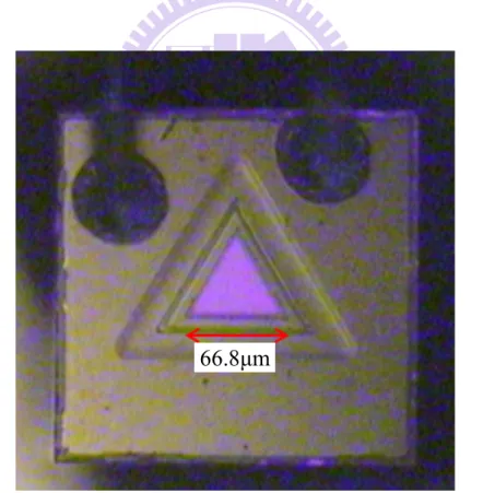
The schematic of the laser device structure with equilateral-triangular shape is shown in Fig. 2.12. The edge length of the oxide aperture is approximate 66.8 µm.

Fig. 2.12 Schematic of the large-aperture equilateral-triangular laser device structure.

66.8μm

2.2.3 Results and discussion

The experimental near-field morphologies are shown in Figs. 2.13(a)–(c) with different temperatures as labeled in each figure. Additionally, the corresponding far-field patterns for the honeycomb eigenmode, the cane-like superscar mode, and the superscar mode with ( , ) (1,1)p q = [14] are shown in Figs. 2.13(a’)–(c’). We can see that the near-field patterns for the honeycomb eigenmode and the superscar mode with ( , ) (1,1)p q = are conspicuously different to each other. However, their far-field patterns display fairly similar directional emission. The directional emission for a superscar mode can be easily traced from its localization in the near-field feature, as shown in section 2.1.3. Conversely, it is demanding to find the directional emission of a honeycomb lasing mode.

As described in section 2.2.1, the eigenstates for the standing waves are given by

( ) , ( , ) C m n x y Φ and ( ) , ( , ) S m n x y Φ as shown below: ( ) , ( , ) ₂16 cos ( )2₃ sin ( ) 2 3 3 3 2 2 cos (2 ) sin 3 3 2 2 cos (2 ) sin 3 3 C m n x y m n _a x m n y a a m n x n y a a n m x m y a a π π π π π π      Φ = _{ } + _{ } − _          + _ − _{  }         − _ − _{  }        (2.7) and ( ) , 2 16 2 2 ( , ) sin ( ) sin ( ) 3 3 3 3 2 2 +sin (2 ) sin 3 3 2 2 sin (2 ) sin 3 3 S m n x y m n _a x m n y a a m n x n y a a n m x m y a a π π π π π π      Φ = _− _ + _{ } − _         ₋            − _ − _           (2.8) 39

In terms of ( ) , ( , )

S m n x y

Φ , the experimental honeycomb pattern can be well

reconstructed with n=60 and m=6, as depicted in Fig. 2.14(a). On the other hand, the Superscar modes associated with classical periodic orbits can be analytically expressed with the coherent states.

1 , /2 ( 1), ( ) 0 1 ( , ; , , ) ( , ) 2 M M iK M N N k p K N q M K K x y p q _φ − C e φ x y ± ± ± + + − = Ψ =

∑

Φ (2.11)

And the standing wave CN M±, ( , ; , , )x y p qφ is represented:

CN M±, ( , ; , , )x y p q φ = Ψ+N M, ( , ; , , )x y p qφ ± ΨN M−, ( , ; , , )x y p qφ (2.12)

The experimental superscar pattern in Fig. 2.13(b) can be well reconstructed by

2 , ( , ; , , )

N M

C+ x y p q φ _{with N=36, M=9, and ( , , ) (1,0,0.23 )p qφ = π , as depicted in Fig.}

2.14(b). In the same way, the experimental superscar pattern in Fig. 2.13(c) is related to the theoretical solution C_{N M}+_, ( , ; , , )x y p q φ 2 _{with N=22, M=6, and}

( , , ) (1,1,0.3 )p q φ = π , as depicted in Fig. 2.14(c). The theoretical analysis of the far field can be implemented by combining the numerical near-field pattern and the equation of Fraunhofer diffraction. The calculation results of far field are shown in Fig. 2.14(a’) for honeycomb eigenmode, Fig. 2.14(b’) for superscar (1,0) mode, and Fig. 2.14(c’) for superscar (1,1) mode. The excellent agreements between the experimental and numerical patterns again confirm that the model of quantum system in infinity potential well is great important to analogically simulate the transverse lasing modes of the VCSELs, and this work was proposed in Ref. [15].

The experimental and theoretical results show that the near-field patterns for the honeycomb eigenmode and the superscar mode (Figs. 2.13(a) and (c) and Figs. 2.14(a) and (c)) are apparently different to each other. One spreads over the triangular space while the other one is localized on the periodic orbit with trajectory parallel to the three edges of the triangle. However, their far-field patterns display fairly similar directional emission with the angles at integral multipliers of 60_{. As a consequence,}

we confirm that the far-field directional emission is just a necessary not sufficient condition for the emergence of a superscar mode [15].

For detailed exploring the far fields of the honeycomb eigenmode and the superscar mode, the experimental results are redraw in Fig. 2.15 and the numerical patterns are calibrated by changing the index of square in CN M+, ( , ; , , )x y p q φ 2 to

0.8 , ( , ; , , )

N M

C+ x y p q φ _{for diminishing the contrast of the image and emphasizing the}

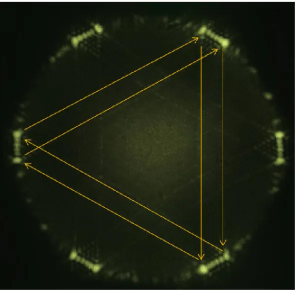
delicate morphology. There are two apparent differences between the far-fields in Fig. 2.15: the structures of the six points in each directional emission and the lines connected between the six points. Interestingly, these lines form two triangles with a shape in hexagram which is the well-known Magen David (Star of David).

In the far field of honeycomb eigenmode, there are two dots in each six directions of directional emission. As a result, there are total 12 dots in the far field. These dots can be explained by dividing the eigenstate ( )

, ( , )

S m n x y

Φ into three parts, each part is familiar to the eigenstates of a rectangle-shape infinity potential well. The three parts are as listed:

2 2 sin ( ) sin ( ) 3 3 m n x m n y a a π  π   ₊  ₋         , 2 2 sin (2 ) sin 3 3 m n x n y a a π  π   ₋          , and 2 2 sin (2 ) sin 3 3 n m x m y a a π  π   ₋         . 41

As shown in the section 2.1.3, the far field emitted from a rectangle-shape aperture VCSEL has 4 points on each directional emission. Based on this result, the 12 dots and its locations in the far field of a honeycomb near-field pattern are apparently reasonable.

Despite the 12 dots, the lines in Magen David can not get well explain from the results of the far fields emitted from a rectangle-shape aperture VCSEL. Actually, the lines are not real line but the interference patterns, and amazingly, the lines used to connect the six dots form one of the triangular in Magen David with a close loop (one touch drawing), as shown in Fig. 2.16. The detailed formation about this line is related to the superposition of the wave function for constructing the near-field transverse modes. For example, a summation of a group of sin waves to create a sinc function, because the number of the sin waves in the group is finite, there will exist some fluctuations between the peaks of sinc function. As a result, in the far field of VCSELs, it usually exist some interference-line patterns connected between each dots [6,7,16].

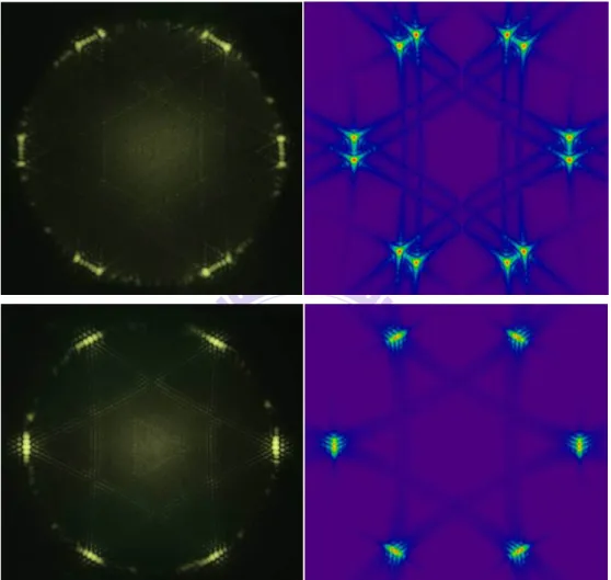
Based on the explanation of the Magen David emitted from honeycomb near-field pattern, the Magen David in the far field of a superscar mode (1,1) is explained as follows. The locations of the 12 dots are related to the quantum numbers of the eigenstates as confirmed by the far field of a rectangle-shape aperture VCSEL. When a group of eigenstates with different eigenvalues is combined to generate a coherent state CN M+, ( , ; , , )x y p q φ 2, several groups of 12 dots will overlap

to form six elliptical dots on each directional emission and the lines in Magen David will be plaited to a ribbon, as shown in Fig. 2.15.

Fig. 2.13 Experimental near-field morphologies: (a) honeycomb eigenmode, (b) cane-like superscar (1,0) mode, (c) superscar (1,1) mode. The far-field patterns (a’), (b’), and (c’) correspond to (a), (b), and (c), respectively.

Fig. 2.14 Theoretical near-field morphologies: (a) honeycomb eigenmode, (b) cane-like superscar (1,0) mode, (c) superscar (1,1) mode. The far-field patterns (a’), (b’), and (c’) correspond to (a), (b), and (c), respectively.

Fig. 2.15 The experimental and Theoretical far-field patterns from honeycomb pattern (above) and superscar (1,1) mode (bottom) in near field. The morphology of the numerical patterns is enhanced.

Fig. 2.16 Six points on one of the triangular of Magen David is connected with only one touch.