Some International Evidence on the Seasonality of Stock Prices

Some International Evidence on the Seasonality of Stock Prices

Faculty of Economics, Kobe University, Japan

Abstract

This paper performs seasonal integration tests based on stock price indices for the G7 countries. Nonseasonal unit roots were found in all countries. This implies that the (1−B)

filter is all that is needed to obtain the stationarity of stock prices, and the inclusion of dummy variables is all that is needed to consider seasonality in stock prices.

Key words: seasonal integration; stock prices; monthly effects JEL classification: C32; G12

1. Introduction

This paper clarifies the time series characteristics of stock prices by applying the theory of seasonal integration to the stock price index. Recent financial econo-metric analyses have been characterized by the remarkable expansion of time series analysis. Particularly, ideas such as the unit root and cointegration have become es-tablished notions, and many empirical analyses have applied these ideas to the stock market.

However, some peculiar problems arise when the time series characteristics of stock price changes are analyzed. One of the problems concerns seasonality. It is known that stock prices have some seasonal regularity, such as monthly effects. For example, Wachtel (1942) found that the average rate of return on stocks in January is higher than in other months. Moreover, Gultekin and Gultekin (1983) verified the presence of monthly effects in stock markets in 17 countries, finding evidence of the January effect during a 10-year sample period, from 1970 to 1979. [Also see Ariel (1987), Lakonishok and Smidt (1989), and Peiro (1994).]

When conducting time series analysis, however, we have to be careful how data that have seasonal variation are handled. As Hylleberg et al. (1990) (henceforth HEGY) clearly pointed out, a separate unit root test must be made for each fre-quency, because such data may have a different unit root depending on the cycle.

∗_{Correspondence to: Faculty of Economics, Kobe University, 2-1, Rokkodai, Nada-Ku, Kobe, 657-8501,}

Japan. Email: hamori@kobe-u.ac.jp. The authors would like to thank two anonymous referees and the editor for many helpful comments and suggestions.

Consequently, they established testing methods based on quarterly data for seasonal integration. Beaulieu and Miron (1993) established a testing method for seasonal integration based on monthly data, and applied their seasonal integration test to ag-gregate U.S. data. Tokihisa and Hamori (2001) developed the econometric methods used to analyze time series data with general frequency, and presented a framework for analyzing daily data. Consequently, it is becoming more common for applied studies to analyze the seasonal unit roots tests. [e.g., see Lee and Siklos (1991), Hylleberg et al. (1993), and Hamori and Tokihisa (2000).]

This paper analyzes monthly data for the stock price indices of G7 countries using the idea of seasonal integration to reveal the time series characteristics of stock prices. If the observed seasonality in stock prices is found to be stochastic, then it is not easy to forecast the seasonal pattern.

2. Empirical Techniques

Beaulieu and Miron (1993) and Ghysels et al. (1994) extend the seasonal inte-gration test developed by HEGY to monthly data. The following transformation is defined for any given variable

{ }

t t , ( B)( B )( B B )x y₁ = 1+ 1+ 2 1+ 4+ 8 , ₍₁₎ t t B B B B x y_2, =−(1− )(1+ 2)(1+ 4+ 8) , ₍₂₎ t t B B B x y_3, =−(1− 2)(1+ 4+ 8) , ₍₃₎ t t B B B B B x y (1 4)(1 3 2)(1 2 4) , 4 =− − − + + + , (4) t t B B B B B x y_5, =−(1− 4)(1+ 3 + 2)(1+ 2 + 4) , (5) t t B B B B B x y_6, =−(1− 4)(1− 2+ 4)(1− + 2) , ₍₆₎ t t B B B B B x y_7, =−(1− 4)(1− 2+ 4)(1+ + 2) , ₍₇₎ and t t B x y_8, =(1− 12) , ₍₈₎

where B is the lag operator. Applying ordinary least squares to the following equation:

, u y φ y π y π y π y π y π y π y π y π y π y π y π y π t β D δ y t i t , i p i t , t , t , t , t , t , t , t , t , t , t , t , t , s s s t , + + + + + + + + + + + + + + + = − = − − − − − − − − − − − − =

∑

∑

an estimate of each coefficient is obtained, and it becomes possible to test for seasonal integration by testing the significance of the parameter π_i(i=1,...,12), where t is the deterministic time trend, D_s,t is the seasonal dummy variable, which takes a value of 1 in season s and 0 otherwise, and u is the i.i.d. error term. _t

Equation (9) is an extension of the well-known Dickey-Fuller auxiliary regres-sion for a zero frequency unit root augmented with lagged values of the left-hand-side variables. The augmentation by lagged y8,t is made to render the residuals to be white noise. In equation (9), y1,t is a transformation that removes seasonal unit roots and preserves the long-run or zero frequency unit root. The re-maining transformations include y2,t, which preserves the frequency π corre-sponding to a six month period; y3,t which retains the frequency (1/2)π[(3/2)π] corresponding to a three month period; y4,t which retain the frequency

] ) 6 / 7 [( ) 6 / 5

( π π ; and y5,t , y6,t , and y7,t which retain the frequencies ] ) 6 / 11 [( ) 6 / 1 ( π π , (2/3)π[(4/3)π], and (1/3)π[(5/3)π] respectively.

The distribution of the t-ratios corresponding to the least squares estimates of

1

π and π is called the Dickey-Fuller distribution. The t-tests for ₂ π and ₁ π ₂ are denoted as t(π₁) and t(π₂). If π₁=0, then the presence of the nonseasonal unit root 1 (i.e., a unit root at frequency 0) cannot be rejected. If π₂=0, then the presence of the seasonal unit root -1 (i.e., a unit root at frequency π ) cannot be rejected. The alternative hypotheses for the unit roots 1 and –1 are that the unit roots are smaller than unity in absolute value. The null hypothesis of a unit root at one of the frequencies 0 and π is rejected if the t-value is too small compared to the critical values.

The null hypotheses of a non-stationary component at the frequencies ] ) 2 / 3 [( ) 2 / 1 ( π π , (5/6)π[(7/6)π] , (1/6)π[(11/6)π] , (2/3)π[(4/3)π] ,and ] ) 3 / 5 [( ) 3 / 1

( π π are respectively based on the F-values which have a nonstandard distribution obtained in Beaulieu and Miron (1993). The joint F-tests for

0

4 3 =π =

π , 0π₅=π₆= , π₇=π₈=0, π₉=π₁₀=0, and π₁₁=π₁₂=0 are

re-spectively denoted as F(π₃,π₄) , )F(π₅,π₆ , F(π₇,π₈) , F(π₉,π₁₀) , and )

, (π₁₁π₁₂

F . If π₃ =π₄ =0, then the presence of the seasonal unit root at fre-quency (1/2)π[(3/2)π] is not rejected. If π₅=π₆=0, then the presence of the seasonal unit root at frequency (5/6)π[(7/6)π] is not rejected. If π₇=π₈=0, then the presence of the seasonal unit root at frequency (1/6)π[(11/6)π] is not rejected. If π₉ =π₁₀=0, then the presence of the seasonal unit root at frequency

] ) 3 / 4 [( ) 3 / 2

( π π is not rejected. If π₁₁=π₁₂=0, then the presence of the seasonal unit root at frequency (1/3)π[(5/3)π] is not rejected. The null hypothesis of a unit root at each frequency is rejected if the F-value is too large compared to the critical values. This paper also considers the F-tests for π₂=L=π₁₂=0(F(π₂,...,π₁₂))

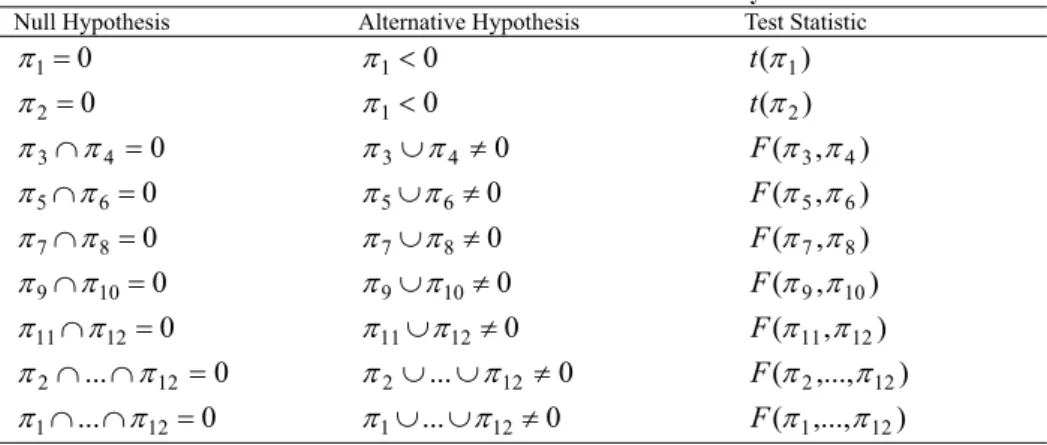
and for π_{1 = L}= π₁₂ = 0 (F(π₁,...,π₁₂)). This paper uses the critical values tabulated by Franses and Hobijn (1997) for each test. These tests for unit roots are summarized in Table 1.

Table 1. Tests of Seasonal Unit Root in Monthly Data

Null Hypothesis Alternative Hypothesis Test Statistic

0 1= π π1<0 t(π1) 0 2= π π₁<0 t(π₂) 0 4 3∩π = π π3∪π4 ≠0 F(π3,π4) 0 6 5∩π = π π₅∪π₆≠0 F(π₅,π₆) 0 8 7∩π = π π7∪π8≠0 F(π7,π8) 0 10 9∩π = π π₉∪π₁₀≠0 F(π₉,π₁₀) 0 12 11∩π = π π11∪π12≠0 F(π11,π12) 0 ... ₁₂ 2∩ ∩π = π π₂∪...∪π₁₂≠0 F(π₂,...,π₁₂) 0 ... 12 1∩ ∩π = π π1∪...∪π12≠0 F(π1,...,π12)

There are some other types of test for seasonal unit roots. Some examples are Canova and Hansen (1995), Caner (1998), Taylor and Leybourne (1999), and Shin and So (2000). However, the most useful point of the HEGY type test is its simplic-ity. We just run ordinary least squares on equation (9) and test each unit root using the t-value or F-value and appropriate critical values. As is discussed by Taylor and Leybourne (1999), other tests are just complements to the established HEGY type test.

3. Data and Empirical Results

Data: The Morgan Stanley Capital International Index (MSCI Index) is used as the stock price index of the G7 countries. Monthly data from December 1969 to March 2001 are analyzed. Each index shows the end-of-month value and is expressed as a logarithm.

Seasonal Integration Tests: The seasonal integration test was conducted based on equation (9). For the deterministic part of equation (9), two lines of analysis were used to examine the robustness of the result. The first considered both the seasonal dummy and the time trend, whereas the second considered only the seasonal dummy. The lag order p in equation (9) was selected using the Schwarz Bayesian Informa-tion Criterion (SBIC). To determine the value of lag order p, values from 0 to 6 were tried, and that giving the lowest SBIC was selected. Consequently, p=0 was se-lected for the index in all countries, proving that there was no need for the aug-mented terms in equation (9).

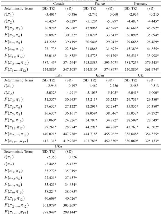
Table 2. Results of Seasonal Integration Tests

Canada France Germany

Deterministic Terms (SD, TR) (SD) (SD, TR) (SD) (SD, TR) (SD) ) (π₁ t -3.401* -0.386 -2.747 0.060 -2.934 -0.215 ) (π2 t -6.424* -6.329* -5.120* -5.089* -4.483* -4.445* ) , (π₃ π₄ F 36.928* 36.060* 42.996* 42.678* 46.668* 45.692* ) , (π5π6 F 30.892* 30.032* 33.829* 33.643* 36.099* 35.694* ) , (π₇ π₈ F 41.228* 39.419* 30.540* 29.945* 29.668* 28.469* ) , (π9 π10 F 23.173* 22.518* 31.886* 31.697* 45.389* 44.855* ) , (π₁₁π₁₂ F 36.016* 34.838* 44.572* 44.179* 36.531* 35.998* ) ,..., (π2 π12 F 387.145* 374.764* 393.858* 393.507* 381.723* 376.543* ) ,..., (π₁ π₁₂ F 354.886* 347.308* 364.810* 374.897* 350.880* 361.974* Italy Japan UK Deterministic Terms (SD, TR) (SD) (SD, TR) (SD) (SD, TR) (SD) ) (π₁ t -2.946 -0.497 -1.462 -2.256 -2.483 -0.513 ) (π₂ t -5.032* -4.991* -5.105* -5.105* -6.041* -6.000* ) , (π₃ π₄ F 31.357* 30.963* 33.211* 33.232* 29.731* 29.380* ) , (π₅π₆ F 27.632* 27.122* 32.291* 32.284* 35.855* 35.380* ) , (π₇ π₈ F 36.637* 36.101* 38.059* 38.046* 35.053* 34.292* ) , (π₉ π₁₀ F 25.060* 24.826* 34.787* 34.772* 28.509* 28.549* ) , (π₁₁π₁₂ F 29.261* 28.974* 44.291* 44.288* 43.767* 43.502* ) ,..., (π₂ π₁₂ F 440.021* 447.738* 444.718* 455.962* 358.648* 354.555* ) ,..., (π₁ π₁₂ F 412.131* 419.928* 407.789* 452.330* 330.060* 325.133* USA Deterministic Terms (SD, TR) (SD) ) (π₁ t -2.353 0.526 ) (π₂ t -5.445* -5.432* ) , (π₃ π₄ F 35.272* 35.019* ) , (π₅π₆ F 27.421* 27.457* ) , (π₇ π₈ F 35.421* 34.634* ) , (π₉ π₁₀ F 38.224* 38.085* ) , (π₁₁π₁₂ F 40.609* 40.626* ) ,..., (π₂ π₁₂ F 301.979* 303.209* ) ,..., (π₁ π₁₂ F 278.949* 299.144*

(SD, TR) shows that the estimation equations include twelve seasonal dummies and a time trend. (SD) shows that the estimation equations include twelve seasonal dummies.

Table 2 show the empirical results from each country’s data. These tables raise some interesting points. First, they make it clear that the nonseasonal unit root can-not be rejected for all countries. In Japan, for instance, as Table 2 shows, t(π₁) is –1.462 when the seasonal dummy and the time trend are used as deterministic terms, and t(π₁) is –2.256 when the time trend is excluded. In neither case is it possible to reject the existence of nonseasonal unit roots. This result is common to all countries except Canada, as is clearly shown in Table 2. In Canada, the null hy-pothesis of a nonseasonal unit root is rejected when the seasonal dummy and the time trend are used as deterministic terms, but not when only the seasonal dummy is used as a deterministic term. Secondly, the tables also show that the existence of seasonal unit roots should be rejected. In the case of Japan, shown in Table 2, the null hypothesis is rejected in all test statistics, from t(π₂) to F(π₁,...,π₁₂). Simi-lar results are obtained for other countries. Thus, stock prices do not have seasonal unit roots, and the (1−B) filter is effective.

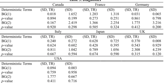
Table 3 shows the diagnostics of the empirical results. Each table shows the Breusch-Godfrey Lagrange multiplier test statistic for serial correlation in errors. In the Breusch-Godfrey test, the null hypothesis is that there is no serial correlation up to order q in the residuals. The Breusch-Godfrey statistic is computed as the number of observations times R2 from the regression. This statistic is asymptotically dis-tributed as χ2(q). As is clear from each table, no serial correlation was found from the residuals in any country. For the case of Japan, Table 3 shows the test statistics (p-value) 0.628 (0.428) to test the first-order serial correlation and 0.789 (0.674) to test the second-order serial correlation when the deterministic term includes the time trend and seasonal dummy. Similar results can be found for other countries. These show that the specification of the model used in Table 2 is appropriate.

Table 3. Diagnostics

Canada France Germany

Deterministic Terms (SD, TR) (SD) (SD, TR) (SD) (SD, TR) (SD) BG(1) 0.018 1.652 1.203 1.318 0.031 0.065 p-value 0.894 0.199 0.273 0.251 0.861 0.798 BG(2) 0.167 2.419 1.366 2.254 1.775 3.216 p-value 0.920 0.298 0.505 0.324 0.412 0.200 Italy Japan UK Deterministic Terms (SD, TR) (SD) (SD, TR) (SD) (SD, TR) (SD) BG(1) 0.240 0.272 0.628 0.725 0.370 0.008 p-value 0.624 0.602 0.428 0.395 0.543 0.929 BG(2) 0.811 1.042 0.789 1.056 2.308 4.239 p-value 0.667 0.594 0.674 0.590 0.315 0.120 USA Deterministic Terms (SD, TR) (SD) BG(1) 0.094 0.003 p-value 0.759 0.958 BG(2) 1.777 0.667 p-value 0.411 0.716

(SD, TR) shows that the estimation equations include twelve seasonal dummies and a time trend. (SD) shows that the estimation equations include twelve seasonal dummies.

BG(1) is the Breusch-Godfrey test statistic for first-order autocorrelation in the residuals. BG(2) is the Breusch-Godfrey test statistic for second-order autocorrelation in the residuals.

4. Concluding Remarks

This paper performs seasonal integration tests based on stock price indices for G7 countries. If seasonality in stock prices is deterministic, it is possible to forecast the seasonal pattern, and thus investors can profit from this information. On the other hand, if seasonality in stock prices is stochastic, it is not possible to forecast the seasonal pattern, which is consistent with the hypothesis of market efficiency. Our results show that only nonseasonal unit roots were evident in all countries. Thus, it is clear that use of the (1−B) filter ensures the stationarity of stock prices, and the adoption of dummy variables is sufficient to deal with the seasonality of stock prices. The observed seasonality in stock prices is found to be deterministic, and thus it is possible to forecast seasonal patterns.

References

Ariel, R. A., (1987), “Monthly Effect in Stock Returns,” Journal of Financial

Eco-nomics, 18, 164-174.

Beaulieu, J. J. and J. A. Miron, (1993), “Seasonal Unit Root in Aggregate U.S. Data,” Journal of Econometrics, 55, 305-328.

Caner, M., (1998), “A Local Optimal Seasonal Unit Root Test,” Journal of Business

and Economic Statistics, 16, 349-359.

Canova, F. and B. E. Hansen, (1995), “Are Seasonal Pattern Constant over Time: A Test for Seasonal Stability,” Journal of Business and Economic Statistics, 13, 237-252.

Franses, P. H. and B. Hobijn, (1997), “Critical Values for Unit Root Tests in Sea-sonal Time Series,” Journal of Applied Statistics, 24, 25-47.

Ghysels, E., H. S. Lee, and J. Noh, (1994), “Testing for Unit Roots in Seasonal Time Series: Some Theoretical Extensions and a Monte Carlo Investigation,” Journal

of Econometrics, 62, 415-442.

Gultekin, M. N. and N. B. Gultekin, (1983), “Stock Market Seasonality: Interna-tional Evidence,” Journal of Financial Economics, 12, 469-481.

Hamori, S. and A. Tokihisa, (2000), “Seasonal Integration and Japanese Aggregate Data,” Applied Economics Letters, 7, 591-594.

Hylleberg, S., R. F. Engle, C. W. J. Granger, and B. S. Yoo, (1990), “Seasonal Inte-gration and CointeInte-gration,” Journal of Econometrics, 44, 215-238.

Hylleberg, S., C. Jorgensen, and N. K. Sorensen, (1993), “Seasonality in Macroeco-nomic Time Series,” Empirical EcoMacroeco-nomics, 18, 321-335.

Lakonishok, J. and S. Smidt, (1989), “Are Seasonal Anomalies Real? A Ninety-Year Perspectives,” Review of Financial Studies, 1, 403-425.

Lee, H. S. and P. L. Siklos, (1991), “Unit Roots and Seasonal Unit Roots in Macro-economic Time Series: Canadian Evidence,” Economics Letters, 35, 273-277. Peiro, A., (1994), “Daily Seasonality in Stock Returns: Further International

Evi-dence,” Economics Letters, 45, 227-232.

Cauchy Estimation and Recursive Mean Adjustments,” Journal of

Economet-rics, 99, 107-137.

Taylor, R. and S. Leybourne, (1999), “Detecting Seasonal Unit Roots: An Approach Based on the Sample Autocorrelation Function,” Manchester School, 67, 261-286.

Tokihisa, A. and S. Hamori, (2001), “Seasonal Integration for Daily Data,”

Econo-metric Reviews, 20, 187-200.

Wachtel, S. B., (1942), “Certain Observations on Seasonal Movement in Stock Prices,” Journal of Business, 15, 184-193.