Layer-Aware Design Partitioning for Vertical Interconnect Minimization
Abstract—Three-dimensional (3D) design technology, which
has potential to significantly improve design performance and ease heterogeneous system integration, has been extensively discussed in recent years. This emerging technology allows stacking multiple layers of dies and typically resolves the vertical inter-layer connection issue by through-silicon vias (TSVs). However, TSVs also occupy significant silicon estate as well as incur reliability problems. Therefore, the deployment of TSVs must be very judicious in 3D designs. In this paper, we propose an iterative layer-aware partitioning algorithm, named iLap, for TSV minimization in 3D structures. iLap iteratively applies multi-way min-cut partitioning to gradually divide a given design layer by layer in the bottom-up fashion. Meanwhile, iLap also properly fulfills a specific I/O pad constraint incurred by 3D structures to further improve its outcome. Experimental results show that iLap can reduce the number of TSVs by about 35% as compared to several existing state-of-the-art methods. We believe a good TSV-minimized 3D partitioning solution can serve as a good starting point for
further tradeoff operations between TSV count and wirelength.
Keywords- through-silicon via (TSV); 3D integration technology; layering; partitioning
I. INTRODUCTION
With the advance of semiconductor manufacturing process technology, ever-shrinking feature size and exponentially growing number of transistors on a single die are raising numerous tough challenges such as signal integrity, power integrity and dissipation, leakage power, clock distribution and yield issues [1]. In addition, the global interconnect delay fails to scale as the device delay does and is gradually dominating the system performance [1]. Therefore, a solution that can both alleviate the global interconnect delay bottleneck as well as provide new avenues to enable even advanced device and architecture innovations is eagerly demanded. While approaching the physical limitations, traditional scaling is no longer the best way for advancing manufacturing process technology, and hence three-dimensional (3D) technologies have been emerging in recent years [2]–[5]. 3D integrated circuit technologies enable stacking multiple dies on a single chip and provide several unique advantages compared to those conventional two-dimensional (2D) ones, such as higher system integration, better heterogeneous integration capability, and shorter global wirelength (i.e., better performance).
Among those state-of-the-art 3D integration technologies, through-silicon via (TSV) is one of the most promising methods to accomplish vertical interconnects between
different layers [4]. Fig. 1 illustrates a typical TSV-based 3D IC structure. By utilizing the wafer/die bonding techniques, TSVs cut across thinned silicon substrates to make inter-die connections, which results in high compatibility with the present typical CMOS processes. All external I/O signals must pass through those metal bumps located at the bottom of the 3D structure to bridge the internal logic and the external system. Nevertheless, compared with a typical 2D design, though a TSV-based 3D design can generally reduce the global interconnect delay, currently available TSV fabrication processes still suffer from relatively low yield as well as large TSV pitch size [6]. It is reported that in 22nm technology a TSV with 8μm pitch occupies roughly the same area as 1k SRAM cells (0.061μm2)[1], and TSV yield drops to about 80% in a 3D design with 2k TSVs [7]. Therefore, using less number of TSVs to complete a 3D design is highly desirable in terms of both yield and area cost. As a consequence, the issue of TSV minimization must be properly addressed in a design flow as stepping into the 3D IC era.
In general, 3D IC backend flows can be roughly classified into two categories. The first one is to combine TSV minimization into later design processes such as floorplanning [8] and placement [9][10], which aims at both objectives at the same time. However, the above mix-in-one problem is likely to become too complicated to be well handled. Alternatively, the authors in [11]–[13] all suggest that it is crucial to make 3D partitioning an independent stage in the backend flow as shown in Fig. 2. The suggested flow first partitions a given design into different layers and then solves the remaining problem by classical 2D techniques or their simple extensions. Hence, this methodology efficiently reduces the problem complexity while keeping the quality of results nearly at the same level [11][12]. Since the outcome of 3D partitioning mainly determines the number of required TSVs, several previous studies have been proposed to tackle the problem of 3D
Figure 1. A TSV-based 3D structure.
Ya-Shih Huang, Yang-Hsiang Liu, and Juinn-Dar Huang
Department of Electronics Engineering and Institute of ElectronicsNational Chiao Tung University, Hsinchu 30010, Taiwan {sali, ktysliu}@adar.ee.nctu.edu.tw, [email protected]
partitioning for TSV minimization. One solution is to solve the problem using integer linear programming (ILP) [14]. However, it can only solve small-size problem since its runtime grows exponentially as problem size increases. In [15][16], each of them develops a modified FM-based [17] partitioning method to obtain the resultant layer assignment. However, all these methods only focus on minimizing the total amount of TSVs or die area, and do nothing about evenly distributing TSVs among layers. Meanwhile, the authors of 3D FPGA synthesis frameworks TPR [18] and 3D MEANDER [19] alternatively use a two-step approach – first applying the well-known partitioning algorithm hMetis [20] to divide a design into a set of layer-unaware partitions, and then associating each partition with a layer (i.e., layer assignment) – to accomplish 3D design partitioning. Though hMetis is an efficient and effective multi-way min-cut partitioning tool, it lacks for the notion of layer. In general, a typical 2D partitioning algorithm basically gives a similar weight to a cut between any two partitions, whereas those weights can vary a lot in 3D partitioning and highly depend on whether two partitions (i.e., layers) are close or far away from each other.
Indeed, 3D designs can help minimize long interconnects through the extensive use of TSVs. However, utilizing too few TSVs may limit this benefit and even increase the total wirelength, while allocating too many TSVs surely enlarges design area size [6]. Though only focusing on TSV reduction cannot guarantee decrease of wirelength after placement and routing, a TSV-minimized (also area-minimized) partitioning technique should still be incorporated as a preprocessing stage in a 3D design flow, which provides a good starting point for further tradeoff between area and wirelength in the
following stages. Therefore, in this paper, we propose an iterative layer-aware partitioning algorithm, named iLap, which can both minimize the number of TSVs and smooth the distribution of TSVs in 3D structures. Unlike [15][16],
iLap is iterative and gradually produces the final result layer
by layer. Also unlike [18][19], which first perform layer-unaware partitioning then layering, iLap applies layer-aware partitioning at each iteration. Though iLap also utilizes hMetis as the kernel of its partitioning engine, the experiment results demonstrate that iLap can apparently do better TSV minimization than three other hMetis-based methods for various number of layers, and the required runtime is just few seconds. The rest of this paper is organized as follows. In Section II, we briefly introduce our motivations and the problem formulation. Section III details the proposed iterative layer-aware partitioning algorithm. The experimental results and analyses are reported in Section IV. Finally, the concluding remarks are given in Section V.
II. PROBLEM DESCRIPTION A. Motivation
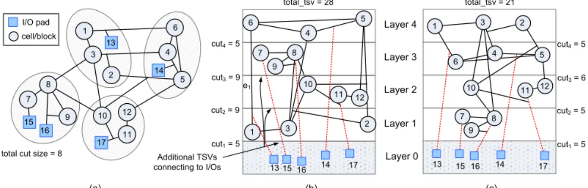
Fig. 3 demonstrates a simple 4-layer 3D partitioning example. A given design with its 4-way min-cut partitioning result is presented in Fig. 3(a). Based on the same initial partitioning result given in Fig. 3(a), Fig. 3(b) and 3(c) respectively illustrate the worst possible and the best possible 3D layering outcomes in terms of the number of TSVs. From the observations on Fig. 3, here we would like to highlight two key ideas.
Firstly, all external I/O terminals must be located in the bottom-most layer. It implies those square vertices representing I/O pads must always be located in Layer 0. As a result, extra TSVs are required to properly relocate those I/O pads. As shown in Fig. 3(b), five additional signal paths (in dotted lines) suggest that 13 more TSVs are further required. Those extra signal paths are generally unconsidered in conventional multi-way min-cut partitioning algorithms. It also explains why there is a big difference between the total cut size (=8) in Fig. 3(a) and the number of total TSVs (=28) in Fig. 3(b).
Secondly, different layer assignments usually result in different TSV requirements even the given initial partitioning result is identical. For instance, given the partitioning result shown in Fig. 3(a), the total number of
Layer 1 Layer 2 Layer 3 Layer 4 Layer 0 12 11 10 9 8 7 2 5 1 4 3 6 13 14 15 16 17 I/O pad cell/block 15 2 5 4 1 6 3 12 11 10 9 8 7 13 16 14 17 2 5 4 1 6 3 12 11 10 9 8 7 15 13 16 14 17 Additional TSVs connecting to I/Os cut4= 5 cut3= 9 cut2= 9 cut1= 5 cut4= 5 cut3= 6 cut2= 5 cut1= 5 (a) (b) (c)
total cut size = 8
total_tsv = 28 total_tsv = 21
e1
Figure 3. (a) A 4-way min-cut partitioned design,(b) the worst possible, and (c) the best possible 3D layering outcomes based on the partitioning in (a). Figure 2. Referenced backend flow for 3D ICs.
TSVs can range from 21 to 28 after examining all possible layer assignments. Nevertheless, the best layering result with the minimum number of TSVs shown in Fig. 4(d) cannot be derived from the initial partitioning outcome shown in Fig. 3(a), which is obtained from hMetis.
According to the aforementioned discussions, it should be evident that conventional multi-way min-cut partitioning algorithms virtually have no chances to perform 3D partitioning well in their original forms due to their unawareness about the fundamentals of vertical die-stacking structure. Therefore, a layer-aware partitioning algorithm specifically dedicated to 3D structures is strongly demanded for advanced 3D IC design methodologies.
B. Problem Formulation
A design is modeled as a hypergraph G = (V, E), where V is a set of vertices including a set of functional cells (or blocks) C and a set of I/O pads I (i.e., V = C ∪ I, C ∩ I = ); and E is a set of hyperedges. For each vertex v V, area(v) denotes the area cost of v. Each hyperedge is a subset of V, i.e., e V e E. A k-layer disjoint partition set of G with all the I/O terminals residing in the bottom-most layer is represented as L = {L0=I, L1, L2 … Lk}, where Li is the partition assigned to the i-th layer and is a subset of C; i.e., Li C 1 i k; Li ∩ Lj = i j, 1 i, j k; and L1 ∪ L2 ∪…∪Lk = C.
For a vertex v, layer(v) indicates which layer v actually resides in. That is, layer(v) = i, v Li. The range pair of a hyperedge e is defined as rp(e) = (b, t) if e connects vertices from the lower b-th layer to the upper t-th layer; i.e., v e,
b layer(v) t. Then the number of TSVs required to complete e can be calculated as tsv(e) = t – b. The layer
junction jcti is defined as the junction between the two
adjacent layers Li–1 and Li, 1 i k. The number of TSVs passing through jcti is further defined as cuti. Hence, the total number of TSVs, total_tsv, needed for a 3D partitioning solution L can be determined either by summing the required TSVs for all hyperedges (∑∈ ) or by summing TSVs passing through all junctions ( ∑ ). Consider the example shown in Fig. 3(b), rp(e1) = (1, 4) and thus tsv(e1) = 3. Similarly, the total number of TSVs in Fig. 3(b) is
total_tsv = ∑ = 5 + 9 + 9 + 5 = 28, including 15 TSVs
connecting between cells, and 13 TSVs connecting cells and I/O pads. We would like to emphasize again that classical partitioning algorithms usually have no idea about the I/O pad connection constraint and always underestimate the real TSV demand even excluding those TSVs for connecting cells and I/O pads (8 vs. 15 in the case shown in Fig. 3(a) and 3(b)) due to their layer-unawareness. Those are the major reasons why the classical min-cut-based partitioning solutions are generally not well optimized in 3D cases (shown later).
In this paper, we model the 3D partitioning problem as a layer-aware multi-way partitioning problem. Given a target 3D structure consisting of k layers stacking vertically, a design G, and the I/O pad constraint, our proposed algorithm partitions G into k sub-designs and each sub-design is explicitly associated with a vertical layer so that the total
number of TSVs is minimized. That is, given G = (V = C ∪
I, E) with layer(v) = 0 v I, our algorithm directly finds
the mapping, 1 layer(v) k v C, such that total_tsv is minimized.
III. PROPOSED ALGORITHM
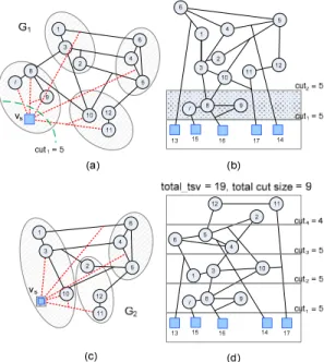
Here we propose our iterative partitioning framework that gradually constructs the solution from the bottom-most layer all the way to the topmost one. Consider that all I/O pads must reside in L0 by definition and then the number of TSVs through jct1 (i.e., cut1,) is always fixed to |I| no matter how other cells (or L1~Lk) get partitioned eventually. As a result, if we define G1 by compacting all the I/O pads into a supervertex vs and keeping all the connected hyperedges unchanged as shown in Fig. 4(a), it is evident that jct1 and
cut1 should still remain unchanged in G1. Next, an arbitrary conventional k-way area-balanced min-cut partitioning algorithm is applied on G1 to get k partitions, where area(vs) is set to zero to avoid disturbing area balancing during partitioning. Among those k disjoint partitions, exactly one partition ps can contain vs, which further suggests that the cells residing in ps should be located as close to the I/O pads as possible for cut minimization and thus should be assigned to L1. For example, the four dashed circles in Fig. 4(a) indicate the 4-way area-balanced min-cut partitioning result, and hence L1 is ultimately set to {7, 8, 9} as Fig. 4(b) depicts. Similarly, once the elements of L1 are determined, cut2 is therefore fixed. The next task then becomes how to decide which vertices should reside in L2. Again, since L0 and L1 are fixed at this point, jct2 and cut2 are both fixed no matter how other remaining cells (or L2~Lk) get partitioned later. As one can easily discover that the situation here is very similar to that of identifying L1 previously. Hence, if we further derive
G2 from G1 by compacting L1 into vs and apply (k–1)-way
Figure 4. (a) Compact I/O pads into vs then apply 4-way partitioning,
(b) assign {7, 8 ,9} to L1, (c) compact L1 into vs then apply 3-way
min-cut partitioning on G2, L2 can then be identified in the same fashion (as shown in Fig. 4(c)). That is, at each iteration our proposed algorithm always derives Gn+1 from Gn by further compacting Ln into vs, then applies (k–n)-way area-balanced min-cut partitioning to get Ln+1. This iterative process is not terminated until Lk–1 is identified. Fig. 4(d) illustrates the final result generated by the proposed algorithm, and the total TSV count is merely 19, which is smaller than those in Fig. 3(b) and 3(c) (28 and 21, respectively).
The proposed framework possesses following four unique features:
It invokes multi-way min-cut partitioning at every iteration. The major reason is to find the set of cells closest to the previously identified junctions, which potentially minimizes the TSVs of the current junction. To better mimic the final solution, min-cut partitioning helps distribute TSVs more evenly among all layers and hence potentially results in a more stable outcome.
Once a junction (and thus a cut) is fixed at some iteration, it is never altered at the following iterations. This ensures that good decisions made previously are never overthrown later.
At each iteration, only one partition is accepted and decisions for other partitions are actually discarded. Later, the updated graph topology is reexamined and better decisions are thus dynamically reacquired at the following iterations. For instance, L2 = {1, 3, 10} in Fig. 4(d) is not identical to any partition shown in Fig. 4(a). As a consequence, applying any one of conventional multi-way min-cut partitioning algorithms just once cannot get this kind of result. From the traditional partitioning perspective, the
result in Fig. 4(d) has a larger total cut size than the result given in Fig. 3(a) (9 vs. 8). However, we already show that the former one is actually a better 3D partitioning solution. Hence, it is obvious that the total cut size, which is layer-unaware, is apparently not an appropriate metric in 3D partitioning. Again, this is another evidence that classical multi-way min-cut partitioning algorithms can hardly compete with the proposed iterative framework.
In this work, we adopt the well-known hMetis as the internal partitioning engine since it is one of the best partitioning engines we can find today. However, our proposed framework can obviously co-work with any multi-way min-cut partitioning engines. It implies that a better engine (if any) may be adopted for better 3D partitioning results in the future.
The pseudo code of the complete algorithm is given in Fig. 5. All I/O pads are first compacted into a supervertex vs during initialization. Each iteration starts with (k–n+1)-way min-cut partitioning. Once partitioning is done, the vertices residing in the partition where vs is present are assigned to the current layer, i.e., Layer n. The number n always increases by one at every iteration end. At the final iteration, where n = k–1, the elements of Layer k–1 are identified after 2-way partitioning. Finally, the remaining cells are then automatically assigned to the topmost Layer k and the algorithm ends. That is, exact k–1 invocations of multi-way min-cut partitioning are required for getting one k-layer 3D partitioning result here.
IV. EXPERIMRNTS A. Environmental Setup
iLap has been implemented in C++/Linux environment.
We demonstrate the effectiveness of iLap through a series of comparisons with three hMetis-based methods: 1) hMetis: partitions are further layered according to their original sequential tags (i.e., in random order basically); 2)
EX-hMetis: partitions are best layered through exhaustively
examining all possible layer permutations; 3) EV-matrix: partitions are layered by the method described in [18]. Note that the three hMetis-based methods all start with the same set of partitions and thus the variances among their final results solely come from different layer assignments. We evaluate the performance of iLap and other three methods over a set of 14 test cases, consisting of 10 cases from the MCNC benchmark set [21], three large cases (cfft, aqua, and
video) from Altera [22], and one in-house 128-point FFT
design (fft128). They are intended to mimic complicated system designs integrating a large number of functional blocks. The number of blocks ranges from 1,047 to 53,491. Since the test cases selected in our experiments are all far larger than those used in [14], comparisons between iLap and the ILP-based approach proposed in [14] are therefore omitted in this paper. We perform ten experiment runs on every test case with different random seeds and take the average as the final result.
B. Results and Analyses
A set of experiments are conducted with various number of layers ranging from two to ten. Table I reports the TSV demands as the number of layers is set to 4. It seems
EV-matrix just performs equally well as plain hMetis.
Meanwhile, given a set of 4 partitions generated by hMetis,
EX-hMetis always picks the one with the lowest TSV count
out of 4! = 24 different layer permutations and consequently
EX-hMetis on average attains 16% TSV reduction as
compared with hMetis. Nevertheless, iLap can reduce TSV Initialization
1 n ← 1;
2 compact all I/O pads into a supervertex vs;
3 C ← C ∪ {vs}; Constructive Loop 4 while(n < k)
5 (k–n+1)-way min-cut partition(C); 6 foreach vi C – {vs} do 7 if part(vi) == part(vs) do 8 assign vi to Layer n; 9 C ← C – {vi}; 10 compact vi into vs; 11 n ←n + 1; 12 foreach vj C – {vs} do 13 assign vj to Layer k;
count by 36% and 24% on average as compared to hMetis and EX-hMetis, respectively. Moreover, for the largest three test cases (cfft, aqua, and video), iLap even outperforms
hMetis by more than 75%. Though hMetis is an excellent
multi-way min-cut partitioning algorithm, unfortunately it fails to be a good 3D partitioner due to its layer-unawareness. Even EX-hMetis, with exhaustive layer permutations, still cannot defeat iLap. Therefore, it concludes that a dedicated layer-aware 3D partitioning algorithm, like iLap, should be regarded as one of the essential components while constructing a sophisticated 3D IC design environment.
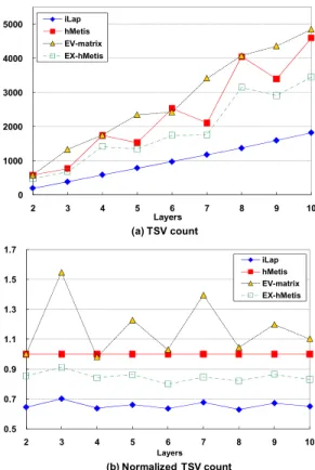
Next, Fig. 6(a) depicts the average TSV count over 14 test cases as a function of the number of layers; and three points are worth pointing out. Firstly, the more layers a design gets partitioned into, the more TSVs it generally requires. Secondly, iLap is the all-time winner from 2 layers to 10 layers among four methods. Thirdly, unlike the other three methods, the number of TSVs required by iLap raises very smoothly as the number of layers increases. Taking
hMetis as the baseline, Fig. 6(b) reveals the average ratios of
TSV count over the number of layers; and two points are worth mentioning here. Firstly, iLap constantly and steadily outperforms hMetis by about 35% in TSV count regardless of the number of layers. Secondly, EX-hMetis always outperforms hMetis, as expected.
Meanwhile, Fig. 7(a) presents the average standard deviations of TSV count over a different number of layers. Through constructing its outcome layer by layer, iLap can better balance the TSV count among junctions. From Fig. 7(a), it is evident that the standard deviation of TSV count associated with iLap is far better than those of the other three. As previously mentioned, a TSV occupies significant silicon estate so that high standard deviation of TSV count potentially worsens area imbalance among individual layers and even lowers the yield of a design. Fig. 7(b) reports the average maximum TSV count at some junction of a design over a different number of layers; and iLap always possesses the lowest values regardless of the number of layers. In other
words, a lower TSV count implies a smaller total area (including TSV area) after partitioning, and a smaller standard deviation of TSV count results in a more area-balanced partitioning outcome. The above two facts suggest that iLap tends to generate a smaller overall footprint of a 3D chip implementation. From another perspective, for some 3D logic structures, like 3D FPGAs, the number of pre-fabricated inter-layer TSVs is fixed. Hence a design mapping attempt is considered a failure as long as the required TSVs exceed the available ones only at one junction; and a high maximum TSV count definitely increases such chances. Lower maximum TSV count is considered a big plus especially in design flows for 3D regular logic structures such as 3D FPGAs.
Regarding the runtime efficiency issue, Fig. 7(c) gives the average runtime of 14 test cases in second over a different number of layers. It is evident that both hMetis and
EV-matrix are very time-efficient. The runtime required by iLap grows linearly as the number of layers increases. It is
mainly because the number of invocations for multi-way partitioning inside iLap also grows linearly as the number of layers increases. However, given the tremendous performance in TSV minimization, the time complexity of
iLap should be acceptable. For example, it only takes about
fifty seconds for iLap to partition the largest test case video into ten layers. As for EX-hMetis, since it has to check all possible layer permutations to find out the best one, the required runtime is thus exponential to the number of layers. Even if EX-hMetis can be further improved (e.g., by pruning) so that not all permutations need to be examined, the
TABLEI. TOTAL NUMBER OF TSVS WITH K =4
4 layers *Total TSVs Normalized to hMetis
Design iLap hMetis matrix EV- hMetis EX- iLap matrixEV- hMetis
EX-Tseng 304.2 356.3 361.2 346.1 0.85 1.01 0.97 Diffeq 244.9 344.5 351.0 270.3 0.71 1.02 0.78 Des 445.5 857.5 876.1 834.5 0.52 1.02 0.97 Bigkey 629.2 666.2 669.2 650.6 0.94 1.00 0.98 Frisc 655.2 714.1 719.0 688.7 0.92 1.01 0.96 elliptic 590.3 709.9 690.0 643.1 0.83 0.97 0.91 pdc 973.4 1049.5 1059.0 986.8 0.93 1.01 0.94 fft128 1313.9 1506.0 1524.8 1489.2 0.87 1.01 0.99 s38417 249.4 364.7 389.6 324.6 0.68 1.07 0.89 s38584.1 391.4 673.8 762.6 536.7 0.58 1.13 0.80 clma 491.4 721.2 654.6 496.5 0.68 0.91 0.69 cfft 244.4 999.2 480.3 338.5 0.24 0.48 0.34 aqua 909.6 7026.5 7167.4 4935.8 0.13 1.02 0.70 video 763.8 8370.7 8757.1 7255.0 0.09 1.05 0.87 Average - - - - 0.64 0.98 0.84
*The reported number is the average of 10 experiment runs. Figure 6. The number of required TSVs in different layers.
0 1000 2000 3000 4000 5000 2 3 4 5 6 7 8 9 10 Layers (a) TSV count iLap hMetis EV-matrix EX-hMetis 0.5 0.7 0.9 1.1 1.3 1.5 1.7 2 3 4 5 6 7 8 9 10 Layers (b) Normalized TSV count iLap hMetis EV-matrix EX-hMetis
improvement is limited to runtime efficiency only, while other TSV-related performance would still remain the same.
V. CONCLUSION
In this paper, we present an iterative layer-aware partitioning algorithm iLap targeting TSV minimization for 3D structures. It utilizes a multi-way min-cut partitioning engine inside its iterative framework to gradually construct the final solution layer by layer in the bottom-up fashion. The experimental results clearly demonstrate that iLap is capable of reducing total TSV count by about 35% compared to layer-unaware hMetis, experiencing a smoother TSV increase as the number of layers raises, distributing TSVs more evenly among different vertical layers, preventing any layer junction from having a burst number of TSVs, and only requires an acceptable runtime. Consequently, compared to the prior art, we believe iLap can generate a better TSV-minimized solution, which serves as a good starting point for further tradeoff between wirelength and number of TSVs in upcoming state-of-the-art 3D IC/FPGA design flows.
ACKNOWLEDGMENT
This work was supported in part by the National Science Council of Taiwan under Grant NSC 99-2220-E-009-037.
REFERENCES
[1] International Technology Roadmap for Semiconductor. Semiconductor Industry Association, 2009.
[2] K. Banerjee, S. J. Souri, P. Kapur, and K. C. Saraswat, “3-D ICs: a novel chip design for improving deep submicron interconnect performance and systems-on-chip integration,” Proc. IEEE, vol. 89, no. 5, pp. 602–633, 2001.
[3] A. W. Topol, D. C. La Tulipe, L. Shi, D. J. Frank, K. Bernstein, S. E. Steen, A. Kumar, G. U. Singco, A. M. Young, K. W. Guarini and M. Ieong, “Three-dimensional integrated circuits,” IBM J. of Research
and Development, vol. 50, no. 4/5, pp. 491–506, Jul./Sep. 2006.
[4] G. Philip, B. Christopher, and P. Ramm, Handbook of 3D integration. Wiley-VCH, 2008.
[5] C. Ferri, S. Reda, and R. I. Bahar, “Parametric yield management for 3D ICs: models and strategies for improvement,” J. Emerging
Technologies in Computing Systems, vol. 4, no. 4, Article ID 19, Oct.
2008.
[6] M. Pathak, Y.-J. Lee, T. Moon, and S. K. Lim, “Through-silicon via management during 3D physical design: when to add and how many?”
Proc. Int’l Conf. on Computed-Aided Design, pp. 387–394, 2010.
[7] A.-C. Hsieh, T. Hwang, M.-T. Chang, M.-H. Tsai, C.-M. Tseng and H.-C. Li, “TSV redundancy: architecture and design issues in 3D IC,”
Proc. Design, Automation & Test in Europe Conf. & Exibit., pp. 166–
171, 2010.
[8] Z. Li, X. Hong, Q. Zhou, S. Zeng, J. Bian, W. Yu, H. H. Yang, V. Pitchumani, and C.-K. Cheng, “Efficient thermal via planning approach and its application in 3-D floorplanning,” IEEE Trans. on
Computer-Aided Design of Integrated Circuits and Systems, vol. 26,
no. 4, pp. 645–658, Apr. 2007.
[9] B. Goplen and S. Sapatnekar, “Placement of 3D ICs with thermal and interlayer via considerations,” Proc. Design Automation Conf., pp. 626–631, 2007.
[10] J. Cong and G. Luo, “A multilevel analytical placement for 3D ICs,”
Proc. Asia and South Pacific Design Automation Conf., pp. 361–366,
2009.
[11] Z. Li, X. Hong, Q. Zhou, Y. Cai, J. Bian, H. H. Yang, V. Pitchumani, and C.-K. Cheng, “Hierarchical 3-D floorplanning algorithm for wirelenth optimization,” IEEE Trans. on Computer-Aided Design of
Integrated Circuits and Systems, vol. 53, no. 12, pp. 2637–2646, Dec.
2006.
[12] V. F. Pavlidis and E. G. Friedman, “Interconnect-based design methodology for three-dimensional integrated circuits,” Proc. IEEE, vol. 97, no. 1, pp. 123–140, Jan. 2009.
[13] C. Chiang and S. Sinha, “The road to 3D EDA tool deadiness,” Proc.
Asia and South Pacific Design Automation Conf., pp. 429–436, 2009.
[14] I. H.-R. Jiang, “Generic integer linear programming formulation for 3D IC partitioning,” 22nd IEEE Int’l SOC Conf., pp. 321–324, 2009. [15] D. H. Kim, K. Athikulwongse, and S. K. Lim, “A study of
through-silicon-via impact on the 3D stacked IC layout,” Proc. Int’l Conf. on
Computer-Aided Design, pp. 674–680, 2009.
[16] Y. C. Hu, Y. L. Chung, and M. C. Chi, “A multilevel multilayer partitioning algorithm for three dimensional integrated circuits,” Proc.
Int’l Symp. on Quality Electronic Design, pp. 483–487, 2010.
[17] C. M. Fiduccia and R. M. Mattheyses, “A linear time heuristic for improving network partitions,” Proc. Design Automation Conf., pp.175–181, 1982.
[18] C. Ababei, H. Mogal, and K. Bazargan, “Three-dimensional place and route for FPGAs,” IEEE Trans. on Computer-Aided Design of
Integrated Circuits and Systems, vol. 25, no. 6, pp. 1132–1140, Jun.
2006.
[19] K. Siozios, A. Bartzas, and D. Soudirs, “Architecture-level exploration of alternative interconnection schemes targeting to 3D FPGAs: a software-supported methodology,” Int’l J. of
Reconfigurable Computing, vol. 2008, Article ID 764942, 2008.
[20] G. Karypis, R. Aggarwal, V. Kumar, and S. Shekhar, “Multilevel hypergraph partitioning: applications in VLSI domain,” IEEE Trans.
on VLSI Systems, vol. 7, no. 1, pp. 69–79, Mar. 1999.
[21] S. Yang, “Logic synthesis and optimization benchmarks user guide,” Technical Report 1991-IWLS-UG-Saeyang, Microelectronics Center of North Carolina, 1991.
[22] http://www.eecs.berkeley.edu/~alanmi/benchmarks/altera/old/altera12 _blif_baf.zip.
Figure 7. More statistics from the experiments. 0 50 100 150 200 250 300 3 4 5 6 7 8 9 10 Layers
(a) Standard deviation of TSV count
iLap hMetis EV-matrix EX-hMetis 0 100 200 300 400 500 600 700 800 900 1000 2 3 4 5 6 7 8 9 10 Layers (b) Maximum TSV count iLap hMetis EV-matrix EX-hMetis 0 500 1000 1500 2000 2500 3000 3500 2 3 4 5 6 7 8 9 10 Layers (c) Runtime (seconds) iLap hMetis EV-matrix EX-hMetis 0 2 4 6 8 10 12 2 3 4 5 6 7 8 9 10