漲跌停板限制下的股價行為之研究

行政院國家科學委員會補助專題研究計畫成果

報告

※※※※※※※※※※※※※※※※※※※※※※※

※ 漲跌停板限制下的股價行為之研究 ※

※

Dynamics of Stock Return Under Price Limits ※

※※※※※※※※※※※※※※※※※※※※※※※

計畫類別： ˇ個別型計畫 □整合型計畫

計畫編號：NSC 89－2416－H－004－068

執行期間：八十九年八月一日至九十年十月三十一日

計畫主持人：郭維裕

本成果報告包括以下應繳交之附件：

□赴國外出差或研習心得報告一份

□赴大陸地區出差或研習心得報告一份

□出席國際學術會議心得報告及發表之論文各一份

□國際合作研究計畫國外研究報告書一份

執行單位：國立政治大學國際貿易學系

中

華

民 國 九十一 年 一 月 三十一 日

行政院國家科學委員會專題研究計畫成果報告

計畫編號：NSC 89-2416-H-004-006

執行期限：89 年 8 月 1 日至 90 年 10 月 31 日

主持人：郭維裕

執行機構及單位名稱：國立政治大學國際貿易學系

Abstr act

We examine the short-run dynamics among the autocorrelations of short-horizon stock returns, volatilities, and trading volumes. Using the volatility measure of Schwert (1989), we find results that are consistent with those of Campbell, Grossman, and Wang (1993) but contrary to those of Sentana and Wadhwani (1992) without taking the effects of price limits into account. In particular, based on the sample stocks, we find that the first-order autocorrelations of stock returns are generally negatively related to trading volumes whereas they are positively related to the volatilities of stock returns. Moreover, there does not exist significant relationship between the first-order autocorrelations of stock returns and the squares of trading volumes. These results imply that, opposed to what Sentana and Wadhwani (1992) have found, investors in Taiwan stock market follow negative feedback trading strategy. However, the results turn to quite different once the effects of price limits are taken into account. We find that although the trading volumes still have negative impact to the autocorrelations of stock returns, the volatility of stock returns exerts negative influence on the autocorrelations of stock returns as well. This result is consistent with that of Sentana and Wadhwani (1992) indicating that investors in Taiwan stock market actually adopt positive feedback trading strategy during the period of normal market condition while they become contrarian during the period of volatile market condition, i.e., hitting price limits. We also provide some indirect evidence that support the volatility spillover hypothesis, the delayed price discovery hypothesis, and the trading interference hypothesis about the effectiveness of price limit proposed and empirically tested by Kim and Rhee (1994).

Introduction

A large research body of stock return predictability reveals that stock returns are predictable at least in the short term. In addition to their own serial correlations, the predictability of stock returns can be exploited by using trading volume and stock return volatility as conditional variables. Campbell, Grossmand, and Wang (1993), Blume, Easley, and O’Hara (1994), Conrad, Hameed, and Niden (1994), Chordia and Swaminathan (2000), and Säfvenblad (2000) document that there exists a significant relation between the first-order autocorrelation of stock returns and the trading volumes. Stock prices tend to maintain their previous movements when the trading volumes are low whereas they incline to reverse more frequently when the trading volumes are high. In other words, the trading volume has a negative impact on the autocorrelation of short-horizon stock returns.

LeBaron (1992), Sentana and Wadhwani (1992), and Koutmos (1997) show that the volatility of stock price is another important determinant of the autocorrelations of stock returns. LeBaron (1992) find that the relation between the volatility of stock prices and the autocorrelation of stock returns is nonlinear. Sentana and Wadhwani (1992) construct a model to show that such relation actually depends on the trading strategy adopted by the investors in the stock market. If the investors follow a positive feedback trading strategy, then we expect to find a negative relationship between the volatility of stock prices and the first-order autocorrelation of stock returns. By contrast, this relation will become a positive one if the investors follow a negative feedback trading strategy. Koutmos (1997) presents strong evidence that positive feedback trading induces negative autocorrelation in index stock returns in Australia, Belgium, Germany, Italy, Japan, and UK stock markets. Although the evidence shows that the negative relation between the volatility of stock price and the first-order autocorrelation of stock return is significant and pervasive, these studies do

not take the influence of the trading volume into account when conducting their empirical tests. In view of the vast literature of the relation between the volatility of stock price and the trading volume, failing to consider this interlink between these two variables may result in biased results.

French and Roll (1986), Karpov (1987), Lamoureux and Lastrapes (1990), Lamoureux and Lastrapes (1994), Jones, Kaul, and Lipson (1994), Andersen (1996), and Bollerslev and Jubinski (1999) all document that there exists a positive causal relationship between the volatility of stock price and the trading volume. Sentana and Wadhwani (1992) also points out that the trading volume may be helpful in further clearing the interaction between the volatility of stock price and the first-order autocorrelation of stock returns. Therefore, it seems proper to jointly study the impact of the volatility of stock price and the trading volume on the predictability of short-horizon stock returns as Campbell, Grossman, and Wang (1993). This is the methodology we follow in this article.

This paper studies the short-term dynamic among stock returns, trading volume, and stock price volatility in Taiwan stock market. Such a study in Taiwan stock market is complicated by a special feature of the trading mechanism in the market: the price limit. As Kim and Rhee (1994) point out, the price limit causes the volatility of stock price to spillover to the next trading day, induces positive autocorrelations of stock returns by preventing stock prices from efficiently reaching their equilibrium levels, and damages market liquidity by forcing investors to wait until the next trading day to continue their transactions resulting in another spillover effect of trading volume. Due to the price limit of Taiwan stock market, the aforementioned results should be scrutinized by specifically taking the effects of price limit into account. This is the primary contribution of this paper. Although Shen and Wong (1998) has conducted a similar study, our paper is different from their in several ways. First, we

use a different sample period from but the same sample stocks as Shen and Wong (1998). We also employ a different measure of volatility suggested by Schwert (1989). Hence, our study may serve as a out-of-sample test of the results documented in Shen and Wong (1998). Second, we specifically incorporate the price limit into the dynamics among the autocorrelations of stock returns, the volatility of stock prices, and the trading volume. Specifically, we investigate the dynamics in three different regimes that are identified by the occurrence of a upper-limit hit, a lower-limit hit, and a null hit. If the price limit does exert significant influence to the aforementioned dynamics, we expect to find different relations in different regimes. Third, to check the robustness of our results, we also perform the same tests in two subperiods.

we find results that are consistent with those of Campbell, Grossman, and Wang (1993) but contrary to those of Sentana and Wadhwani (1992) without taking the effects of price limits into account. In particular, based on the sample stocks, we find that the first-order autocorrelations of stock returns are generally negatively related to trading volumes whereas they are positively related to the volatilities of stock returns. Moreover, there does not exist significant relationship between the first-order autocorrelations of stock returns and the squares of trading volumes. These results imply that, opposed to what Sentana and Wadhwani (1992) have found, investors in Taiwan stock market follow negative feedback trading strategy. However, the results turn to quite different once the effects of price limits are taken into account. We find that although the trading volumes still have negative impact to the autocorrelations of stock returns, the volatility of stock returns exerts negative influence on the autocorrelations of stock returns as well. This result is consistent with that of Sentana and Wadhwani (1992) indicating that investors in Taiwan stock market actually adopt positive feedback trading strategy during the period of normal

market condition while they become contrarian during the period of volatile market condition, i.e., hitting price limits. We also provide some indirect evidence that support the volatility spillover hypothesis, the delayed price discovery hypothesis, and the trading interference hypothesis about the effectiveness of price limit proposed and empirically tested by Kim and Rhee (1994).

We summarize main results of our paper in the following tables.

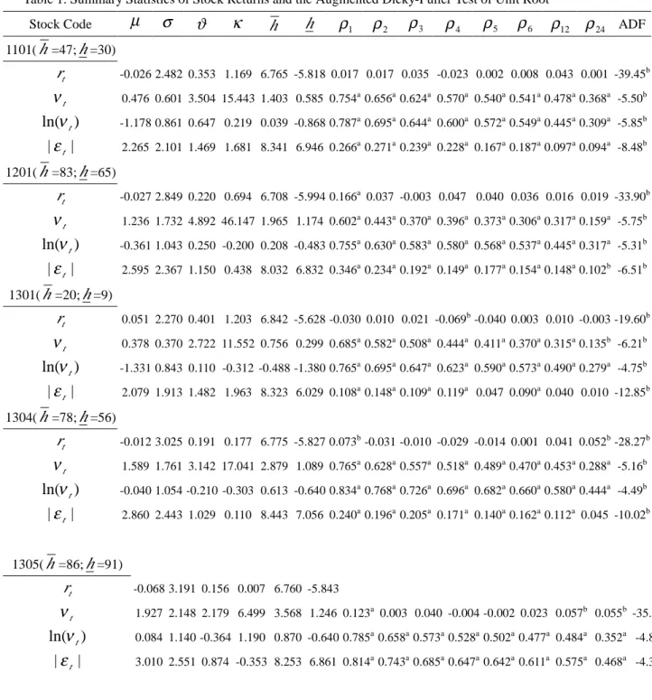
Table 1. Summary Statistics of Stock Returns and the Augmented Dicky-Fuller Test of Unit Root

Stock Code µ σ ϑ κ _h h ρ₁ ρ₂ ρ₃ ρ₄ ρ₅ ρ₆ ρ₁₂ ρ₂₄ ADF 1101(h=47;h=30) t r -0.026 2.482 0.353 1.169 6.765 -5.818 0.017 0.017 0.035 -0.023 0.002 0.008 0.043 0.001 -39.45b t ν 0.476 0.601 3.504 15.443 1.403 0.585 0.754a0.656a0.624a 0.570a 0.540a0.541a0.478a0.368a -5.50b ) ln(ν_t -1.178 0.861 0.647 0.219 0.039 -0.868 0.787a0.695a0.644a 0.600a 0.572a0.549a0.445a0.309a -5.85b | |ε_t 2.265 2.101 1.469 1.681 8.341 6.946 0.266a0.271a0.239a 0.228a 0.167a0.187a0.097a0.094a -8.48b 1201(h=83;h=65) t r -0.027 2.849 0.220 0.694 6.708 -5.994 0.166a 0.037 -0.003 0.047 0.040 0.036 0.016 0.019 -33.90b t ν 1.236 1.732 4.892 46.147 1.965 1.174 0.602a0.443a0.370a 0.396a 0.373a0.306a0.317a0.159a -5.75b ) ln(ν_t -0.361 1.043 0.250 -0.200 0.208 -0.483 0.755a0.630a0.583a 0.580a 0.568a0.537a0.445a0.317a -5.31b | |ε_t 2.595 2.367 1.150 0.438 8.032 6.832 0.346a0.234a0.192a 0.149a 0.177a0.154a0.148a0.102b -6.51b 1301(h=20;h=9) t r 0.051 2.270 0.401 1.203 6.842 -5.628 -0.030 0.010 0.021 -0.069b-0.040 0.003 0.010 -0.003 -19.60b t ν 0.378 0.370 2.722 11.552 0.756 0.299 0.685a0.582a0.508a 0.444a 0.411a0.370a0.315a0.135b -6.21b ) ln(ν_t -1.331 0.843 0.110 -0.312 -0.488 -1.380 0.765a0.695a0.647a 0.623a 0.590a0.573a0.490a0.279a -4.75b | |ε_t 2.079 1.913 1.482 1.963 8.323 6.029 0.108a0.148a0.109a 0.119a 0.047 0.090a 0.040 0.010 -12.85b 1304(h=78;h=56) t r -0.012 3.025 0.191 0.177 6.775 -5.827 0.073b-0.031 -0.010 -0.029 -0.014 0.001 0.041 0.052b-28.27b t ν 1.589 1.761 3.142 17.041 2.879 1.089 0.765a0.628a0.557a 0.518a 0.489a0.470a0.453a0.288a -5.16b ) ln(ν_t -0.040 1.054 -0.210 -0.303 0.613 -0.640 0.834a0.768a0.726a 0.696a 0.682a0.660a0.580a0.444a -4.49b | |ε_t 2.860 2.443 1.029 0.110 8.443 7.056 0.240a0.196a0.205a 0.171a 0.140a0.162a0.112a 0.045 -10.02b 1305(h=86;h=91) t r -0.068 3.191 0.156 0.007 6.760 -5.843 t ν 1.927 2.148 2.179 6.499 3.568 1.246 0.123a 0.003 0.040 -0.004 -0.002 0.023 0.057b 0.055b -35.63b ) ln(ν_t 0.084 1.140 -0.364 1.190 0.870 -0.640 0.785a0.658a0.573a0.528a0.502a0.477a 0.484a 0.352a -4.89b | |ε_t 3.010 2.551 0.874 -0.353 8.253 6.861 0.814a0.743a0.685a0.647a0.642a0.611a 0.575a 0.468a -4.34b

1402(h=62;h=45) 0.210a0.215a0.167a0.139a0.141a0.139a 0.145a 0.118a -6.99b t r 0.034 2.905 0.219 0.250 6.784 -5.841 t ν 0.534 0.474 2.156 6.326 1.127 0.460 0.061b0.035 0.018 -0.020 -0.014 -0.013 0.022 -0.052b-37.74b ) ln(ν_t -0.953 0.813 0.039 -0.389 -0.062 -1.174 0.709a0.602a0.532a0.478a0.436a0.424a 0.327a 0.178b -6.96b | |ε_t 2.747 2.364 1.004 0.087 8.312 6.563 0.743a0.675a0.613a0.579a0.550a0.528a 0.426a 0.235b -5.76b 1407(h=124;h=104) 0.197a0.145a0.194a0.166a0.154a0.165a 0.113a 0.092b -7.69b t r -0.113 3.341 0.200 -0.142 6.626 -5.868 t ν 1.130 1.286 2.469 7.837 1.316 0.762 0.180a_{-0.028 0.018 0.020 0.002 0.020 0.001 0.015 -21.77}b ) ln(ν_t -0.375 1.003 0.040 0.068 -0.225 -0.905 0.779a_0.681a_0.636a_0.593a_0.551a_0.538a _0.466a _0.395a _-4.75b | |ε_t 3.193 2.569 0.804 -0.444 8.023 6.617 0.812a_0.732a_0.701a_0.673a_0.652a_0.633a _0.553a _0.469a _-4.55b 1408(h=98;h=88) 0.307a_0.286a_0.242a_0.211a_0.223a_0.183a _0.172a _0.178a _-7.51b t r -0.107 3.107 0.203 0.187 6.614 -5.890 0.166a-0.029 0.006 0.050 0.022 0.042 -0.056b 0.000 -27.38b t ν 1.137 1.491 3.733 18.130 1.516 0.816 0.785a0.643a0.582a0.531a0.483a0.443a 0.318a 0.216a -7.18b ) ln(ν_t -0.359 0.947 0.257 0.341 -0.052 -0.670 0.799a0.699a0.659a0.624a0.604a0.592a 0.504a 0.401a -4.91b | |ε_t 2.888 2.507 0.963 -0.098 8.089 6.878 0.368a0.360a0.294a0.268a0.272a0.219a 0.237a 0.209a -5.91b 1433(h=43;h=24) t r 0.060 2.576 0.359 0.694 6.829 -5.641 0.012 -0.003 -0.026 -0.045 -0.025 0.029 -0.004 -0.013 -39.68b t ν 0.488 0.527 2.649 7.611 0.445 0.310 0.726a 0.606a 0.536a0.513a0.466a0.430a0.397a0.230a -5.68b ) ln(ν_t -1.168 0.955 0.056 -0.339 -0.173 -1.383 0.813a 0.730a 0.678a0.650a0.627a0.606a0.538a0.386a -4.67b | |ε_t 2.394 2.145 1.243 0.931 8.430 6.717 0.203a 0.179a 0.152a0.127a0.128a0.106a0.087a 0.016 -12.01b 1504(h=39;h=34) t r -0.005 2.525 0.254 0.758 6.763 -5.054 -0.015 -0.052b0.049 -0.028 -0.030 0.018 0.019 -0.004 -22.92b t ν 0.573 0.765 4.148 27.871 1.753 0.731 0.748a 0.676a 0.656a0.601a0.583a0.587a0.602a0.459a -3.56b ) ln(ν_t -1.037 0.921 0.471 0.116 0.200 -0.725 0.786a 0.713a 0.674a0.634a0.617a0.600a0.507a0.387a -4.61b | |ε_t 2.347 2.102 1.312 1.261 8.444 6.110 0.275a 0.262a 0.219a0.233a0.235a0.222a0.139a0.163a -9.12b 1602(h=60;h=44) t r 0.019 2.833 0.242 0.331 6.792 -5.754 0.032 0.000 0.010 -0.001 0.011 0.014 0.037 -0.001 -38.83b t ν 1.052 1.241 3.224 14.026 2.838 1.185 0.771a _0.667a _0.600a_0.536a_0.509a_0.501a_0.409a_0.279a _-5.13b ) ln(ν_t -0.398 0.923 0.242 -0.036 0.745 -0.394 0.796a _0.690a _0.630a_0.596a_0.578a_0.550a_0.460a_0.271a _-5.06b | |ε_t 2.685 2.278 1.125 0.489 8.398 6.971 0.235a _0.221a _0.188a_0.170a_0.145a_0.128a_0.105a_0.095b _-8.70b 1604(h=61;h=40) t r 0.003 2.663 0.356 0.874 6.791 -5.707 0.121a -0.002 0.011 -0.016 -0.044 0.000 0.026 -0.006 -35.45b t ν 0.438 0.676 4.379 25.957 0.822 0.186 0.720a 0.592a 0.565a0.495a0.450a0.465a0.366a0.239a -5.32b ) ln(ν_t -1.462 1.094 0.221 -0.039 -0.699 -2.030 0.825a 0.747a 0.717a0.694a0.679a0.657a0.566a0.454a -4.88b | |ε_t 2.456 2.208 1.311 1.066 8.296 6.712 0.277a 0.257a 0.235a0.167a0.156a0.201a0.176a0.165a -6.76b

1702(h=46;h=31) t r -0.026 2.611 0.220 0.701 6.727 -5.858 0.089a-0.034 -0.048 -0.037 0.032 0.040 -0.030 0.024 -23.94b t ν 0.546 0.751 3.382 15.517 1.363 0.463 0.746a0.552a0.488a 0.477a 0.441a0.406a0.333a0.250a -6.31b ) ln(ν_t -1.280 1.220 -0.320 0.932 -0.019 -1.609 0.825a0.756a0.711a 0.691a 0.651a0.638a0.578a0.495a -4.43b | |ε_t 2.428 2.138 1.262 0.982 8.055 7.104 0.265a0.200a0.165a 0.148a 0.118a0.147a0.114a0.097b -7.54b 1802(h=28;h=23) t r 0.014 2.219 0.338 1.478 6.815 -5.128 0.038 -0.033 -0.040 -0.080a _{0.035 0.003 0.018 0.050 -18.82}b t ν 0.234 0.276 2.791 9.978 0.574 0.338 0.716a_0.600a_0.548a _0.514a _0.496a_0.459a_0.424a_0.275a _-5.23b ) ln(ν_t -1.938 0.969 0.271 -0.438 -0.820 -1.437 0.757a_0.682a_0.629a _0.611a _0.605a_0.573a_0.511a_0.379a _-4.52b | |ε_t 1.996 1.899 1.565 2.313 8.320 5.971 0.274a_0.206a_0.178a _0.190a _0.168a_0.097a_0.136a_0.145a _-7.31b 1905(h=54;h=58) t r -0.023 2.914 0.118 0.217 6.757 -5.897 0.108a-0.036 -0.048 0.021 0.019 -0.017 -0.007 0.022 -23.95b t ν 1.507 1.513 2.228 6.529 3.266 1.204 0.712a0.579a0.533a 0.495a 0.422a0.442a0.405a0.281a -5.14b ) ln(ν_t -0.022 0.964 -0.183 -0.057 0.879 -0.181 0.799a0.717a0.662a 0.623a 0.589a0.580a0.537a0.438a -4.62b | |ε_t 2.750 2.339 1.006 0.127 8.283 6.960 0.254a0.185a0.180a 0.160a 0.094a0.105a0.110a0.066b -8.06b 1907(h=33;h=23) t r -0.026 2.414 0.238 1.018 6.975 -5.659 0.077a-0.041 -0.046 0.005 -0.022 0.001 -0.019 0.011 -24.23b t ν 0.182 0.227 3.369 15.971 0.649 0.265 0.751a0.608a0.557a 0.513a 0.454a0.412a0.402a0.261a -5.37b ) ln(ν_t -2.214 1.008 -0.047 1.118 -0.657 -2.029 0.796a0.709a0.661a 0.619a 0.587a0.552a0.459a0.317a -5.43b | |ε_t 2.200 2.033 1.374 1.497 8.091 6.566 0.313a0.220a0.204a 0.183a 0.134a0.142a0.104a0.095b -7.84b 2002(h=13;h=8) t r 0.022 1.811 0.649 2.401 6.801 -4.573 -0.043 -0.021 0.012 -0.026 0.005 0.005 0.010 -0.014 -41.81b t ν 0.356 0.375 2.969 11.386 1.239 0.302 0.737a0.604a0.560a 0.525a 0.482a0.459a0.366a0.265a -5.82b ) ln(ν_t -1.389 0.804 0.440 -0.048 0.040 -1.603 0.767a0.666a0.632a 0.605a 0.582a0.564a0.478a0.374a -5.01b | |ε_t 1.681 1.565 1.989 4.722 8.531 4.732 0.174a0.146a0.143a 0.084a 0.092a0.097a 0.026 0.038 -11.25b 2103(h=55;h=42) t r -0.056 2.782 0.300 0.559 6.761 -5.757 0.076a_{-0.044 0.005 -0.037 -0.018 0.016 -0.012 0.025 -12.19}b t ν 0.741 0.917 3.220 14.543 0.571 0.409 0.722a_0.596a_0.515a _0.466a _{0.450a 0.436}a_0.309a _{0.128 -6.46}b ) ln(ν_t -0.799 0.979 0.219 -0.141 -0.030 -1.170 0.811a_0.715a_0.663a _0.613a _0.585a_0.555a_0.476a_0.291a _-5.32b | |ε_t 2.574 2.311 1.156 0.468 8.351 6.799 0.342a_0.303a_0.237a _0.201a _0.193a_0.172a_0.172a_0.133a _-7.04b 2201(h=30;h=18) t r 0.050 2.452 0.236 0.809 6.822 -5.721 0.017 -0.038 0.039 -0.066b-0.004 -0.005 -0.007 -0.006 -21.13b t ν 0.461 0.457 2.287 7.223 0.390 0.279 0.681a0.586a0.554a 0.526a 0.492a0.456a0.352a0.244a -6.59b

) ln(ν_t -1.190 0.936 -0.090 -0.384 -0.213 -1.509 0.810a0.731a0.702a 0.686a 0.661a0.633a0.573a0.501a -4.32b | |ε_t 2.295 2.010 1.347 1.448 8.401 6.748 0.149a0.125a0.113a 0.084a 0.063b0.053b0.049 0.066b-10.06b 2301(h=65;h=73) t r 0.080 3.224 0.043 -0.184 6.792 -5.787 0.085a _{0.011 0.030 0.032 0.000 -0.017 0.013 0.007 -36.78}b t ν 2.846 2.658 1.833 4.586 4.108 2.261 0.757a_0.648a_0.601a _0.578a _0.552a_0.541a_0.516a_0.398a _-4.39b ) ln(ν_t 0.622 0.987 -0.502 1.105 1.091 0.016 0.791a_0.693a_0.664a _0.646a _0.621a_0.599a_0.524a_0.425a _-4.66b | |ε_t 3.141 2.484 0.799 -0.358 8.340 6.957 0.224a_0.180a_0.211a _0.224a _0.193a_0.169a_0.131a_0.100b _-6.55b 2501(h=51;h=21) t r -0.025 2.565 0.422 0.839 6.760 -5.253 -0.001 -0.051b-0.034 -0.058b 0.018 0.040 -0.047 0.012 -11.15b t ν 0.349 0.379 2.837 10.572 0.773 0.512 0.700a 0.574a 0.527a 0.445a 0.405a 0.389a0.332a0.255a -5.97b ) ln(ν_t -1.455 0.875 0.227 -0.005 -0.548 -1.160 0.755a 0.667a 0.638a 0.577a 0.550a 0.530a0.451a0.370a -4.79b | |ε_t 2.344 2.153 1.326 1.143 8.369 6.882 0.195a 0.198a 0.188a 0.164a 0.110a 0.139a 0.029 0.064b-10.06b 2704(h=38;h=28) t r -0.039 2.519 0.247 0.829 6.733 -5.436 0.011 -0.027 -0.043 -0.035 0.026 -0.017 -0.022 0.049 -13.71b t ν 1.075 1.613 4.124 28.357 2.206 0.560 0.732a 0.649a 0.559a 0.521a 0.483a 0.462a0.311a0.164b -6.47b ) ln(ν_t -0.700 1.303 -0.150 -0.217 0.240 -1.264 0.797a 0.709a 0.658a 0.642a 0.626a 0.608a0.542a0.444a -4.39b | |ε_t 2.316 2.125 1.297 1.132 8.419 6.516 0.253a 0.209a 0.182a 0.115a 0.103a 0.109a 0.023 0.042 -9.17b 2801(h=55;h=30) t r -0.043 2.549 0.454 1.117 6.763 -5.409 0.054b 0.000 0.017 -0.001 -0.032 0.023 0.008 -0.002 -37.92b t ν 0.496 0.461 2.470 8.265 1.126 0.538 0.653a 0.530a 0.446a 0.383a 0.350a 0.314a0.162a 0.032 -10.09b ) ln(ν_t -1.035 0.824 -0.044 0.123 -0.033 -0.786 0.730a 0.633a 0.568a 0.515a 0.475a 0.442a0.303a0.173b -8.15b | |ε_t 2.306 2.158 1.390 1.338 8.363 6.266 0.217a 0.200a 0.173a 0.141a 0.138a 0.080a0.070b0.052 -9.83b 2903(h=34;h=20) t r -0.020 2.411 0.306 1.012 6.766 -5.481 0.019 -0.017 0.059b _{-0.045 -0.067}b _{0.005 -0.037 0.020 -17.07}b t ν 0.414 0.584 4.973 37.105 1.318 0.438 0.699a _0.586a _0.480a _0.468a _0.438a _0.462a_0.303a_0.244a _-6.02b ) ln(ν_t -1.377 0.940 0.409 0.191 -0.079 -1.300 0.778a _0.680a _0.626a _0.583a _0.559a _0.541a_0.474a_0.363a _-4.93b | |ε_t 2.205 2.000 1.388 1.545 8.334 6.239 0.218a _0.224a _0.197a _0.122a _0.088a _0.152a_0.080b_0.099a _-9.95b µ, σ , ϑ, and κ are the mean, standard deviation, coefficient of skewness, and the coefficient of excess

kurtosis of stock returns, respectively. The asymptotic standard errors of the coefficient of skewness and the

coefficient of excess kurtosis are

N

6 _and

N

24 _{. In our case, the number of observations is 1626.}

Hence, the asymptotic standard errors of the coefficient of skewness and the coefficient of excess kurtosis are 0.0015 and 0.0030, respectively.

a_{, and} b _{mean that the serial correlations of stock returns are greater than their three and two asymptotic standard}

errors, respectively, and that the statistic of the Augmented Dicky-Fuller test of unit root is significant at 1% and 5% levels, respectively.

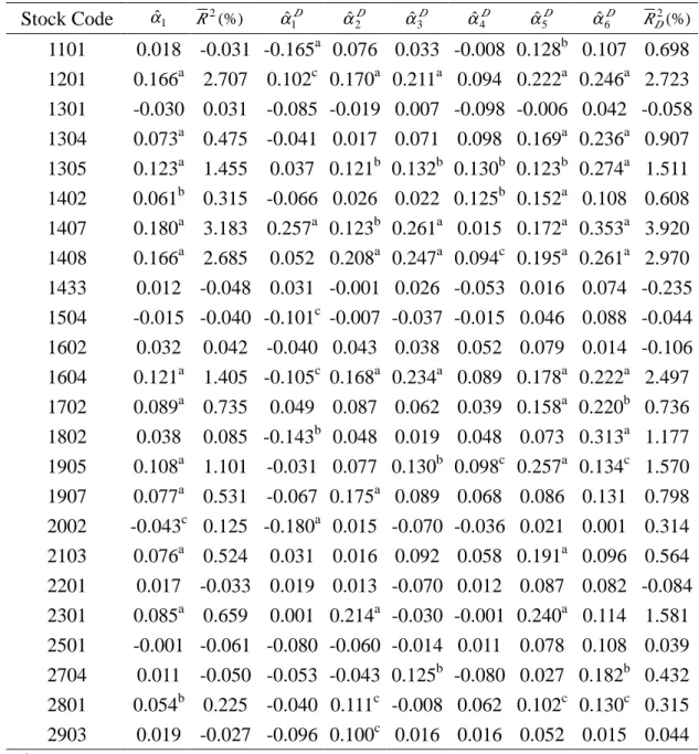
Table 2. The Estimated Benchmark Model Stock Code αˆ1 R2(%) αˆ1D D 2 ˆ α D 3 ˆ α D 4 ˆ α D 5 ˆ α D 6 ˆ α R_D2(%) 1101 0.018 -0.031 -0.165a 0.076 0.033 -0.008 0.128b 0.107 0.698 1201 0.166a 2.707 0.102c 0.170a 0.211a 0.094 0.222a 0.246a 2.723 1301 -0.030 0.031 -0.085 -0.019 0.007 -0.098 -0.006 0.042 -0.058 1304 0.073a 0.475 -0.041 0.017 0.071 0.098 0.169a 0.236a 0.907 1305 0.123a 1.455 0.037 0.121b 0.132b 0.130b 0.123b 0.274a 1.511 1402 0.061b 0.315 -0.066 0.026 0.022 0.125b 0.152a 0.108 0.608 1407 0.180a 3.183 0.257a 0.123b 0.261a 0.015 0.172a 0.353a 3.920 1408 0.166a 2.685 0.052 0.208a 0.247a 0.094c 0.195a 0.261a 2.970 1433 0.012 -0.048 0.031 -0.001 0.026 -0.053 0.016 0.074 -0.235 1504 -0.015 -0.040 -0.101c -0.007 -0.037 -0.015 0.046 0.088 -0.044 1602 0.032 0.042 -0.040 0.043 0.038 0.052 0.079 0.014 -0.106 1604 0.121a 1.405 -0.105c 0.168a 0.234a 0.089 0.178a 0.222a 2.497 1702 0.089a 0.735 0.049 0.087 0.062 0.039 0.158a 0.220b 0.736 1802 0.038 0.085 -0.143b 0.048 0.019 0.048 0.073 0.313a 1.177 1905 0.108a 1.101 -0.031 0.077 0.130b 0.098c 0.257a 0.134c 1.570 1907 0.077a 0.531 -0.067 0.175a 0.089 0.068 0.086 0.131 0.798 2002 -0.043c 0.125 -0.180a 0.015 -0.070 -0.036 0.021 0.001 0.314 2103 0.076a 0.524 0.031 0.016 0.092 0.058 0.191a 0.096 0.564 2201 0.017 -0.033 0.019 0.013 -0.070 0.012 0.087 0.082 -0.084 2301 0.085a 0.659 0.001 0.214a -0.030 -0.001 0.240a 0.114 1.581 2501 -0.001 -0.061 -0.080 -0.060 -0.014 0.011 0.078 0.108 0.039 2704 0.011 -0.050 -0.053 -0.043 0.125b -0.080 0.027 0.182b 0.432 2801 0.054b 0.225 -0.040 0.111c -0.008 0.062 0.102c 0.130c 0.315 2903 0.019 -0.027 -0.096 0.100c 0.016 0.016 0.052 0.015 0.044 a

, b, and c are 1%, 5%, and 10% significant levels, respectively.

2

R is the adjusted coefficient of correlation for model (1); 2

D

R is the adjusted coefficient of correlation for model (2).

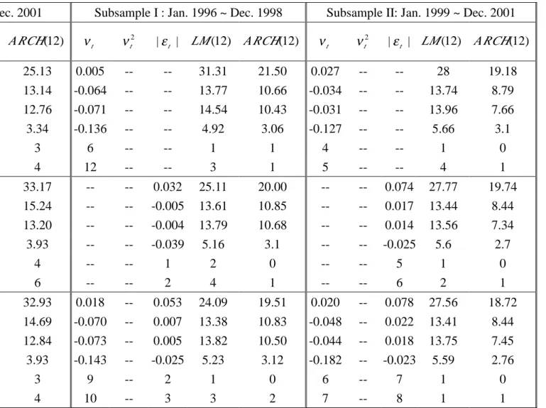
Table 3. Summary Statistics of Estimated Parameters

All Sample: Jan. 1996 ~ Dec. 2001 Subsample I : Jan. 1996 ~ Dec. 1998 Subsample II: Jan. 1999 ~ Dec. 2001 ) 12 ( LM ARCH(12) ν_t 2 t ν |ε_t | LM(12) ARCH(12) ν_t 2 t ν |ε_t | LM(12) ARCH(12) 19.9 25.13 0.005 -- -- 31.31 21.50 0.027 -- -- 28 19.18 12.53 13.14 -0.064 -- -- 13.77 10.66 -0.034 -- -- 13.74 8.79 13.01 12.76 -0.071 -- -- 14.54 10.43 -0.031 -- -- 13.96 7.66 6.14 3.34 -0.136 -- -- 4.92 3.06 -0.127 -- -- 5.66 3.1 0 3 6 -- -- 1 1 4 -- -- 1 0 1 4 12 -- -- 3 1 5 -- -- 4 1 18.33 33.17 -- -- 0.032 25.11 20.00 -- -- 0.074 27.77 19.74 12.32 15.24 -- -- -0.005 13.61 10.85 -- -- 0.017 13.44 8.44 12.85 13.20 -- -- -0.004 13.79 10.68 -- -- 0.014 13.56 7.34 6.13 3.93 -- -- -0.039 5.16 3.1 -- -- -0.025 5.6 2.7 0 4 -- -- 1 2 0 -- -- 5 1 0 0 6 -- -- 2 4 1 -- -- 6 2 1 17.88 32.93 0.018 -- 0.053 24.09 19.51 0.020 -- 0.078 27.56 18.72 12.07 14.69 -0.070 -- 0.007 13.38 10.83 -0.048 -- 0.022 13.41 8.44 12.29 12.84 -0.073 -- 0.005 13.82 10.50 -0.044 -- 0.018 13.75 7.45 5.87 3.93 -0.143 -- -0.025 5.23 3.12 -0.182 -- -0.023 5.59 2.76 0 3 9 -- 2 1 0 6 -- 7 1 0 1 4 10 -- 3 3 2 7 -- 8 1 1

20.41 33.11 0.143 0.094 0.051 24.78 20.86 0.137 0.066 0.078 27.49 18.51 12.04 14.65 -0.075 0.018 0.006 13.30 11.17 -0.036 0.012 0.023 13.34 8.48 12.07 13.04 -0.065 0.020 0.005 13.68 10.44 -0.038 0.005 0.019 13.51 7.78 5.89 3.88 -0.329 -0.084 -0.025 5.28 3.24 -0.188 -0.028 -0.022 4.82 2.76 0 3 7 3 3 1 0 4 1 8 1 0 1 3 9 6 3 3 2 4 1 8 1 0