以靜態機率模型分析為基礎之應用於快速傅利葉轉換處理器設計的精度最佳化技術

國立交通大學

電子工程學系 電子研究所碩士班

碩 士 論 文

以靜態機率模型分析為基礎之應用於快速傅利葉轉

換處理器設計的精度最佳化技術

Precision Optimization for FFT Processor Design using Static

Probability-Based Analysis

研 究 生：石銘恩

指導教授：周景揚 博士

以靜態機率模型分析為基礎之應用於快速傅利葉轉

換處理器設計的精度最佳化技術

Precision Optimization for FFT Processor Design using

Static Probability-Based Analysis

研究生：石銘恩 Student: Ming-En Shih

指導教授：周景揚 教授 Advisor: Jing-Yang Jou

國立交通大學

電子工程學系 電子研究所

碩士論文

A Thesis

Submitted to Department of Electronics Engineering & Institute of Electronics College of Electrical & Computer Engineering

National Chiao Tung University in Partial Fulfillment of the Requirements

for the Degree of Master

in

Electronics Engineering & Institute of Electronics

June 2011

Hsinchu, Taiwan, Republic of China

以靜態機率模型分析為基礎之應用於快速傅利葉轉換處理

器設計的精度最佳化技術

研究生：石銘恩 指導教授：周景揚 博士

國立交通大學

電子工程學系 電子研究所碩士班

摘 要

正交頻分多工系統被廣泛的使用於現今的設計，過去幾十年間可以找到許多關於正 交頻分多工計算核心的快速傅利葉轉換處理器的研究資料。這篇論文描述一個應用於正 交頻分多工系統的計算核心的快速傅利葉轉換處理器設計的精度最佳化流程，藉由決定 每一級的尺規行為來得到最佳化的訊號對量化雜訊比。此方法利用機率分佈來建立每一 級輸出信號的靜態行為模型。由無條件捨去法以及飽和算法的雜訊可以因此被分析，而 做出小數點位置的決定。我們提出的這種方法不但不用很花費時間的模擬分析，而可以 在很短的時間內，固定每一級的數字格式並得到最佳化的訊號對量化雜訊比。這種最佳 化流程可以處理不同的快速傅利葉轉換點數、快速傅利葉轉換演算法、字元長度以及輸 入的機率分佈。實驗結果顯示我們的方法可以在 8192 點、以 2 為基數的快速傅利葉轉 換處理器中，跟傳統的靜態尺規化分析方法比較，節省 3 位元的字元長度，而不增加任 何硬體複雜度。精度更是非常接近動態尺規化方法。

Precision Optimization for FFT Processor Design using

Static Probability-Based Analysis

Student：Ming-En Shih Advisor：Dr. Jing-Yang Jou

Department of Electronics Engineering

Institute of Electronics

National Chiao Tung University

ABSTRACT

As OFDM-based systems are widely adopted in today’s designs, many literatures of FFT processors, the arithmetic kernel of OFDM-based systems, can be found in the past decades. For a high performance FFT processor, many parameters should be decided carefully. In this thesis, we proposed a precision optimization flow to decide the scaling behavior at each stage with optimized output SQNR for FFT processor. The methodology utilizes the probability distribution to model the statistical behavior of the output at each stage. The noise from truncation and saturation arithmetic can be further analyzed to make the scaling decision. Without time-consuming and pattern-dependent simulations, the proposed method fixes the number format at each stage in a short time that gives optimized SQNR. The optimization flow has ability to handle different FFT sizes, FFT algorithms, wordlengths, and distributions of input signals. Experimental results designate that about 3 bits wordlength can be saved in 8K-point, radix-2 FFT processor, with no increasing in hardware complexity compared to traditional static scaling method. Furthermore, the precision is very close to the dynamic scaling method.

Acknowledgements

I deeply appreciate my advisors, Dr. Jing-Yang Jou and Dr. Juinn-Dar Huang, for their patient guidance, valuable suggestion, and encouragement during these years. I am also grateful to Bu-Ching Lin for the discussion and help on my research. Specially thank to all member of EDA Lab and Adar Lab for the great time during path two years. Finally, I would like to express my sincerely acknowledgements to my family and my friends for their patient and support.

Contents

摘 要 ... i ABSTRACT ... ii Acknowledgements ... iii Contents ... iv List of Figures ... vi

List of Tables ... viii

Chapter 1 Introduction ... 1

2.2.1 Memory-based Architectures ... 9

2.2.2 Pipeline-based Architectures ... 10

2.3 Scaling Method ... 11

Chapter 3 The Proposed Approach ... 15

3.1 Motivation ... 15

3.2 Problem Formulation ... 17

3.3 Probability Model ... 18

3.3.1 Probability Mass Function ... 18

3.3.2 Derived Distribution for the FFT Computation ... 20

3.3.3 Saturation Analysis ... 22 3.3.4 SQNR Calculation ... 23 3.4 Scaling Optimization ... 25 3.4.1 Truncation Operation ... 25 3.4.2 Saturation Operation ... 26 3.4.3 Scaling Decision ... 27

3.4.4 The Scaling Optimization Flow ... 29

4.1 SQNR with Different Scaling Behaviors ... 30

4.2 Optimized Scaling Behavior for 8192-point FFT ... 34

Chapter 5 Conclusion and Future Work ... 30

References ... 40

Vita... 42

List of Figures

Fig. 1 Simplified block diagram of OFDM transmitter/receiver ... 1

Fig. 2 First stage of the decimation-in-time FFT algorithm for 8-point DFT ... 6

Fig. 3 The butterfly of a radix-2 DIT FFT algorithm ... 6

Fig. 4 The signal flow graph of the 8-point DIT FFT algorithm ... 6

Fig. 5 The butterfly of a radix-4 DIT FFT algorithm ... 7

Fig. 6 An example of the memory-based architecture ... 10

Fig. 7 The R2SDF architecture for 16-point FFT ... 10

Fig. 8 Butterfly showing scaling by 1/2 at the input ... 11

Fig. 9 Butterfly showing scaling by 1/2 at the output ... 12

Fig. 10 Comparison of different scaling positions, wordlength = 12 bits ... 12

Fig. 11 The SQNR for different σ with 12-bits, 8192-point FFT ... 13

Fig. 12 The scaling behavior for each stage with the approach of [12] ... 15

Fig. 13 The scaling behavior for 256-point FFT with the approach of [12] ... 16

Fig. 14 The PMF of an input random variable with wordlength = 6 bits ... 20

Fig. 15 The butterfly computation ... 21

Fig. 16 The calculation of the addition of two independent uniform random variables ... 21

Fig. 17 The derived distribution in the signal flow of the FFT computation ... 22

Fig. 18 (a) The PMF before saturation with 5-bit integer part (b) The PMF after saturation to 4-bit integer part ... 22

Fig. 19 The PMF behavior of butterfly computation, and the input and output format are <1, 1> and <2, 1>, respectively. ... 26

Fig. 20 The PMF after truncation operation ... 26

Fig. 21 The PMFs of different scaling decisions ... 27

Fig. 23 The proposed optimization flow ... 29 Fig. 24 The SQNR of all possible scaling behaviors for 256-point, radix-2 FFT with 12-bit wordlength ... 31 Fig. 25 SQNR vs. FFT sizes with different scaling approaches for radix-2 FFT algorithm .... 33 Fig. 26 SQNR vs. FFT sizes with different scaling approaches for radix-4 FFT algorithm .... 33 Fig. 27 SQNR vs. FFT sizes with different scaling approaches for radix-8 FFT algorithm .... 33 Fig. 28 SQNR vs. wordlength for 8192-point, radix-2 FFT ... 35 Fig. 29 SQNR vs. wordlength for 8192-point, radix-4 FFT ... 36 Fig. 30 SQNR vs. wordlength for 8192-point, radix-8 FFT ... 37 Fig. 31 SQNR vs. wordlength for 8192-point, radix-4 FFT with normally distributed inputs (σ= 0.2) ... 37 Fig. 32 SQNR vs. wordlength for 8192-point, radix-4 FFT with normally distributed inputs (σ= 0.4) ... 38 Fig. 33 SQNR with different deviations for 8192-point, radix-4 FFT with normally distributed inputs (WL = 12) ... 38

List of Tables

Table I Nontrivial complex multiplications required for radix-2, radix-4, and radix-8 FFT algorithm ... 9 Table II 64-Point FFT Output Format Analysis ... 24 Table III The comparison between analysis method and simulation method ... 24 Table IV Precision rank of all possible scaling behaviors for 256-point, radix-2 FFT with 12-bit wordlength ... 32 Table V Scaling behavior for 8192-point, radix-2 FFT ... 34 Table VI Hardware Comparison of 11-bit and 14-bit wordlength for 8192-point, radix-2 FFT ... 36

Chapter 1

Introduction

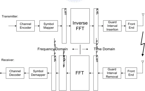
Recently, high-data-rate wireless communication systems are the focus of research and development. Orthogonal Frequency Division Multiplexing (OFDM) technology is one of the favorable choice for future broadband system and very suitable for video transmission and mobile Internet applications such as digital video/audio broadcasting (DVB/DAB) [1], local area network (IEEE 802.11a/g/n) [2], and network for multiple users (IEEE 802.16, WiMAX, LTE) [3-5]. As is well known, the Fast Fourier Transform (FFT) processors are one of the key components in OFDM-based wireless system [4, 6, 7]. The simplified block diagram of OFDM is shown in Fig. 1. In [8], the authors showed through extensive simulation that the most computationally intensive parts of such a high-data-rate system are the FFT core. Therefore, many literatures have been reported on FFT processor design nowadays.

Channel

Encoder Symbol Mapper

Se ria l t o Pa ra Inverse FFT Pa ra lle l t o Se r Guard Interval Insertion Front End Channel

Decoder DemapperSymbol

Pa ra lle l t o Se tia l FFT Se ria l t o Pa ra lle l Guard Interval Removal Front End O ne -tap E qu al lz er Transmitter: Receiver: Time Domain Frequency Domain

The architectures of FFT processors can be divided into two main categories: 1) memory-based architectures and 2) pipeline-based architectures. Memory-based architectures usually consist of a butterfly unit and certain number of memory blocks for providing an area-efficient design. Alternatively, a pipelined architecture consists of multiple stages to provide higher throughput at the cost of more hardware. In general, memory-based architectures are suitable for low hardware cost and long-size FFT processors whose size is not smaller than 512 [3]. And the pipeline-based architectures are feasible for short-size and high throughput applications. In this work, we focus on the FFT design with fixed wordlength at each stage, that is, the output wordlengths of every stages are the same as input signals. The memory-based architectures are under this constrain for sure. However, it is not limited for memory-based FFT. For many pipeline-based architectures, the fixed wordlength is also preferred due to the considerations of the hardware cost and the critical-path delay [9].

Taking the actual hardware design into consideration, the precision in terms of Signal to Quantization Noise Ratio (SQNR) is a significant design factor of system performance [10]. Conducting the addition and subtraction operations may cause overflows during FFT computations. In practice, the FFT algorithms are implemented by fixed-point arithmetic since the resolution of coefficients and operations cannot be infinite. Finite number of bits in binary format is used to represent all signals and coefficients. As a result, rounding or truncation operations introduce noise which is referred as quantization noise. Besides, conducting the addition and subtraction operations may cause overflows during FFT computations. Although increasing wordlength can be used to avoid accuracy loss [11], the hardware cost and the critical-path delay are increased accordingly.

Therefore, many scaling methods have been proposed for an efficient FFT processor which meets SQNR requirement with the fixed-wordlength constrain [1, 7, 9, 12-14]. Oppenheim et al. [12] proposed a basic scaling method which is scaling by 1/2 for each radix-2 stage. Since the scaling factor is trivial to implement, the approach is the simplest scaling method. We define a

scaling method with a constant scaling factor as a static scaling method. Besides, the Block Floating Point (BFP) [14] and its variants [1, 7, 9, 14, 15] employ intermediate buffers to store the output data, and decides the output format appropriately to maximally utilize the dynamic range which gets good SQNR. However, these methods have a penalty in terms of area, power, latency, and complex control unit. This kind of methods is called the dynamic scaling method. Due to the increased complexity of BFP, traditional scaling optimization methods rely on time-consuming simulations to fix a static scaling behavior at each stage [13].

In this thesis, we propose a static scaling optimization flow to quickly decide the number format at each stage to optimize the SQNR with given probability distribution of input signals, FFT algorithm, and wordlength. For the same SQNR requirement, smaller wordlength is needed in an FFT processor with no increase in complexity compared to existing static designs [12, 13].

The remainder of this thesis is organized as follows. In Chapter 2, we briefly review the fundamentals of FFT algorithm and architecture. The proposed static scaling optimization flow is demonstrated in Chapter 3. Chapter 4 shows our experimental setup and presents the experimental results. Finally, Chapter 5 gives the concluding remarks of this thesis.

Chapter 2

Preliminaries

In this chapter, we will review FFT algorithms, FFT architectures, and the scaling consideration in FFT hardware design.

2.1 The FFT Algorithm

Since the FFT algorithm was proposed by Cooley and Turkey in 1965 [16], many similar algorithms have been developed to reduce the computational complexity of FFT [17-19]. To structure the DFT computation by forming increasingly smaller subsequences of the input sequence x(n) is called a decimation-in-time (DIT) FFT algorithm. Alternatively, using a first-half and second-half approach which divides the output sequence X(k) into increasingly smaller subsequences to decompose the DFT computation is called a decimation-in-frequency (DIF) FFT algorithm [20]. Because both of these algorithms are similar in nature, the DIT algorithm is used to illustrate the FFT algorithm in our thesis.

We will introduce the radix-2/4/8 DIT FFT algorithm, and the general form, that is, radix-r DIT FFT algorithm, where r is 2s for s is any positive integer. Furthermore, the computational complexity of the radix-r FFT algorithms will be compared.

2.1.1 Radix-2 DIT FFT Algorithm

An FFT is an efficient algorithm to compute the Discrete Fourier Transform (DFT). The formulation of N-point DFT is define as

X(k) = ∑N−1n=0x(n)WNnk, k = 0,1, … , N − 1 (2.1)

where x(n) and X(k) are complex numbers, and the coefficient W_Nnk= e−j2πnkN = cos �2πnk

N � − j sin � 2πnk

Radix-2 Decimation-In-Time (DIT) FFT Algorithm divided x(n) into its even- and odd- numbered points and substitute n=2r for n is even, n=2r+1 for n is odd.

X(k) = � x(2r)W_N(2r)k N 2−1 r=0 + � x(2r + 1)WN (2r+1)k N 2−1 r=0 = ∑ x(2r)WN2rk N 2−1 r=0 + WNk∑ x(2r + 1)WN2rk N 2−1 r=0 (2.2)

Since W_N2 =W_N/2, (2.2) can be rewritten as

X(k) = ∑ x(2r)WN/2rk N 2−1 r=0 + WNk∑ x(2r + 1)WN/2rk N 2−1 r=0 (2.3)

Each of the sums in (2.3) can be recognized as an N/2-point DFT. The first term is the N/2-point DFT of the even-numbered points of the original sequence and the second term is the odd-numbered points shown in Fig. 2. Then we divide k into k and k+N/2, for k = 0, 1, …, N/2-1. Because W_NN/2 = e−j�2πN�N2 = e−jπ = −1 and W_Nr+N/2 = W_NN/2W_Nr = −W_Nr. Equation (2.3) can be rewritten to X(k) = ��x(2r) + WNkx(2r + 1)� N 2−1 r=0 WN/2rk X �k +N₂� = ∑ �x(2r) − WNkx(2r + 1)� N 2−1 r=0 WN/2rk (2.4)

Through log2N-time recursive decompositions, we can complete an N-point FFT. As a

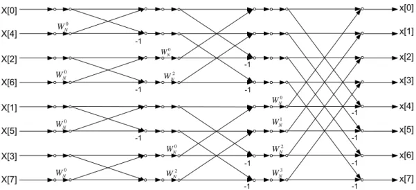
result, the FFT computation can be computed by a butterfly shown in Fig. 3. The whole signal flow for the 8-point DIT FFT computation is shown in Fig. 4. From (2.1), we can find that the complexity of multiplications in DFT is N2. After the decompositions of FFT, the complexity of multiplications becomes N/2*(log2N-1) and the complexity of additions and subtractions is

N/2-Point

DFT

X[0] X[4] X[2] X[6] X[1] X[5] X[3] X[7] x[0] x[1] x[2] x[3] x[4] x[5] x[6] x[7] -1 -1 -1 -1 4 N W 6 N W 5 N W 7 N W

N/2-Point

DFT

0 N W 2 N W 1 N W 3 N W

Fig. 2 First stage of the decimation-in-time FFT algorithm for 8-point DFT

+

-Xm-1[p] r N W

*

Xm-1[q] Xm[p] Xm[q] Fig. 3 The butterfly of a radix-2 DIT FFT algorithm

x[0] x[1] x[2] x[3] x[4] x[5] x[6] x[7] X[0] X[4] X[2] X[6] X[1] X[5] X[3] X[7] -1 -1 -1 -1 -1 -1 -1 -1 -1 -1 -1 0 N W 0 N W 0 N W 0 N W 0 N W 0 N W 0 N W 2 N W 2 N W 2 N W 1 N W 3 N W

2.1.2 Radix-4 DIT FFT Algorithm

Similar to radix-2 FFT algorithm, we can also use 4-point DFT to decompose N-point FFT, which is called the radix-4 FFT algorithm. We split the N-point input signals into four subsequences, x(4n), x(4n+1), x(4n+2), x(4n+3), r = 0, 1, …, N/4-1, and the N-point DFT, with dividing k into k, k+N/4, k+2N/4, k+3N/4, for k=0, 1, …, N/4-1, can be rewritten as

X(k) = � �x(4n) + WNkx(4n + 1) + WN2kx(4n + 2) + WN3kx(4n + 3)� N 4−1 n=0 WN/4 nk X(k + N/4) = � �x(4n) − jWNkx(4n + 1) − WN2kx(4n + 2) + jWN3kx(4n + 3)� N 4−1 n=0 WN/4 nk X(k + 2N/4) = � �x(4n) − WNkx(4n + 1) + WN2kx(4n + 2) − WN3kx(4n + 3)� N 4−1 n=0 WN/4 nk X(k + 3N/4) = ∑ �x(4n) + jWNkx(4n + 1) − WN2kx(4n + 2) − jWN3kx(4n + 3)� N 4−1 n=0 WN/4nk (2.5) Equation (2.5) illustrates the radix-4 butterfly computation as shown in Fig. 5. The complexity of multiplications in the radix-4 FFT algorithm is 3/4N*(log4N-1), which is lower

than radix-2, as the complexity of additions and subtractions is Nlog2N, which is the same as

that of radix-2. 0 N

W

1 N

W

2 N

W

3 N

W

2.1.3 Radix-8 DIT FFT Algorithm

Compared to the radix-2 and radix-4 FFT algorithms, the radix-8 FFT algorithm can further reduce the complexity of multiplications. The general from is

X �k +qN₈ � = ∑ W₈pqW_Npk∑ X(8n + p)WN/8nk N 8−1 n=0 7 p=0 (2.6)

where q=0, 1, …, 7. The complexity of multiplications is 7N

8 ∗ (log8N − 1).

2.1.4 Radix-r DIT FFT Algorithm

For general cases, we derive the radix-r DIT FFT algorithm, where r is 2s, and s is any positive integer. For N-point DFT, the general form is

X �k +qN_r � = ∑ WrpqWNpk∑ X(rn + p)WN/rnk N r−1 n=0 r−1 p=0 (2.7)

where q=0, 1, …, r − 1. The complexity of multiplications is (s−1)N

s ∗ (logsN − 1).

2.1.5 Comparison of Radix-r DIT FFT Algorithms

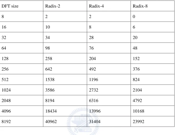
Table I shows the nontrivial complex multiplication required for radix-2, radix-4, and radix-8 algorithm [17]. Since the number of stages is logr N, where r is the radix number, the

higher-radix FFT algorithm has lower complexity of multiplications obviously. The radix-8 FFT algorithm has only about half of complex nontrivial complex multiplications compared to the radix-2 FFT algorithm, as listed in Table I. Nevertheless, higher hardware cost is required for the implementation of higher-radix butterfly unit. For example, the butterfly unit of the radix-8 FFT algorithm needs 7 nontrivial complex multipliers, while the butterfly unit of radix-2 FFT algorithm needs only 1 complex multiplier. Designers have to choose the feasible algorithm to optimize area, power consumption, and throughput.

Table I Nontrivial complex multiplications required for radix-2, radix-4, and radix-8 FFT algorithm

DFT size Radix-2 Radix-4 Radix-8

8 2 2 0 16 10 8 6 32 34 28 20 64 98 76 48 128 258 204 152 256 642 492 376 512 1538 1196 824 1024 3586 2732 2104 2048 8194 6316 4792 4096 18434 13996 10168 8192 40962 31404 23992

2.2 The FFT Architecture

The architectures of FFT processors can be divided into two main categories: 1) memory-based architectures and 2) pipeline-based architectures. In general, memory-based architectures are suitable for low hardware cost and long-size FFT processors whose size is not smaller than 512 [3]. And the pipeline-based architectures are feasible for short-size and high throughput designs. More details are introduced in the following subsections.

2.2.1 Memory-based Architectures

Memory-based architectures are the simplest FFT architecture, as shown in Fig. 6. General speaking, it consists of a storage and a processing element (PE) which contains one or few butterflies (BF). Data are read from the storage and computed in the PE. After the

number of stages for the N-point FFT computation is logr N. The number of butterflies and the

algorithm in the processing element can be chosen freely to meet the throughput rate requirement. To solve the problem of the memory bandwidth, the generalized conflict-free addressing schemes for memory-based FFT architectures are presented in [21, 22].

Control Unit

Memory

Mux Radix-r PE Mux

Fig. 6 An example of the memory-based architecture

2.2.2 Pipeline-based Architectures

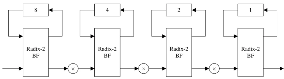
Pipeline-based architectures are usually regular, modular, local connection, and high throughput rate with higher hardware complexity [23]. In general, pipeline-based architectures can be divided into two types of architectures, which are the Single-path Delay Feedback (SDF) FFT architecture [24, 25] and the Multi-path Delay Commutator (MDC) [26] architecture. Take the SDF architecture as an example, the radix-2 SDF (R2SDF) architecture is shown in Fig. 7. The R2SDF can use the registers very efficiently by storing half of the butterfly output into the shift register while the other half of output is passing to the next stage. That is, only one output passes to the next stage in each cycle.

Radix-2 BF × Radix-2 BF Radix-2 BF Radix-2 BF 8 4 2 1 × ×

2.3 Scaling Method

Because of the addition and subtraction operations in FFT computations, the value range is increased from stage to stage. One solution to avoid possible overflows in a fixed-point FFT design is to increase the wordlength [11]. However, the increased wordlength has many drawbacks in FFT implementations. First, a larger storage is required to store the data which increases both chip area and power consumption. Second, a longer wordlength results in worse critical-path timing for the arithmetic units, which is not preferred in the high-throughput FFT designs. The most of all, the wordlength is fixed in the memory-based FFT architecture which cannot allow different wordlengths from stage to stage. Consequently, many scaling methods have been proposed for FFT processors to scale the data for wordlength reduction. The scaling scheme for fixed-point FFT processors can be roughly divided into two categories: 1) Static Scaling Method and 2) Dynamic Scaling Method.

Oppenheim et al. [12, 20] suggest a static scaling procedure which is easy to understand, simple to implement, and most often used. Since the maximum magnitude increases by no more than a factor of 2 from stage to stage, we can prevent overflow by incorporating an attenuation of 1/2, that is, increase 1 bit for integer-part and decrease 1 bit for fraction-part, at the input to each butterfly, as shown in Fig. 8. In this case, the SQNR may not as good as the dynamic scaling method, but the hardware is very simple to implement.

+

-Xm-1[p] r N W 2 1

*

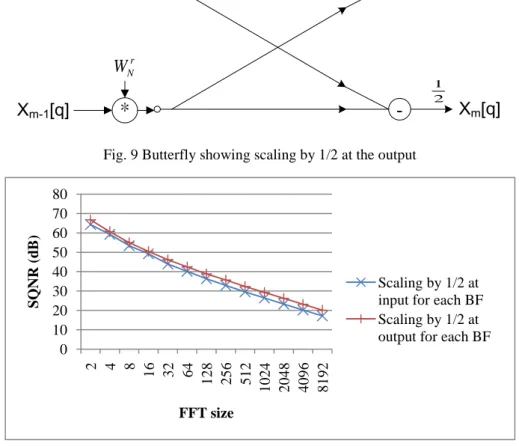
2 1 Xm-1[q] Xm[p] Xm[q] Fig. 8 Butterfly showing scaling by 1/2 at the input

SQNR. Since the original method induces the noise at the input of each butterfly, the accuracy will be lost from the beginning. We modify the butterfly of Fig. 8 to that of Fig. 9, where the output is noiseless before scaling. Fig. 10 shows the simulation result of two methods. We can see that scaling at the output is always a better choice.

+

-Xm-1[p] r N W 2 1

*

2 1 Xm-1[q] Xm[p] Xm[q] Fig. 9 Butterfly showing scaling by 1/2 at the output

Fig. 10 Comparison of different scaling positions, wordlength = 12 bits

In [13], Ramakrishnan et al. consider a special case of FFT design for OFDM receivers. The authors exploit the Gaussian nature of OFDM signals to predict the growth of the value range of signals at each stage and decide the scaling behavior appropriately. They suggest increasing 1 bit of integer parts for every two stages instead of every stage. However, the model of Gaussian distributed inputs is not suitable for general case, like uniformly distributed input which is most assumed in FFT analysis [11, 12]. Furthermore, the method has good results only in a small range of σ of Gaussian distribution. Fig. 11 shows the SQNR for different σ with the two methods.

0 10 20 30 40 50 60 70 80 2 4 8 _{16 32 64} 128 256 512 1024 2048 4096 8192 SQ N R ( dB ) FFT size Scaling by 1/2 at input for each BF Scaling by 1/2 at output for each BF

Fig. 11 The SQNR for different σ with 12-bits, 8192-point FFT

The other way to do the static scaling optimization is through time-consuming and pattern-dependent simulations to find feasible number formats for each stage. Since the exhaustive simulation is impractical in many cases, designers usually intuitively pick some configurations to evaluate, and choose the best one among them.

The dynamic scaling method uses a shard-exponent concept which not only reduces the wordlength in FFT processors but also acquires good SQNR. The block floating point (BFP) algorithm [1, 14, 20], which is one of the dynamic scaling approaches, employs intermediate buffers to store the output data, and detects the maximum value to decide the exponent for each buffer. Unfortunately, the intermediate buffers and exponent storage causes a large amount of area overhead. Also, the additional processing latency and power consumption are introduced by the intermediate buffer accesses and data detections. Due to the increased complexity of the dynamic scaling method, the static scaling approach is preferred for many FFT designs in reality.

We propose a static scaling optimization method to maximize the precision in terms of SQNR. Not only the hardware complexity is the same as that of the traditional static scaling method, but also the precision comes close to the dynamic scaling method. Our method

0.00 5.00 10.00 15.00 20.00 25.00 30.00 35.00 40.00 45.00 50.00 SQ N R ( dB ) deviation σ Ramakrishnan [13] Oppenheim [12]

truncation and saturation operations. It can suggest the number format for each stage in a short time, and also can handle different FFT sizes, FFT algorithms, wordlengths, and distributions of input signals.

Chapter 3

The Proposed Approach

This chapter has four sections. The first one describes the motivation of static scaling optimization. And the second one defines the problem formulation. In the third section, we illustrate the probability model and the derived distribution with the computation in FFT. Last, we present the proposed static scaling optimization method. The purpose of this thesis is to fix the scaling behavior at each stage with optimized SQNR in short time.

3.1 Motivation

With the approach of [12], the integer-part bit would be increased by 1 for each butterfly. Fig. 12 shows the general form of the scaling behavior for each stage with the radix-2 FFT algorithm. Note that a stage is a radix-2 butterfly computation and the format <m, n> means a 2’s complement binary number with m bits for integer-part and n bits for fraction-part, where m + n = WL (total wordlength). The number of representable values is 2WL. When m is increased by 1, the scale of representable values is double. The n is then decreased by 1, so the precision is decreased. Take the radix-2 64-point FFT with <1, 11> input format as an example, it has log2 64 = 6 stages, therefore the output format would be <7, 5>.

Stage s

<s, WL-s> <s+1, WL-s-1>

Fig. 12 The scaling behavior for each stage with the approach of [12]

However, through 21.6M sets of 64-pt FFT simulation which takes 12 hours to run, the probability that need 7 bits for integer-part is about 0%. That is, we may use fewer bits for

integer-part to acquire better SQNR since more bits for fraction-part are reserved. To handle the possible overflow problems, we apply saturation arithmetic which is a common technique in DSP computation to reduce the noise.

Saturation arithmetic is an arithmetic to limit a number to a fixed range between a minimum and maximum value. For example, if the valid range is from -8 to 7 (4 bits for integer-part), the overflow occurs when we compute 2’b0100 (4) + 2’b0101 (5) = 2’b1001 (-7). The noise would be 9 – (-7) = 16 since the correct answer is 9. If we apply saturation arithmetic, the result would be saturated to 7 when the correct answers larger than 7. So the error is 9–7 = 2 which is much smaller than 16.

We illustrate an example of static scaling optimization. Fig. 13 shows a configuration which is the traditional scaling behavior of 256-point FFT and the SQNR is 35.39 dB. If we modify the output format at Stage 8 from <9, 3> to <8, 4>, the SQNR would be increased to 37.03 dB. And we further modify the output format at stage 7 from <8, 4> to <7, 5>, the SQNR would be increased to 38.47 dB. However, if we further modify the output format at stage 2 from <3, 9> to <2, 10>, the SQNR would be decreased to 17.82 dB. The example tells that the format of each stage has to be chosen appropriately to get the best SQNR.

Stage 1 Stage 2 Stage 3 Stage 4

Stage 5 Stage 6 Stage 7 Stage 8 Input <1, 11> <2, 10> <3, 9> <4, 8> <5, 7> <6, 6> <7, 5> <8, 4> Output <9, 3>

Fig. 13 The scaling behavior for 256-point FFT with the approach of [12]

Traditional static scaling optimization method has relied on time consuming simulations to fix the scaling behavior at each stage [13]. Nevertheless, it costs about 80 hours to simulate only 10k sets of 8192-point FFT for one configuration. And for the radix-2 FFT algorithm, since each stage has to be decided increasing 1 bit of integer-part or not, 8192 possible

configurations exist. It needs about 75 years to do the simulation which is very impractical. As a result, we propose a static scaling optimization approach which can fix the scaling behavior in less than 2 minutes in this thesis.

3.2 Problem Formulation

To define the precision optimization problem, we illustrate the problem as follow: Given FFT size, radix-r FFT algorithm where r is the power of 2, wordlength for both I/O and storage, and the input probability distribution, the static scaling optimization problem is to fix the number format at each stage to give the maximum SQNR for the whole fixed-point FFT computation.

3.3 Probability Model

3.3.1 Probability Mass Function

In order to do the analysis, we model the input as a discrete random variable (RV) which is real and its number of values is finite. For a discrete random variable X, it has an associated

probability mass function (PMF) [27], which gives the probability of each numerical value

that the random variable can take, denoted pX. In particular, if x is any possible value of X, the

probability mass of x, denoted pX(x), is the probability of the event {X = x} (P({X = x}) for

short) consisting of all outcomes that give rise to a value equal to x:

pX(x) = P({X = x}) (3.1)

Note that

∑ 𝑝_{x X}(𝑥)= 1 (3.2) where in the summation above, x ranges over all the possible numerical values of X.

Since the input of an FFT processor is a fixed-point complex number, the wordlength (WL) for both real and imaginary parts of the signals are fixed. That is, the number of the representable value is numerical which is restricted to 2WL for 2’s complement binary number. For example, 2 bits number with <1, 1> format has 22=4 representable values which are {-1, -0.5, 0, 0.5}. As a result, the PMF can perfectly describe the behavior of signals in terms of the probability of each representable value in fixed-point design.

Besides, computing either real part or imaginary part of input signals can represent the total result in terms of SQNR, which is proved below.

Theorem 1

In FFT computation, computing either real part or imaginary part of input signals can represent the total result in terms of SQNR if the real part and imaginary part of the input signals have the same probability distribution.

For N-point FFT, x[n] is the input sequence which has N element and y[k] is the FFT of x[n] where

y[k] = ∑N−1n=0x[n]WNnk (3.3)

We first prove that

Powersignal= 2 ∗ Powersignal_real (3.4)

For each element in y, denoted y[k], we have

Powery = |y[k]|2 = ��∑N−1n=0𝑥[n]WNnk��2= �∑N−1n=0|𝑥[n]|�WNnk��2 (3.5)

Since W_Nnk is on the unit circle and its magnitude is unary, that is

�WNnk� = 1 (3.6)

Equation (3.5) can be rewritten to

|y[k]|2 _{= �∑}N−1_|𝑥[n]|

n=0 �2 = �∑N−1n=0�𝑥𝐼[n] + 𝑗 ∗ 𝑥𝑄[n]��2 (3.7)

where 𝑥_𝐼[n] is the real part and 𝑥_𝑄[n] is the imaginary part.

Since 𝑥_𝐼[n] and 𝑥_𝑄[n] have the same distribution, in average, Eq. (3.7) becomes |y[k]|2 _{= �∑ �2𝑥} 𝐼[n]2 N−1 n=0 � 2 = 2 ∗ �∑N−1n=0𝑥𝐼[n]�2 (3.8)

And from the computation with real part of the input sequence y_real, we have

|yreal[k]|2 = �∑N−1n=0𝑥𝐼[n]�2 (3.9)

Combing Eq. (3.8) and Eq. (3.9), we obtain |y[k]|2 = 2|y_real[k]|2, which guarantees Eq. (3.4).

The power of noise can also be proved that

Powernoise= 2 ∗ Powernoise_real (3.10)

From Eq. (3.4) and (3.10), we can derive that

SQNRtotal = 10 ∗ log10�Power_Powersignal

noise� dB

End of proof

By Theorem 1, we can only analyze the real-part of input signals to represent the complex signals when computing SQNR.

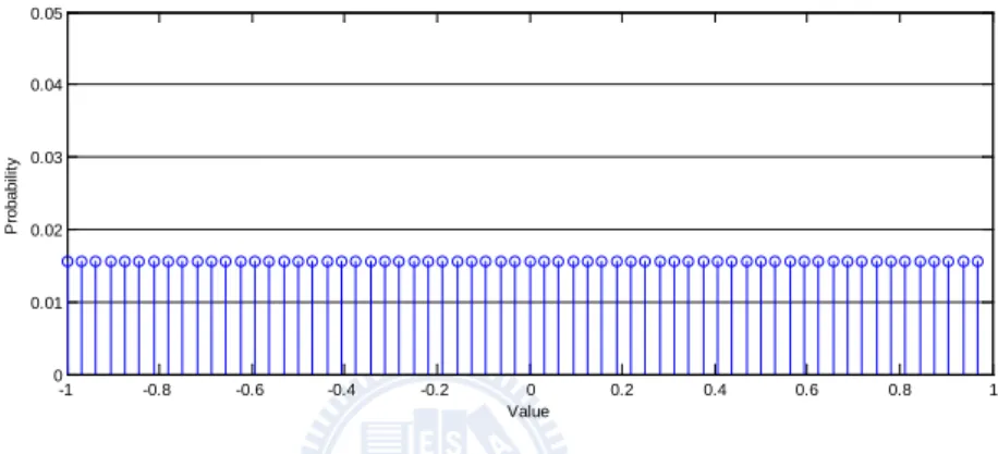
In the following discussion, we assume either real-part or imaginary-part for each input signal of the fixed-point FFT computation is a discrete random variable that is independent with each other and uniformly distributed in [-1, 1). Fig. 14 shows the PMF of an input random variable with the uniform distribution and 6-bit wordlength.

Fig. 14 The PMF of an input random variable with wordlength = 6 bits

3.3.2 Derived Distribution for the FFT Computation

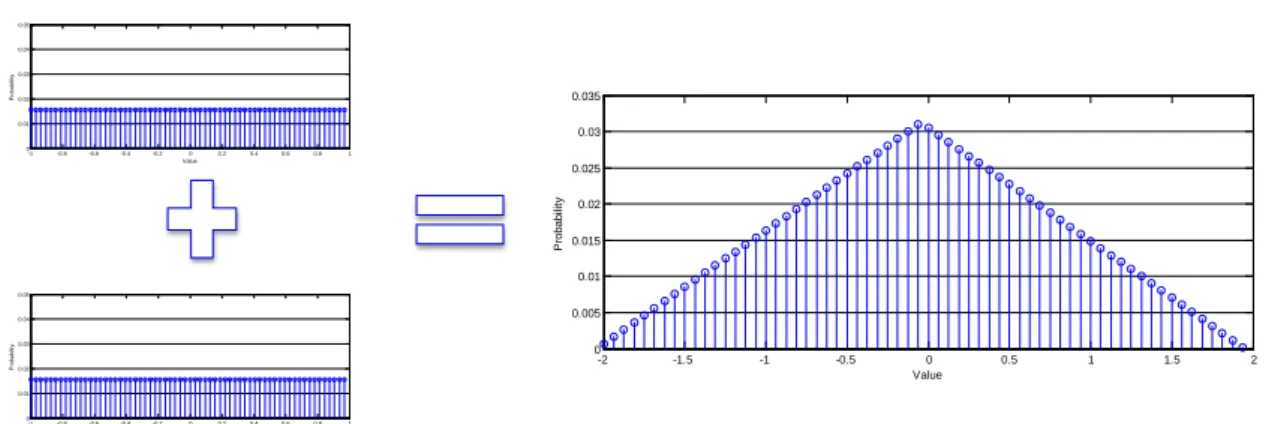
In this section, we consider functions Y = g(X) of a discrete random variable X. Given the PMF of X, we discuss techniques to calculate the PMF of Y (also called a derived distribution) [27]. In order to discuss the derived distribution of the FFT computation, we now focus on the special case where the function g is the FFT computation, denoted fft. A flow graph representing the raidx-2 butterfly computation is shown in Fig. 15, which is the basic computation of FFT. We can observe that the butterfly consists of two operations, which are the addition/subtraction operation and the twiddle factor multiplication operation. If we can handle the two derived distributions of these two operations, we can derive the distribution of the output of the FFT computation at each stage.

-1 -0.8 -0.6 -0.4 -0.2 0 0.2 0.4 0.6 0.8 1 0 0.01 0.02 0.03 0.04 0.05 Value P robabi lit y

+

-Xm-1[p] r N W

*

Xm-1[q] Xm[p] Xm[p] Fig. 15 The butterfly computation

For the addition operation, we now consider an example of a function of two random variables, namely, the case where Z = A + B, for independent A and B with PMFs pA and pB,

respectively. Then for any integer z, we have pZ(z) = P(A + B = z)

= ∑_{{(a,b)|a+b=z}}P(A = a, B = b) = ∑ P(A = a, B = z − b)a

= ∑ px A(a)pB(z − b) (3.12)

The resulting PMF pZ is called the convolution of the PMFs of A and B. See Fig. 16 for

an illustration. And the subtraction operation can be proved that is the same as the addition operation.

Fig. 16 The calculation of the addition of two independent uniform random variables

Since the twiddle factor W is unary, that is, |W| = 1, the scalar has no effect when computing the derived distribution of Y_real[k] = ∑N−1_n=0x_IW_Nnk or Y_imag[k] = ∑N−1_n=0x_QW_Nnk. According to Theorem 1, each of Yreal or Yimag can represent the total FFT computation in

-2 -1.5 -1 -0.5 0 0.5 1 1.5 2 0 0.005 0.01 0.015 0.02 0.025 0.03 0.035 Value P robabi lit y -1 -0.8 -0.6 -0.4 -0.2 0 0.2 0.4 0.6 0.8 1 0 0.01 0.02 0.03 0.04 0.05 Value P robabi lit y -1 -0.8 -0.6 -0.4 -0.2 0 0.2 0.4 0.6 0.8 1 0 0.01 0.02 0.03 0.04 0.05 Value P robabi lit y

propagation of the addition operation. Fig. 17 shows the derived distribution in the 8-point FFT computation. The x-axis is the representable value and the y-axis is the probability of each representable value.

Fig. 17 The derived distribution in the signal flow of the FFT computation

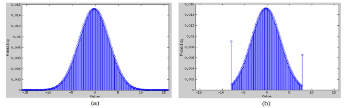
3.3.3 Saturation Analysis

To model the behavior of saturation, we limit the representable value of output between a maximum and a minimum value which are decided by the given output format. For example, if the integer part of the given format is 4 bits, the maximum value is near 8 (smaller than 8 by a fractional unit), and the minimum value is exactly -8. The probability of the overflowed values which are beyond the limited value would be added to the maximum or the minimum value, such that the PMF of output with the behavior of saturation is modeled. The PMF with the behavior of saturation is illustrated in Fig. 18.

Fig. 18 (a) The PMF before saturation with 5-bit integer part (b) The PMF after saturation to 4-bit integer part

x[0] x[1] x[2] x[3] x[4] x[5] x[6] x[7] X[0] -1 -1 -1 -1 -1 -1 -1

3.3.4 SQNR Calculation

In order to calculate the SQNR of the output of FFT, we need to know the power of the fixed-point output and the noise-free output. With the method in 3.3.2, we can get the output derived distribution, denoted p for its PMF, which is assumed that the computation is noise-free. That is, the noise from multiplication and add/subtraction is ignored. However, the output wordlength is fixed to the input wordlength, such that the number of representable value for output is not as much as the representable value in the output derived distribution, denoted x’. Signal x’ would be truncated to x which is representable for output. These point then induce truncation error which is x’-x. Note that the saturation operation also induces error, and the way to calculate its power is as same as truncation error. We can take the overflowed value before saturated as x’, and x would be the value that x’ is saturated to.

For example, if the output derived distribution has the format <2, 1>, the representable value is [-1, -1.5, -1, -0.5, 0, 0.5, 1, 1.5]. But the I/O wordlength is 2 bits, and the output format is <2, 0>, x’: [-1.5, -0.5, 0.5, 1.5] cannot be represented. These values would be truncated to x: [-2, -1, 0, 1], respectively, and induce truncation error by 0.5 for each.

The formula for SQNR calculation is

SQNR = 10 ∗ log10�Power_Powersignal_noise� dB (3.13)

And we can calculate the power of signalby the output derived distribution as

Powersignal = ∑ (𝑥𝑥 2∗ 𝑝(𝑥)) (3.14)

The power of noise can also be calculate by

Powernoise = ∑ ((𝑥𝑥′ ′− 𝑥)2∗ 𝑝(𝑥′)) (3.15)

With Eq. (3.14) and Eq. (3.15), we can evaluate SQNR by Eq. (3.13).

Take a 64-point FFT with 12-bit I/O as an example, we apply four different output formats and calculate their SQNR. The integer part decides the output range, and the fraction part decides the unit. The calculation result is shown in Table II . Note that Unit in the third

column means the smallest number which the format can represent. We can find that <6, 6> has the best SQNR among these output formats, since its overflow probability is near zero and the unit is half compared to <7, 5>.

Table II 64-Point FFT Output Format Analysis

Output Format Output Range Unit SQNR Overflow

Probability

<7, 5> [-64, 63) 0.0313 48.17 dB 0 %

<6, 6> [-32, 31) 0.0156 54.19 dB 5.53*10-11 %

<5, 7> [-16, 16) 0.0078 42.49 dB 0.049 %

<4, 8> [-8, 8) 0.0039 16.14 dB 8.33 %

The proposed SQNR model was verified using the simulation method. The comparison is shown in Table III. In this simulation, the result is from 21.6M randomly sets of 64-point FFT with the uniform distribution. And each of formats cost about 12 hours to simulate by Matlab. As a result, the SQNR difference is smaller than 0.15 dB, and the overflow probabilities evaluated by the two methods are extremely closed.

Table III The comparison between analysis method and simulation method

Output Format Analysis Method Simulation Method Difference

SQNR Overflow Probability SQNR Overflow Probability SQNR Overflow Probability <7, 5> 48.17 dB 0 % 48.17 dB 0 % 0.00 dB 0 % <6, 6> 54.19 dB 5.53*10-11 % 54.20 dB 0 % 0.01 dB ~0 % <5, 7> 42.49 dB 0.049 % 42.34 dB 0.050 % 0.15 dB 0.001 % <4, 8> 16.14 dB 8.33 % 16.13 dB 8.34 % 0.01 dB 0.01 %

3.4 Scaling Optimization

In this section, we further consider the scaling behavior from stage to stage, and illustrate the proposed flow of the scaling optimization. Since the output wordlength is fixed, the representable value of each stage is also the same, and then the scale decision has to be made. Based on the probability model and derived distribution concepts, we propose a greedy algorithm to suggest the scaling behavior at each stage with optimized precision. The modified model is more suitable for fixed-point hardware implementation, and the computation complexity is O(2WL*s), where s is the number of stages and WL is the wordlength.

3.4.1

Truncation Operation

The wordlength is increasing through FFT computation in the butterfly as mentioned. However, the data has to be quantized to write into storage whose wordlength is fixed and as same as the input of butterfly. Truncation operation for quantization is to discard few bits from the least significant bit (LSB) for limiting the number of bits. For example, consider the 5-bit binary number 0.1011 (0.6875) and if we truncate it to 4 bits, the result would be 0.101 (0.625) which is resulting from discarding 1 bit from LSB.

For each radix-2 butterfly, the number of representable values in output is about double compared to the input as shown in Fig. 19. When the truncation operation is applied then, half of values are not representable. To model the probability behavior, the probability of the value which is truncated would be added to the probability of representable value. After the truncation, the PMF in Fig. 19 becomes the PMF shown in Fig. 20. The noise induced by truncation operation can be computed with the method mentioned in Ch. 3.3.4.

Fig. 19 The PMF behavior of butterfly computation, and the input and output format are <1, 1> and <2, 1>,

respectively.

-1.5 -1 -0.5 0 0.5

-2 1 1.5

1/4

Fig. 20 The PMF after truncation operation

3.4.2

Saturation Operation

In addition to the truncation operation, saturation behavior can also be modeled in terms of PMF and noise. With given number range, that is, wordlength of integer part, the maximum and minimum value can be decided. The number beyond the limitation would be saturated to the maximum or minimum value, and its probability is also added to the probability of the maximum or minimum value. The operation is similar to the analysis method mentioned in Ch. 3.3.3. The major difference is that the operation is applied at each stage and evaluated the noise induced for scaling decision.

3.4.3

Scaling Decision

With the two operations and its noise analysis, the noise at each stage can be evaluated with given number format. Take the radix-2 FFT algorithm as an example, there are two scaling choices which are to increase 1 integer bit or to maintain the number format of input from stage to stage. If increasing 1 integer bit is decided, the range of representable value is double, but the fractional precision is decreasing by 1 bit. That is, the truncation operation is applied. In the other hand, maintaining the number format of input can also maintain the fractional precision. However, the range of representable value is not increased such that the saturation operation needs to be applied for the overflowed value. The noise of each scaling choice can be analyzed by our proposed model. Fig. 21 presents the PMFs of the two scaling decisions. As a result, the scaling decision can be made by choosing the one with smaller noise.

Fig. 21 The PMFs of different scaling decisions

The proposed procedure of scaling decision is shown in Fig. 22. With the PMF of input, we calculate the noise for different i, which is the increasing integer bit. If the FFT algorithm is radix-2, the possible i would be 0 or 1. And if the FFT algorithm is radix-4, the possible i

would be 0, 1, or 2 for each stage. For different i, both of truncation and saturation operation have to be applied appropriately. After the possible noise for all condition is computed, the k with minimum noise would be chosen to be the increasing bit of this stage.

Truncation Operation Saturation Operation Increase i bits for Integer Part i = 0, k = ∞ Noise Calculation i = log2 r ? i=i+1 k > Noise(i)? k = Noise (i) Output k Yes Yes No No

3.4.4

The Scaling Optimization Flow

Fig. 23 presents the flow of the proposed scaling optimization method for the FFT processor. First, we have the given FFT size (N), wordlength (WL), algorithm (r), and the distribution of input signals as input constraint. The input format is <1, WL-1>, such that the initial integer part, denoted int_part(s), where s is the stage number, is 1 for s = 0. Next, considering the first stage, s = 1, we can obtain the derived distribution of output by addition operation. Then, we make the scaling decision by our proposed procedure, illustrated in Ch. 3.4.3. The increasing bit, k, from the scaling decision flow would be added to the integer part of previous stage to obtain the integer part of output at this stage. The same procedure would be run from the first stage to the last one, and fix the scaling behavior at each stage.

Probability Distribution Computation FFT size (N), Wordlength,

Algorithm (Radix-r), Input Probability Distribution

Int_part(0) = 1 s = 1 Last Stage? Scaling Decision int_part(s) = int_part(s-1) + k

Integer Part at Each Stage with Minimum

Error s=s+1

Yes No

Chapter 4

Experimental Results

In this work, the proposed optimization flow is implemented by MATLAB to fix the scaling behavior. The FFT length N can be 2s, where s is an integer, and the wordlength WL can be any integer, usually from 8 to 16 from FFT processors. The FFT algorithm can be any power of 2, and we demonstrate radix-2, radix-4, and radix-8 in our experimental results. The distribution of input signal can be decided by user, and we assume uniform distribution for our experiment. Also, the experiment with normal distribution of input signals is present in radix-4 FFT algorithm to compare our result with [13].

To verify the proposed optimization result, the MATLAB is used to build the fixed-point model of the FFT hardware. In addition to our scaling scheme, the BFP approach [1] and Oppenheim’s method [12] are also implemented by MATLAB. The block size of BFP approach is set to 64 words as suggested in [1]. As our model, the quantization mode is always truncation and the overflow mode is saturation for all experiments. Note that the absolute SQNR can be higher if all the experiments take rounding off as the quantization mode. Furthermore, an 8192-point radix-2 FFT processor is implemented with TSMC 0.18μ m cell library and Synopsys DesignWare to synthesis under 100MHz clock rate to illustrate the benefit of our model.

Finally, the platform for both MATLAB and Synopsys DesignWare is built in Intel dual Pentium Xeon at 2.5GHz with 32GB of main memory, running Linux.

4.1 SQNR with Different Scaling Behaviors

FFT with 12-bit wordlength, and the input signals are uniformly distributed in [-1, 1) with <1, 11> number format. The result is from simulation and it takes 245,440 seconds (68 hours) for 1k sets FFT for configuration. The configuration ID for scaling behavior is coding as follow: Taking the ID number as 8-bit unsigned binary number, 0 means the integer part is not increased and 1 means the integer part increased by 1 bit. The MSB is the scaling decision for the first stage and the LSB is the decision for the last stage. The number in the middle is the decision from 2-th to 7-th stage from left to right. For example, ID 245 which is the result from our proposed approach is 1111_0101 in binary format. It means that the integer part is not increased at the 5-th and 7-th stage and increased by 1 bit at all the other stages. That is, the integer part for ID 245 from the first stage to the last is 2, 3, 4, 5, 5, 6, 6, and 7, respectively. Likewise, ID 255 (1111_1111) is increased 1 bit at each stage, and it is the Oppenheim’s approach [12]. We can find that our result’s SQNR is 42.75dB which is the optimal solution in all configurations.

We can observe that larger configuration ID can usually provide better SQNR, that is, increasing integer part at early stages and maintain the number format at some stages after are basic guidelines for scaling optimization. Table IV shows the SQNR rank from 1 to 10 and 20 of Fig. 24. Rank 1 is our proposed result and rank 20 is Oppenheim’s approach.

0 5 10 15 20 25 30 35 40 45 0 16 32 48 64 80 96 112 128 144 160 176 192 208 224 240 256 S Q NR ( d B ) Configuration ID 42.75 dB (245) 35.39 dB (255)

Table IV Precision rank of all possible scaling behaviors for 256-point, radix-2 FFT with 12-bit wordlength

Precision Rank

Integer Part of Each Stage SQNR 1 2 3 4 5 6 7 8 1 2 3 4 5 5 6 6 7 42.75 dB 2 2 3 4 5 5 6 7 7 41.68 dB 3 2 3 4 5 6 6 6 7 41.62 dB 4 2 3 4 4 5 6 6 7 41.37 dB 5 2 3 4 5 6 6 7 7 40.69 dB 6 2 3 4 4 5 6 7 7 40.69 dB 7 2 3 4 5 5 6 7 8 40.37 dB 8 2 3 4 5 6 6 7 8 39.56 dB 9 2 3 4 5 5 5 6 7 39.47 dB 10 2 3 4 5 6 6 6 6 39.45 dB 20 2 3 4 5 6 7 8 9 35.39 dB

Fig. 25, Fig. 26, and Fig. 27 present the SQNR for different sizes with different scaling approaches for radix-2, radix-4, radix-8 FFT algorithms, respectively, and the wordlength is 12 bits. As the FFT size increasing, more benefit of precision can be obtained with the proposed method. That is because the room for scaling optimization is larger when number of stages is larger.

0 10 20 30 40 50 60 64 128 256 512 1024 2048 4096 8192 SQ N R ( dB ) FFT size Oppenheim [12] BFP [1] proposed

Fig. 25 SQNR vs. FFT sizes with different scaling approaches for radix-2 FFT algorithm

0 10 20 30 40 50 60 64 128 256 512 1024 2048 4096 8192 SQ N R ( dB ) FFT size Oppenheim [12] BFP [1] proposed

Fig. 26 SQNR vs. FFT sizes with different scaling approaches for radix-4 FFT algorithm

0 10 20 30 40 50 60 64 128 256 512 1024 2048 4096 8192 SQ N R ( dB ) FFT size Oppenheim [12] BFP [1] proposed

4.2 Optimized Scaling Behavior for 8192-point FFT

Table V presents the scaling behavior for 8192-point, radix-2 FFT with different wordlength (WL), and the input signals are uniformly distributed in [-1, 1] with <1, WL-1> number format. The runtime of the optimization flow is from 0.04 seconds to 127.2 seconds for 8 to 16 bits of wordlength. Since the major computation is the convolution at each stage, the time complexity is O(2WL*s), where s is the number of stages. We can find that the SQNR of our result is much higher than Oppenheim’s approach [12]. Fig. 28 shows that the wordlength has about 3 bits less than Oppenheim’s approach with the same SQNR. Therefore, about 48k (3*8k*2, for both real and imaginary parts) bits of storage can be saved by our approach. And compared to BFP approach [1], the performance of our method is almost the same without the high hardware complexity for dynamic scaling method.

Table V Scaling behavior for 8192-point, radix-2 FFT

WL

(bit)

Integer Part of Each Stage SQNR

(proposed) SQNR [12] 1 2 3 4 5 6 7 8 9 10 11 12 13 Runtime (sec) 8 2 3 4 4 5 5 6 6 7 7 8 8 9 0.04 18.08 dB -3.75 dB 9 2 3 4 4 5 5 6 6 7 7 8 8 9 0.06 23.70 dB 2.14 dB 10 2 3 4 5 5 6 6 7 7 8 8 9 9 0.07 27.47 dB 8.11 dB 11 2 3 4 5 5 6 6 7 7 8 8 9 9 0.11 33.47 dB 14.10 dB 12 2 3 4 5 5 6 6 7 7 8 8 9 9 1.60 39.50 dB 20.13 dB 13 2 3 4 5 5 6 6 7 7 8 8 9 9 3.52 45.51 dB 26.15 dB 14 2 3 4 5 5 6 6 7 7 8 8 9 9 18.36 51.50 dB 32.16 dB 15 2 3 4 5 5 6 7 7 8 8 9 9 10 44.44 55.28 dB 38.18 dB 16 2 3 4 5 6 6 7 7 8 8 9 9 10 127.2 60.83 dB 44.18 dB

-10.00 0.00 10.00 20.00 30.00 40.00 50.00 60.00 70.00 8 9 10 11 12 13 14 15 16 S Q NR ( d B ) wordlength (bit) Oppenheim [12] BFP [1] proposed 3 bits

The comparison of 11-bit and 14-bit wordlength for 8192-point, radix-2 FFT processor are given in Table VI. The FFT architecture is memory-based and synthesized in 10 ns of cycle time, which gives 100M Sample per second of throughput. The SQNR of the one with 11-bit wordlength by our proposed method is almost the same as the other one with 14-bit wordlength by Oppenheim’s approach as shown in Fig. 28. The area and power reduction excluding storage is 33.65 % and 26.89 %, respectively, as well as the storage reduction is 21.41 %.

Table VI Hardware Comparison of 11-bit and 14-bit wordlength for 8192-point, radix-2 FFT

8192-point radix-2 FFT (100MS/s)

11-bit WL 14-bit WL Reduction

Area excluding storage 85,771.2 μm2 129.852.7μm2 33.65 % Power excluding storage 1.9229 mW 2.6302 mW 26.89 % Storage 180k bits 229k bits 21.41 %

Fig. 29 shows the SQNR with different wordlengths for 8192-point, radix-4 FFT. Also 3-bit benefit is obtained with our method as compared to Oppenheim’s scheme. Note that Ramakrishnan’s approach [13] is not suitable for inputs with uniform distribution, so the error performance is not good under this assumption. The case of radix-8 FFT is shown in Fig. 30. Moreover, about 4-bit wordlength can be saved in this algorithm.

-10.00 0.00 10.00 20.00 30.00 40.00 50.00 60.00 70.00 80.00 8 9 10 11 12 13 14 15 16 SQ N R ( dB ) wordlength (bit) Oppenheim [12] BFP [1] proposed Ramakrishnan [13] 3 bits

-10.00 0.00 10.00 20.00 30.00 40.00 50.00 60.00 70.00 80.00 8 9 10 11 12 13 14 15 16 SQ N R ( dB ) wordlength (bit) Oppenheim [12] BFP [1] proposed 4 bits

Fig. 30 SQNR vs. wordlength for 8192-point, radix-8 FFT

For the inputs with normal distribution, Fig. 31 and Fig. 32 show the experimental results of deviation σ= 0.2 and 0.4. When σ= 0.2, our analyzed results from 10-bit to 15-bit wordlength is the same as these of Ramakrishnan’s approach, which are increasing 1 bit for each radix-4 stage. However, Ramakrishnan’s approach is not feasible when σ= 0.4, while our method still has good performance. Fig. 33 shows the SQNR for different deviations with 12-bit wordlength, and we can find that Ramakrishnan’s approach is only feasible in a narrow range. Expect the performance is the same at σ = 0.2, our approach is better than Ramakrishnan’s method in all the other cases.

-20.00 -10.00 0.00 10.00 20.00 30.00 40.00 50.00 60.00 70.00 80.00 8 9 10 11 12 13 14 15 16 SQ N R ( dB ) wordlength (bit) Oppenheim [12] BFP [1] proposed Ramakrishnan [13]

-10.00 0.00 10.00 20.00 30.00 40.00 50.00 60.00 70.00 80.00 8 9 10 11 12 13 14 15 16 SQ N R ( dB ) wordlength (bit) Oppenheim [12] BFP [1] proposed Ramakrishnan [13]

Fig. 32 SQNR vs. wordlength for 8192-point, radix-4 FFT with normally distributed inputs (σ= 0.4)

0.00 5.00 10.00 15.00 20.00 25.00 30.00 35.00 40.00 45.00 50.00 0. 05 _0.1 0. 15 _0.2 0. 25 _0.3 0. 35 _0.4 0. 45 _0.5 SQ N R ( dB ) Deviation σ Oppenheim [12] BFP [1] proposed Ramakrishnan [13]

Chapter 5

Conclusion & Future Work

In this thesis, a fast precision optimization approach to fix the scaling behavior at each stage which gives optimized SQNR is proposed for the FFT processor design with the fixed-wordlength storage. This method is based on the probability-based analysis which utilizes the concept of the derived distribution. It has ability to evaluate the overflow and truncation behavior in terms of probability and induced noise at each stage. The proposed flow can handle different FFT sizes, input distributions, algorithms, and wordlengths of storage. The experimental results show that about 3 bits of wordlength for 8192-point radix-2 FFT processor can be saved compared to Oppenheim’s approach [12] without any hardware overhead. Furthermore, the wordlength can be saved about 4 bits for 8192-point, radix-8 FFT. Area and power consumption can be further reduced significantly. The performance is also comes close to the dynamic scaling method [1], that is, the SQNR difference is within 2 dB which is about 1/3 bit for the same wordlength.

In the future, more designs for DSP, such as FIR filters, can be analyzed by the concept of derived distribution to optimize the wordlength. The scaling decision is a good guideline for design automations and optimizations.

References

[1] Y.-W. Lin, H.-Y. Liu, and C.-Y. Lee, "A dynamic scaling FFT processor for DVB-T applications," IEEE J. of Solid-State Circuits, vol. 39, pp. 2005-2013, 2004.

[2] C.-T. Lin, Y.-C. Yu, and L.-D. Van, "A low-power 64-point FFT/IFFT design for IEEE 802.11a WLAN application," in Proc. of IEEE International Symposium on Circuits

and Systems, 2006, pp. 4 pp.-4526.

[3] S. Li, H. Xu, W. Fan, Y. Chen, and X. Zeng, "A 128/256-point pipeline FFT/IFFT processor for MIMO OFDM system IEEE 802.16e," in Proc. of IEEE International

Symposium on Circuits and Systems, 2010, pp. 1488-1491.

[4] Y. Chen, Y.-W. Lin, Y.-C. Tsao, and C.-Y. Lee, "A 2.4-GSample/s DVFS FFT processor for MIMO OFDM communication systems," IEEE J. of Solid-State Circuits, vol. 43, pp. 1260-1273, 2008.

[5] Y.-W. Lin and C.-Y. Lee, "Design of an FFT/IFFT processor for MIMO OFDM systems," IEEE Trans. on Circuits and Systems I: Regular Papers, vol. 54, pp. 807-815, 2007.

[6] C. M. Chen, C. C. Hung, and Y. H. Huang, "An energy-efficient partial FFT processor for the OFDMA communication system," IEEE Trans. on Circuits and Systems II:

Express Briefs, vol. 57, pp. 136-140, Feb. 2010.

[7] S. N. Tang, J. W. Tsai, and T. Y. Chang, "A 2.4-GS/s FFT processor for OFDM-based WPAN applications," IEEE Trans. on Circuits and Systems II: Express Briefs, vol. 57, pp. 1-5, 2010.

[8] E. Grass, K. Tittelbach, U. Jagdhold, A. Troya, G. Lippert, O. Krueger, J. Lehman, K. Maharatna, N. Fiebig, K. Dombrowski, R. Kraemer, and P. Maehoenen, "On the single-chip implementation of a Hiperlan/2 and IEEE 802.11 a capable modem," IEEE

Perssonal Communcation, vol. 8, pp. 48-57, 2001.

[9] Y. Chen, Y.-C. Tsao, Y.-W. Lin, C.-H. Lin, and C.-Y. Lee, "An indexed-scaling pipelined FFT processor for OFDM-Based WPAN applications," IEEE Trans. on Circuits and

Systems II: Express Briefs, vol. 55, pp. 146-150, 2008.

[10] W.-H. Chang and T. Q. Nguyen, "On the fixed-point accuracy analysis of FFT algorithms," IEEE Trans. on Signal Processing, vol. 56, pp. 4673-4682, 2008.

[11] C.-Y. Wang, C.-B. Kuo, and J.-Y. Jou, "Hybrid wordlength optimization methods of pipelined FFT processors," IEEE Trans. on Computers, vol. 56, pp. 1105-1118, 2007. [12] A. V. Oppenheim and C. J. Weinstein, "Effects of finite register length in digital filtering

and the fast Fourier transform," Proc. of IEEE, vol. 60, pp. 957-976, 1972.

[13] S. Ramakrishnan, J. Balakrishnan, and K. Ramasubramanian, "Exploiting signal and noise statistics for fixed point FFT design optimization in OFDM systems," in Proc. of

National Communication Conference (NCC), 2010, pp. 1-5.

8192 complex point FFT," IEEE J. of Solid-State Circuits, vol. 30, pp. 300-305, 1995. [15] T. Lenart and V. Owall, "A 2048 complex point FFT processor using a novel data

scaling approach," in Proc. of IEEE International Symposium on Circuits and Systems, 2003, pp. 45-48.

[16] J. W. Cooley and J. W. Turkey, "An algorithm for machine computation of complex Fourier series," Math. Computation, vol. 19, pp. 291-301, 1965.

[17] W.-C. Yeh and C.-W. Jen, "High-speed and low-power split-radix FFT," IEEE Trans. on

Acoustics, Speech, and Signal Processing, vol. 51, pp. 864-874, 2003.

[18] Y.-W. Lin, H.-Y. Liu, and C.-Y. Lee, "A 1-GS/s FFT/IFFT processor for UWB applications," IEEE J. of Solid-State Circuits, vol. 40, pp. 1726-1735, 2005.

[19] R. C. Agarwal and J. W. Cooley, "Vectorized mixed radix discrete Fourier transform algorithms," Proc. of IEEE, vol. 75, pp. 1283-1292, 1987.

[20] A. V. Oppenheim and R. W. Schafer, Discrete-Time Signal Processing. Upper Saddle River, NJ: Prentice-Hall, 1999.

[21] P. Y. Tsai and C. Y. Lin, "A generalized conflict-free memory addressing scheme for continuous-flow parallel-processing FFT processors with rescheduling," IEEE Trans.

on Very Large Scale Integration (VLSI) Systems, vol. PP, pp. 1-1, 2010.

[22] D. Reisis and N. Vlassopoulos, "Conflict-free parallel memory accessing techniques for FFT architectures," IEEE Trans. on Circuits and Systems I: Regular Papers, vol. 55, pp. 3438-3447, 2008.

[23] Y.-W. Lin, "The study of FFT processors for OFDM systems," Ph. D. thesis, Dept. of Electronic Engineering, National Chiao Tung University, Hsinchu, R.O.C., 2004. [24] S. Lee and S.-C. Park, "Modified SDF Architecture for Mixed DIF/DIT FFT," in Proc.

of IEEE International Symposium on Circuits and Systems, 2007, pp. 2590-2593.

[25] A. Cortes, I. Velez, and J. F. Sevillano, "Radix 2^k FFTs: matricial representation and SDC/SDF pipeline implementation," IEEE Trans. on Signal Processing, vol. 57, pp. 2824-2839, 2009.

[26] B.-C. Lin, Y.-H. Wang, J.-D. Huang, and J.-Y. Jou, "Expandable MDC-based FFT architecture and its generator for high-performance applications " in Conf. of IEEE

International SOC Conference, 2010.

[27] D. P. Bertsekas and J. N. Tsitsiklis, Introduction to Probability. Nashua, NH: Athena Scientific, 2008.

Vita

Ming-En Shih was born in Hsinchu, R.O.C., on February 1, 1987. He received the B.S. degree from the Electronic Engineering Department from National Chiao Tung University in June, 2009. He is the graduate student of Prof. Jing-Yang Jou. His research interests include digital hardware design, digital signal processing, and Electronics Design Automation (EDA).