Fractional Cosine, Sine, and Hartley Transforms
Soo-Chang Pei, Fellow, IEEE, and Jian-Jiun Ding
Abstract—In previous papers, the Fourier transform (FT) has
been generalized into the fractional Fourier transform (FRFT), the linear canonical transform (LCT), and the simplified frac-tional Fourier transform (SFRFT). Because the cosine, sine, and Hartley transforms are very similar to the FT, it is reasonable to think they can also be generalized by the similar way. In this paper, we will introduce several new transforms. They are all the generalization of the cosine, sine, or Hartley transform. We first derive the fractional cosine, sine, and Hartley transforms (FRCT/FRST/FRHT). They are analogous to the FRFT. Then, we derive the canonical cosine and sine transforms (CCT/CST). They are analogous to the LCT. We also derive the simplified fractional cosine, sine, and Hartley transforms (SFRCT/SFRST/SFRHT). They are analogous to the SFRFT and have the advantage of real-input–real-output. We also discuss the properties, digital implementation, and applications (e.g., the applications for filter design and space-variant pattern recognition) of these transforms. The transforms introduced in this paper are very efficient for digital implementation. We can just use one half or one fourth of the real multiplications required for the FRFT and LCT to implement them. When we want to process even, odd, or pure real/imaginary functions, we can use these transforms instead of the FRFT and LCT. Besides, we also show that the FRCT/FRST, CCT/CST, and SFRCT/SFRST are also useful for the one-sided
( [0 )) signal processing.
Index Terms—Fractional cosine transform, fractional Hartley
transform, fractional sine transform.
NOMENCLATURE
FT Fourier transform.
FRFT Fractional Fourier transform.
SFRFT Simplified fractional Fourier transform. LCT Linear canonical transform.
FRCT Fractional cosine transform. FRST Fractional sine transform. FRHT Fractional Hartley transform.
CCT Canonical cosine transform.
CST Canonical sine transform.
CHT Canonical Hartley transform.
SFRCT Simplified fractional cosine transform. SFRST Simplified fractional sine transform. SFRHT Simplified fractional Hartley transform.
The following are the notations and transform results used in this paper.
• Notations for FRFT, LCT, and SFRFT: ,
, .
Manuscript received May 17, 1999; revised March 22, 2002. This work was supported by the National Science Council, R.O.C., under Contract NSC 90-2213-E-002-093. The associate editor coordinating the review of this paper and approving it for publication was Prof. Scott C. Douglas.
The authors are with the Department of Electrical Engineering, National Taiwan University, Taipei, Taiwan, R.O.C. (e-mail: [email protected])
Publisher Item Identifier S 1053-587X(02)05652-0.
• Notations for FRCT, FRST, and FRHT: , ,
.
• Notations for CCT, CST, and CHT: ,
, .
• Notations for SFRCT, SFRST, and SFRHT of type 1 and
2: , , , , , .
• Transform results of for FRFT, LCT, and SFRFT:
, , .
• Transform results of for FRCT, FRST, and FRHT:
, , .
• Transform results of for CCT, CST, and CHT:
, , .
• Transform results of for SFRCT, SFRST, and SFRHT
of types 1 and 2: , , , ,
, .
I. INTRODUCTION
B
EFORE discussing the fractional cosine, sine, and Hartley transforms (FRCT/FRST/FRHT), we first describe the concept of fractional operations. Suppose there is an operation(1) Then, its fractional operation (which is denoted by , where is some real number) is the operation satisfying the following properties.
1) Boundary properties:
(2) 2) Additivity property:
(3) From the additivity property, the inverse of the fractional oper-ation is just
where (4)
Because it is free to choose the parameters , using the fractional operation is more flexible than using the original operation, and some problems that cannot be solved by the original operation will be solved by the fractional operation.
The fractional operations for some operations are easy to de-rive. For example, for the multiplication operation
, we can just define its fractional operation as (5) Nevertheless, for most of the operations, the fractional opera-tions are not so obvious, and we must use some special method 1053-587X/02$17.00 © 2002 IEEE
to find their fractional operations. We introduce a method as follows.
Suppose the operation can be decomposed into , , and
(6) and fractional operation of has been known. Then, we can derive the fractional operation of as
(7) We express this concept by Figs. 1 and 2. This is a useful method to derive the fractional operation. If is a multiplication op-eration, then the deriving process can be simplified even more.
For the Fourier transform (FT)
(8) its fractional operation, i.e., the fractional Fourier transform
(FRFT), is defined as [3]
(9) where . The process of deriving the FRFT is shown in [3]. The original FT can be decomposed into the three steps as follows.
1)
(10) where
(11) where is the Hermite polynomial of order [1]. 2)
(12) 3)
(13)
In [3], they derived FRFT by changing the second step as 2)
(14) and keeping steps 1 and 3 unchanged [except that in (13) is changed as ]. In fact, this method has used the concept of Figs. 1 and 2 [or (6) and (7)]. The first step (Hermite poly-nomials expansion) corresponds to the operation in Fig. 1, step 2 (multiplication operation) corresponds to the operation
, and the step 3 corresponds to the operation .
Fig. 1. Decomposing the operationO into O , O , and O .
Fig. 2. Deriving the fractional operation ofO.
FRFT can be used for many applications, such as filter design, pattern recognition, optical system analysis, solving differenti-ation equdifferenti-ation, phase retrieval, signal synthesis, etc.
The formulas of cosine, sine, and Hartley transforms [10], [11] are
(15)
(16)
cas (17)
where cas (18)
They are all very similar to the FT. Since the FT has fractional operation (FRFT), we expect that there are also fractional oper-ations for the cosine, sine, and Hartley transforms.
Some types of the fractional cosine, sine, and Hartley transforms have been derived recently. In [9], they authors have derived the fractional cosine/sine transforms by taking the real/imaginary parts of the kernel of FRFT
Re
Im (19)
where
(20) In [9], they also derived the fractional Hartley transform by sum-ming the fractional cosine and sine transforms defined as (19)
Re Im
(21) It has also been derived in [7]. The fractional cosine, sine, and Hartley transforms defined as (19)–(21) satisfy the boundary property as (2) and have the main advantages that the transform results are real for real input, but they do not have the additivity property as (3). Moreover, they do not have simpler a inverse
transform. For example, for the fractional cosine transform de-fined as (19), if
(22)
then we cannot recover directly from as (4).
Instead, we must follow the process as follows. 1) where is defined as (11). (23) 2) (24) 3) (25)
Because the fractional cosine, sine, and Hartley transforms de-fined as (19)–(21) have no simpler inverse transforms, it is hard to use them for the applications where we must implement the inverse transform, such as filter design and signal analysis.
The goal of this paper is to find the FRCT, FRST, and FRHTs that have more elegant mathematical properties and are more suitable for practical applications. We will discuss the topics in the following.
1) In Section II, we will derive the FRCT, FRST, and FRHTs that satisfy the boundary property (2) and additivity prop-erty (3). Since they have additivity propprop-erty, they all have simpler inverse transforms.
2) Then, as the FRFT can be further generalized into the linear canonical transform (LCT), in Section III, we will further generalize the FRCT/FRST into the canonical co-sine/sine transforms (CCT/CST).
3) In Section IV, we will derive the simplified fractional cosine, sine, and Hartley transforms (SFRCT, SFRST, and SFRHTs). They are similar to the FRCT, FRST, and FRHT, but there are fewer complexities of computation. Besides, for real input, the output is also real. They are very useful for processing pure real/imaginary functions. 4) In Section V, we will derive the properties of the gener-alized cosine, sine, and Hartley transforms introduced in Sections II–IV.
5) In Section VI, we will introduce some digital implemen-tation methods.
6) In Section VII, we will discuss the applications of the generalized cosine, sine, and Hartley transforms derived in Sections II–IV. They can be substituted for the FRFT and LCT when we deal with the pure real/imaginary func-tions or even/odd funcfunc-tions and are suitable for one-sided signal processing.
II. DERIVATION OFFRACTIONALCOSINE, SINE, AND HARTLEYTRANSFORMS
In [3], the authors had discussed that
is the Hermite polynomial of degree is the eigenfunctions set of the FT, and the corre-sponding eigenvalues are
(26) Since cosine, sine, and Hartley transforms have the following relations with Fourier transform:
(27)
(28)
where , and from the fact that is an
even function if is even and is an odd function if odd, we can conclude the following.
1) When is even, then is the
eigen-function of cosine transform.
2) When is odd, then is the
eigen-function of sine transform.
3) For all non-negative integer , is the
eigenfunction of the Hartley transform.
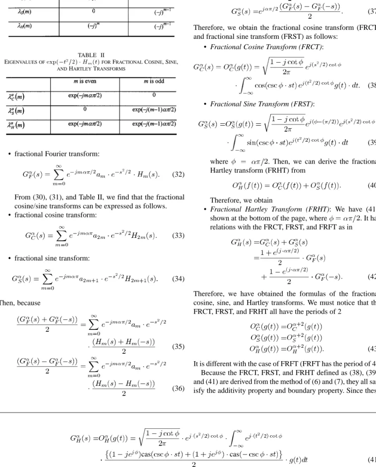
Their corresponding eigenvalues (which are denoted by ) are shown in Table I.
We can derive fractional cosine, sine, and Hartley transforms from the method of (6) and (7). Similar to the derivation process of the fractional Fourier transform (FRFT) introduced in [3] (which is listed in (10)–(14)), we can derive these fractional transforms from the process as follows.
1) where is defined as (11) (29) 2) (30) 3) (31)
where is the fractional power of
eigen-values of cosine, sine, and Hartley transforms, as shown in Table II.
From (13) and (14), we can express the FRFT as follows
TABLE I
EIGENVALUES OFexp(0t =2) 1 H (t)FORCOSINE, SINE,
ANDHARTLEYTRANSFORMS
TABLE II
EIGENVALUES OFexp(0t =2) 1 H (t)FORFRACTIONALCOSINE, SINE,
ANDHARTLEYTRANSFORMS
• fractional Fourier transform:
(32)
From (30), (31), and Table II, we find that the fractional cosine/sine transforms can be expressed as follows. • fractional cosine transform:
(33)
• fractional sine transform:
(34)
Then, because
(35)
(36)
and is even when is even, is odd when
is odd; therefore, we find the fractional cosine/sine transforms have the following relations with the FRFT:
(37) Therefore, we obtain the fractional cosine transform (FRCT) and fractional sine transform (FRST) as follows:
• Fractional Cosine Transform (FRCT):
(38) • Fractional Sine Transform (FRST):
(39)
where . Then, we can derive the fractional
Hartley transform (FRHT) from
(40) Therefore, we obtain
• Fractional Hartley Transform (FRHT): We have (41), shown at the bottom of the page, where . It has relations with the FRCT, FRST, and FRFT as in
(42) Therefore, we have obtained the formulas of the fractional cosine, sine, and Hartley transforms. We must notice that the FRCT, FRST, and FRHT all have the periods of 2
(43) It is different with the case of FRFT (FRFT has the period of 4). Because the FRCT, FRST, and FRHT defined as (38), (39), and (41) are derived from the method of (6) and (7), they all sat-isfy the additivity property and boundary property. Since these
cas cas
fractional transforms have the additivity property, they are all reversible, and their inverse transforms are
if is even
if is odd (44)
no matter
whether is even or odd (45)
The FRCT has no odd eigenfunctions, and the FRST has no even eigenfunctions. Thus, as the original cosine and sine trans-forms, the odd part of input function will be lost after doing the FRCT, and the even part of input will be lost after doing the FRST. Therefore, it is better to use the FRCT to process even functions and use the FRST to process odd functions. There-fore, we can constrain the input function of FRCT to be even and define the one-sided FRCT as follows.
• One-sided fractional cosine transform (One-sided FRCT):
(46) We can constrain the input function of FRST to be odd and define the one-sided FRST as follows.
• One-side fractional sine transform (One-sided FRST):
(47) We notice that the transform results of the one-sided FRCT/FRST are the same as the transform results of FRFT for even/odd functions
when is even
when is odd (48)
When we use the one-sided FRCT/FRST to process the even/odd functions, the complexity of computation is half of the complexity of the FRFT (because the range of integration for the one-sided FRCT, FRST is . Therefore, the one-sided FRCT/FRSTs are more efficient than the FRFT when processing the even/odd functions.
III. CANONICALCOSINE ANDSINETRANSFORMS
A. Linear Canonical Transform and its Eigenfunctions
Canonical cosine and sine transforms are the further gener-alization of FRCT and FRST. They are analogous to the linear
canonical transform (LCT) [2], [13], [14]. The LCT is the
gen-eralization of the FRFT [see (9)]. It is defined as
for (49)
TABLE III
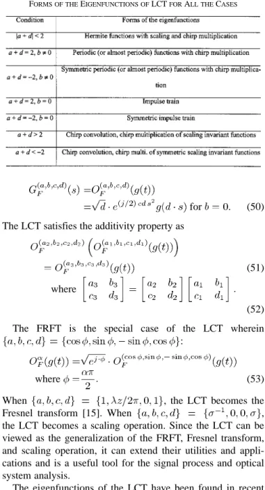
FORMS OF THEEIGENFUNCTIONS OFLCTFORALL THECASES
for (50)
The LCT satisfies the additivity property as
(51) where
(52) The FRFT is the special case of the LCT wherein
:
where (53)
When , the LCT becomes the
Fresnel transform [15]. When ,
the LCT becomes a scaling operation. Since the LCT can be viewed as the generalization of the FRFT, Fresnel transform, and scaling operation, it can extend their utilities and appli-cations and is a useful tool for the signal process and optical system analysis.
The eigenfunctions of the LCT have been found in recent years [16], [17]. Since listing the explicit formulas of the eigen-functions of the LCT for each case is too complicated, we just list their forms in Table III. The details about the eigenfunctions of the LCT are described in [17].
For different cases, the forms of the eigenfunctions are also different. Nevertheless, in all cases, the eigenfunctions of the LCT all have the properties of orthogonality, completion, and symmetry properties of the eigenfunctions of LCT.
There is at least one subset of the eigenfunctions of the LCT with parameters that forms an orthogonal, complete,
and symmetric function set. That is, we can always find an
eigenfunctions set of the LCT with
parameters that satisfies the following. 1)
2) Any function can be expressed as the linear combi-nation of
where (55)
3) are either symmetric or
asymmetric
or (56)
That is, is either even or odd.
This property is very helpful for us to derive canonical cosine and sine transforms from the LCT.
B. Deriving the Canonical Cosine and Sine Transforms
From the above property, we know that for the LCT
with any parameters set , we can always find an
orthogonal, complete, and symmetric eigenfunctions set . Since the eigenfunctions set is complete and symmetric, we can sort the eigenfunctions set
properly so that is even and is odd
(57) Since the eigenfunctions set is orthogonal and complete, as is the case of the FRFT, we can express the LCT as the following process instead of (50) and (51).
1)
(58) 2)
where is the eigenvalue of the LCT for
(59) 3)
(60)
Then, we try to define the canonical cosine transform (CCT) with parameters . As with the case of the fractional cosine transform (FRCT), we choose the eigenfunctions of the CCT with parameters as the even eigenfunctions of
the LCT with parameters , and the corresponding
eigenvalues are the same. We also set the odd eigenfunctions of the LCT with parameters to belong to the null space
of the LCT with parameters :
(61)
Similarly, for the canonical sine transform (CST) with
parame-ters , we choose
(62) The CCT and CST can be expressed as the following process.
1)
where are defined as (58). (63)
2)
where is the eigenvalue of the LCT for (64) 3)
(65)
The only difference among the CCT, CST, and LCT is the last step. Since
(66) and
(67) The formulas of the canonical cosine and sine transforms we derived are as follows.
• Canonical Cosine Transform (CCT):
for (68)
• Canonical Sine Transform (CST):
for (70)
for (71)
The FRCT/FRST derived in Section II are the special cases of the CCT/CST where
(with the difference of some constant phase) (72)
where (73)
The CCT and CST have additivity property as follows.
if is even (74)
if is odd (75)
where (76)
We can now prove them.
(Proof of the additivity properties of CCT and CST): Since
(77)
from (66), we obtain
(78) where we have (78a), shown at the bottom of the page. Then, we use the additivity property of LCT and obtain (79), shown at the bottom of the page. Therefore, we have proved the additivity property of CCT (74). We can use similar process to prove the additivity property of CST (75).
Since CCT and CST are all additive, they are all reversible, and the inverse operations of the CCT and CST with
param-eters is just the CCT and CST with parameters
if is even (80)
if is odd (81)
Although we can define the CCT and CST, the canonical Hartley transform (CHT) is very hard to define. We cannot de-fine it as the summation of the CCT and the CST because the re-sult has no additivity property. It is also hard to apply the method as Figs. 1 and 2. Nevertheless, since the original Hartley trans-form has the relation with the FT as
(82) we suggest that we can define the CHT as
(83) We can prove that the CHT defined above has an additivity prop-erty, but the FRHT defined in Section II is not its special case.
(78a)
C. One-Sided Canonical Cosine, Sine Transforms
We can prove that for even/odd inputs, the transform results of the CCT/CST are the same as the transform results of the linear canonical transform (LCT)
if is even (84)
if is odd (85)
As with the case of the FRCT and FRST, the CCT is suitable to deal with the even functions, and the CST is suitable to deal with the odd functions. We can constrain the input function of the CCT to be even and constrain the input function of the CST to be odd and define the one-sided CCT and the one-sided CST as follows.
• One-sided canonical cosine transform (one-sided CCT)
for (86)
for (87)
• One-sided canonical sine transform (one-sided CST)
for (88)
for (89)
Since the range of integration for the one-sided CCT/CST is
just and not , using the one-sided CCT/CST
is more efficient than using the LCT to deal with the even/odd functions.
IV. SIMPLIFIEDFRCT, FRST,ANDFRHTS
The FRCT, FRST, FRHT, CCT, and CST derived in Sections II and III all have the additivity property and are suitable to deal with the even and odd functions. Nevertheless, for real input, the transform results of these transforms are not real. The original FRCT, FRST, and FRHTs are suitable to deal with the real functions because for real input, the output is also real. This advantage does not exist for the transforms derived in Sections II and III.
In this section, we will derive the SFRCT, SFRST, and SFRHTs. Their performances are very similar to those of the FRCT, FRST, and FRHT and have the advantage of real-input–real-output.
A. Review of SFRFT
Before discussing the SFRCT, SFRST, and SFRHT, we first describe the SFRFT. It was introduced in [19] recently. In [19], we had illustrated that although the LCT has four parameters , in many applications, only the value of really effects the performance. Therefore, if , then the
LCT with parameters will have the same effects
as the LCT with parameters for many
applica-tions (such as filter design).
We remember that the FRFT is a special case of the LCT
where .
Therefore, for the FRFT, the value of is . Thus, we can define the SFRFT as the special case of the LCT where ; then, it will have the same effects as the FRFT. Then, we choose other parameters properly such that the SFRFT will be simpler than the FRFT for digital implementa-tion, optical system implementaimplementa-tion, gradient-index medium implementation, etc. In [19], we defined several types of SFRFT. The most important one is the following.
• SFRFT:
where (90)
It is the special case of the LCT with parameters . It has the same effects as the FRFT and has two important advantages.
1) Compared with the original FRFT [see (9)], for the SFRFT defined as (90), the outer chirp term is re-moved, and the complexity of design and computa-tion is reduced.
2) Suppose that and are the sampling intervals in time and frequency domains. For the case of FRFT,
if we try to make the term in (9)
become the kernel of the DFT, then
(91) Since varies with , we must adjust the value of or when is changed, but for the SFRFT,
to make the term in (90) become the
kernel of the DFT, we just have to set
(92) This does not vary with , and we do not have to adjust the value of and when is changed. Therefore, for digital implementation, the SFRFT defined as (90) is simpler than the original FRFT. It can substitute the FRFT for many applications.
B. SFRCT
We will derive the SFRCT. The SFRCT we derive should have at least the two advantages: i) It is efficient for digital implementation, and ii) for real input, the output is also real.
We will try to achieve these two goals. The SFRFT with pa-rameter is the special case of the LCT where
. For the CCT [see (68)], when , then
(93) We can define the SFRCT as (we suppose that the input is a real function)
Re
(94) Since, as with the FRCT and CCT we will usually use the SFRCT to process even function, in (94), it is convenient to
change the range of integration from into .
Therefore, we obtain the following. • SFRCT of type 1:
where (95)
The SFRCT has very close relation with the SFRFT, especially when the input is a real, even function. We now prove this statement. Suppose is a real, even function. From the even-input–even-output property of the SFRFT:
if (96)
we can conclude that , and hence , are
all even functions. Therefore
Re Re
Re Re
Re
Re
(97) Thus, if the input is a real, even function, then the trans-form result of the SFRCT is the same as the real part of , where is the transform result of the SFRFT. Therefore, the SFRCT has a very close relation with the SFRFT, especially when the input is real and even.
We remember that if the input function is a real, even function, then the transform result of the original cosine transform is the same as the transform result of the FT. This means that the original cosine transform is suitable to deal with the real, even functions. Similarly, from the relation of (97), we can conclude that the SFRCT is also suitable to deal with the real, even functions. Suppose, for digital implementation, that the sampling points of the input function are
(98) Then, in the case where is real and even, we just have to store the values of
Re (99)
and there are only real values to store. For the SFRFT of , because the transform result is usually a complex, even function, we must store the values of
Re Im
(100) and there are real values to store (twice of the input). It is overdetermined and wastes the storage and computation time. In contrast, for the case of SFRCT, we just have to store
Re (101)
and there are totally real values to store (the same as the input). It is very reasonable that the storage required for the transform result is the same as the storage required for the input because it means no information loss and no redundancy. Since the degree of freedom is halved, using the SFRCT to deal with the real, even functions is more efficient than using the SFRFT.
In Section IV-A, we have stated for digital implementa-tion that the SFRFT is more efficient than the FRFT. Here, we have proved that the SFRCT is even more efficient than the SFRFT if the input is real and even. Using the SFRCT to process the real, even functions is better than using the SFRFT, and hence, it is better than using the FRFT.
The SFRCT defined as (95) has no additivity property. In mathematics, it does not do as well as the FRCT intro-duced in Section II. We derived the SFRCT mainly from the consideration of practical applications. Although the SFRCT has no additivity property, it is still easy to recover the original function from the transform result.
• Inverse SFRCT of type 1:
where (102)
In (102), it is possible that for some
, but this problem is not important for the digital imple-mentation because we can choose the sampling interval
The SFRCT we defined in (95) is similar to the FRCT defined by [9] [which is shown in (19)]. They all have the property of real-input–real-output, and all have no addi-tivity property. Nevertheless, there are two key differences between them. The first difference is that it is easy to re-cover the original function from the transform result of SFRCT [just using (102)], but for the FRCT defined as (19), we must follow the complicated process from (23) to (25) to recover the original function.
The second difference is about the digital computation. For the FRCT defined as (19), we must implement it by the FRFT. For the SFRCT defined as (95), we can imple-ment it without resorting to the FRFT. We can use a more efficient algorithm, such as applying the fast algorithm of the DCT, and the complexity of computation can be much less (see Section VI).
In fact, there are also other types of the SFRCT. In (94), we define the SFRCT as the real part of . We can also take its imagi-nary part and define the SFRCT of type 2 as follows. • SFRCT of type 2:
where (103)
Its inverse transform is
(104) We can prove
Im
if the input is real and even (105) As in the case of the SFRCT of type 1, the SFRCT of type 2 also has a very close relation with the SFRFT when the input is a real, even function. The SFRCT of type 1 preserves the real part of , and the SFRCT of type 2 preserves its imaginary part. They all treat the other part as the redundancy and make the degree of freedom of the transform result the same as that of the input when the input is a real, even function. They can deal with real, even functions more efficiently than the SFRFT and the FRFT.
C. SFRST and SFRHTs
As with the SFRCT, we can define the SFRST from the CST
with parameters and take the real/imaginary
parts
Re (106)
We also suppose the input is a real, odd function. Then together, with (70), we obtain the following.
• SFRST of type 1:
where (107)
• SFRST of type 2:
where (108)
In addition, their inverse transforms are
(109)
(110) Thus, although the SFRST has no additivity property, from (109) and (110), it is still easy to recover the original function from the transform result of the SFRST.
We can prove that if is a real, odd function, then the transform results of the SFRFT of type 1 and type 2 and the transform result of the SFRST will have the relation
Re
Im (111)
when is a real, odd function. The transform result of the SFRFT is real if the input is a real function. In contrast, the transform results of the SFRFT and FRFT are complex even when the input is real. Therefore, when processing the real, odd functions, we can use the SFRST instead of the SFRFT and FRFT to improve the efficiency.
Then, we try to define the SFRHT. Since the original Hartley transform is the summation of the original cosine and sine trans-forms, we can also define the SFRHT by a similar way. We de-fine the SFRHT of type 1 as the summation of the SFRCT of type 1 and the SFRST of type 2 (since they all have the term of ) and define the SFRHT of type 2 as the sum-mation of the SFRCT of type 2 and the SFRST of type 1
(112) We thus have the following.
• SFRHT of type 1: cas where (113) • SFRHT of type 2: cas where (114)
Here, we change the range of integration from back into since we no longer constrain the input to be even or odd. The inverse transforms of the SFRHT of types 1 and 2 are
cas (115)
cas (116)
If the input function is real, then the transform results of the SFRHT of types 1 and 2 and the transform result of the SFRFT will have the relations such as
Re Even Im Odd when is real Im Even Re Odd when is real (117)
Therefore, the SFRHT has very close relation with the SFRFT. The SFRHT has the advantage of real-input–real-output. In con-trast, the SFRFT and FRFT do not have this advantage and re-quire more storage and more computation time to process the real functions. Therefore, when dealing with the real functions, it is more efficient to use the SFRHT instead of the SFRFT and FRFT.
In summary, the advantages of the SFRCT, SFRST, and SFRHT are the following.
1) For the real input, the output is also a real function. Sim-ilarly, for the pure imaginary input, the output is also a pure imaginary function.
2) The amount of required storage can be saved. When we use the SFRCT, SFRST, and SFRHT to deal with pure real/imaginary functions, the amount of storage required is only half of the storage required for SFRFT and FRFT. 3) It is easy to recover the original function from the
trans-form results of the SFRCT, SFRST, and SFRHT. This
ad-vantage is very important for the applications; we must do both the forward and the inverse transforms (such as filter design).
4) They are very efficient for digital implementation. In Section VI, we will show, with the aid of the fast algo-rithm of the DCT, DST, and DHT, that the complexities of digital implementation of the SFRCT, SFRST, and SFRHT are much less than those of the FRCT, FRST, FRHT, which are defined as (19) and (21). They are also more efficient than all the fractional and canonical transforms introduced in Sections II and III for digital implementation, especially for real input functions.
V. PROPERTIES
In this section, we will discuss the properties of the CCT and SFRCT. Most properties of the FRCT can be obtained from the properties of the CCT by substituting as
, where . The properties of the
FRST, FRHT, and CST are similar to the properties of the FRCT and CCT. The properties of the SFRST and SFRHT are similar to the properties of the SFRCT.
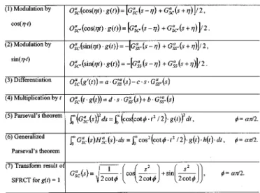
We first list the properties of the CCT in Table IV.
Although the properties in Table IV are derived for the two-sided CCT, if we constrain the input function of the one-two-sided CCT to be even, then these properties can also be applied to the one-sided CCT defined as (86). We notice that for some properties of the CCT, such as the differentiation property, we cannot just use the CCT to describe it. We must describe them by the CST. In Table IV, Properties 5 and 6 can be combined as
(118)
where
(119)
Therefore, the differentiation-multiplication operations pair has a very close relation with the CCT.
Then, we list the properties of the SFRCT in Table V ( means the SFRCT of type 1, and means the SFRCT of type 2). In Properties 1, 5, and 6, the input function is con-strained to be real and even, and in Properties 2–4, the input is constrained to be real and odd.
We notice that the modulation property (Properties 1 and 2) of the SFRCT is independent of . If we multiply the input
func-tion by or , then whatever the value of is, in
frequency domain, it will always cause the displacement of . For the case of the CCT and FRCT, from Properties 3 and 4 in
TABLE IV PROPERTIES OF THECCT
Table IV, the amount of displacement depends on their parame-ters. The fact that the modulation property is independent of is also an advantage of the SFRCT.
VI. DIGITALIMPLEMENTATION
A. Review of the Digital Implementation of the FRFT, LCT, and SFRFT
In this section, we will discuss the digital implementation methods of all the fractional, canonical, and simplified frac-tional transforms introduced in Section II–IV. For the conve-nience of comparison, we first review the digital implementa-tion of the FRFT, LCT, and SFRFT.
In [12] and [29], the authors stated that we require two -point multiplications ( is the total number of sampling points) and one -points convolution to implement the FRFT
TABLE V PROPERTIES OF THESFRCT
or LCT. Then, in our paper [28], we have stated that we can constrain the sampling intervals in the time and frequency domains to satisfy
for FRFT for LCT
(120) In this case, we just require two chirp multiplications and one DFT to implement the FRFT or LCT. Since the DFT requires complex multiplications (using the split-radix
algorithm), we totally require complex
mul-tiplications to implement the FRFT or LCT if (120) is satisfied. Because each complex number multiplication requires three real number multiplications, the amount of real number multiplica-tions required for the FRFT or LCT is
(121) The SFRFT is the special case of the LCT where , and therefore, its com-plexity is similar to the comcom-plexity of the LCT, except that one chirp multiplication can be saved (since ). Therefore, the amount of real number multiplications required for the SFRFT is
(if the sampling intervals satisfy (122)
B. Using the Fast Algorithm of FRFT or LCT
We now discuss the digital implementation of all the trans-forms introduced in Sections II–IV. We can apply the fast al-gorithms of the DCT [20]–[23], [25], [27], DST [22], [23], and DHT [10], [24], [26] to implement these transforms.
We first discuss how to use DCT to implement the FRCT. We can first sample the -axis and -axis as
Then, together with the formula of the one-sided FRCT ((46)), we can implement the FRCT as
(124)
Then, we choose the values of , , , and properly to make the cosine term in (124) becomes the kernel of the DCT, and we can use the fast algorithm of the DCT [20]–[23], [25], [27] together with the chirp multiplications to implement the FRCT. The amount of real number multiplications required for the DCT, when the input is a real function, is [20], [27] as follows.
• For the first-type DCT
(125)
• For the second- and the third-type DCT
(126)
• For the fourth-type DCT
(127)
They are much less than the amount of real number multiplica-tions required for the DFT (about ). Therefore, if we implement the FRCT by the DCT, then the complexity of the FRCT will be much less than the complexity of the FRFT (be-cause the FRFT is implemented by the DFT).
For example, if we choose , , , and as
(128)
then (124) becomes
(129)
where
for (130)
We notice that is just the kernel of the
first-type DCT. Therefore, in this case, we can use the fast al-gorithm of the first-type DCT to implement the FRCT. We can follow the process as follows.
1) Do the chirp multiplication as (130) to obtain . 2) Then, do the first-type DCT for .
3) Then, multiply the above transform result by the outside chirp term, as (129).
The first and the third steps both require -point complex mul-tiplication (i.e., real multiplications). Since, for the second step, the input is a complex function, we do the first-type DCT with real input function twice, and the real number multiplica-tions required for the second step is twice (125) Thus, the total amount of real number multiplications required is
(131) Since, from (123), is just the number of sampling points for , if is the total number of sampling points (including the
sampling points for and ), then .
Therefore, (131) can be rewritten as follows.
• Amount of the real multiplications required for the FRCT
implemented by the first-type DCT:
(132)
We can compare this with the complexity of the FRFT [see (121)]. The complexity of the FRCT is just about half of the complexity of the FRFT. When we deal with the even functions, it is much more efficient to use the FRCT than to use the original FRFT. The FRCT is really an efficient tool to process the even functions.
Except for the first-type DCT, we can also use the second-, the third-, and the fourth-type DCTs to implement the FRCT. In these cases, we choose the values of , , , and in (124) as
for the second-type DCT for the third-type DCT
for the fourth-type DCT
In these cases, the amount of real multiplications required for the FRCT are also about half of the amount of real number mul-tiplications required for the FRFT.
Similarly, we can also implement the CCT by the DCT, and the number of multiplications required is also the same as or near (132). It is about half of the amount of real number multi-plications required for the LCT.
C. Using DST and DHT to Implement the FRST, FRHT, and CST
Similarly, we can use the fast algorithm of the DST [22], [23] to implement the FRST and CST and use the fast algorithm of the DHT [10], [24], [26] to implement the FRHT.
We can implement the FRST and CST by two chirp cations and one DST. Since the amount of real number multipli-cations required for the DST is about
(when the input of the DST is a real function) (133) the total amounts of real multiplications required for the FRST and CST are about
(134)
where is the total number of sampling points, and
is the number of sampling points for . (It is also the length of the input function of DST.)
We can also use two chirp multiplications and one DHT to implement the FRHT. The amount of real number multiplica-tions required for the DHT is about
(135)
For the case of the DHT, since the input function is neither even nor odd, the number of points of the input function of the DHT must equal the total number of sampling points, i.e., . The total amount of real number multiplications required for the FRHT is
(136)
Comparing (134) with (121), we find the complexities of the FRST and CST to be only half of the complexities of the FRFT and LCT. It is quite efficient to use the FRST/CST instead of the FRFT/LCT to process odd functions. Besides, the FRHT is also an efficient signal processing tool.
D. Implementation of the SFRCT, SFRST, and SFRHT
For the SFRCT of type 1, we can sample the and axes as (123). Then, (95) becomes
(137)
When we choose , , , and properly, then the cosine term of the above equation becomes the kernel of the DCT of type 1, 2, 3, or 4, and we can use the fast algorithm of the DCT of type 1, 2, 3, or 4 to implement it. For example, if we choose
, , , and as
(138) then (138) becomes
where (139)
for (140)
Then, we can implement the SFRCT of type 1 by the first-type
DCT together with the multiplication of .
Since the input function of the SFRCT is constrained to be a real function, (140) is the multiplication operation be-tween two real functions. It requires real number multipli-cations because if is real, then the input of the first-type DCT is also a real function, and the amount of real multiplications required for the first-type DCT with real input
is . Therefore, he total amount of real
number multiplications required for the SFRCT implemented by the first-type DCT is as follows.
• Amount of real multiplications required for the SFRCT
implemented by the first-type DCT
(141)
We also use the fact that (the length of the input for DCT, i.e., the number of sampling points for ) is about half of (the total number of sampling points) for the case of the SFRCT. Equation (141) is not only much less than the complexities of the FRFT and LCT [see (121)] (about one fourth) but is also less than the complexities of the FRCT and CCT [see (132)] (about one half). When the input function is both real and even, it is much more efficient to use the SFRCT to process it than to use the FRFT, LCT, FRCT, and CCT.
In (138), the product of sampling intervals , is fixed to . It is independent of the parameter of SFRCT. We do not have to adjust , when is changed. This advantage does not exist for the FRCT and CCT.
We can use a similar algorithm to implement the SFRCT of type 2.
By the same reasons, we can use the fast algorithms of the DST and DHT to implement the SFRST and SFRHT of types 1
and 2. We require one multiplication of [or
] and one DST (or DHT) to implement these
transforms. Since or
is the multiplication operation between two real functions, and the input of DST is a real function, the
total amount of real multiplications required for the SFRST (no matter for type 1 or type 2) implemented by the DST is
(142) Similarly, the total amount of real multiplications required for the SFRHT (no matter for type 1 or type 2) implemented by the DHT is
(143)
We remember that for the case of the SFRST, , and for the case of the SFRHT, .
Comparing (142) and (143) with (121), (134), and (136), we find that the complexity of the SFRST is one fourth of the com-plexities of the FRFT or LCT and is one half of the complexity of FRST or CST. The complexity of SFRHT is one half of the complexities of FRFT or LCT, and FRHT. Therefore, it is much more efficient to use the SFRST to deal with the real, odd func-tions than using other transforms. It is also more efficient to use the SFRHT to deal with pure real/imaginary functions than to use other transforms.
VII. APPLICATIONS
A. Substituting the FRFT and LCT
The transforms introduced in this paper have an important advantage. That is, they can replace the FRFT and LCT when the input function is even, odd, pure real, or pure imaginary. From Sections II–IV, we have known that the FRCT and FRST have very close relations with the the FRFT. The CCT and CST have very close relations with the LCT. The SFRCT, SFRST, and SFRHT have very close relations with the SFRST and, hence, the FRFT. Therefore, the performances of these transforms are very similar to the performances of the FRFT and LCT.
In Section VI, we have stated the following.
1) When we use the FRCT and CCT to process even
func-tions, then the amount of the required real number
multi-plications is only one half of those of the FRFT and LCT. 2) When we use the FRST and CST to process odd functions, then the amount of the required real number multiplica-tions is only one half of those of the FRFT and LCT. 3) When we use the SFRHT to process pure real/imaginary
functions, then the amount of the required real number
multiplications is only one half of those of the FRFT and LCT.
4) When we use the SFRCT to process pure
real/imagi-nary, even functions, then the amount of the required real
number multiplications is only one fourth of those of the FRFT and LCT.
5) When we use the SFRST to process pure real/imaginary,
odd functions, then the amount of the required real
number multiplications is only one fourth of those of the FRFT and LCT.
Since the performances of the FRCT, FRST, CCT, CST, SFRCT, SFRST, and SFRHT are similar to the performances of the FRFT, LCT, and SFRFT and their complexities are much
less, we can use these transforms to replace the the FRFT and LCT if the input is even, odd, pure real, or pure imaginary.
Thus, all the applications of the FRFT and LCT are also the
applications of the transforms introduced in this paper. The
ap-plications of the FRFT and LCT are filter design, optical system analysis, radar system analysis, solving differential equations, phase retrieval, multiplexing, space-variant pattern recognition, localized edge detection, etc. They will also be the applications of the transforms introduced in this paper. In Sections VII-A1–3, we give three examples:
1) optical system analysis, 2) filter design,
3) pattern recognition.
They are all the applications of the FRFT and LCT and, hence, the applications of the transforms introduced in this paper.
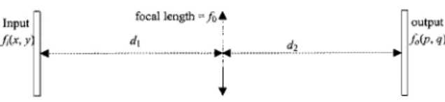
1) Optical System Analysis: For the optical system as
Fig. 3, the relation between the input and output can be expressed as the LCT with parameters
, where [19]
(144) where
is some constant phase
(the kernel of LCT) (145)
In the case that the input is even for both the and axes (146) then we can use the CCT with the same parameters to substitute the LCT for both and -axes, and change (144) to be
(147) where the values of are the same as (145), is some
constant phase, and is the kernel of the
one-sided CCT
(148) The value of calculated from (147) is the same as the value of calculated from (144), but since the complexity of the CCT is about one half of the complexity of the LCT, the complexity of (147) is just about one fourth of the complexity of (144).
Similarly, if the input is even for the axis and odd for the axis
Fig. 3. Optical system with one spherical lens and two free spaces.
then in (144), we can use the CCT instead of the LCT for the axis and use the CST instead of the LCT for the axis. When the input is odd for the axis and even for the axis, we can use the CST for the axis and use the CCT for the axis. When the input is odd for both the axis and axis, we can also use the CST for both the axis and the axis. For all of these cases, the complexities of computation are just about one fourth of the complexity when we use the LCT directly.
For the application of optical system analysis, we can use CCT and CST instead of the LCT to improve the efficiency when the input is even or odd.
2) Filter Design: The filter designed by the FRFT [18] can
be expressed as
(150) where is the received signal. We try to design the proper values of and such that the output is near the orig-inal signal. This type of filter is more flexible and can do more things than the filter designed by the FT.
Since, in practice, the received signal is usually a real function, in (150), it may be convenient to use the SFRHT in-stead of the FRFT
(151) From Section VI-D, the complexity of the SFRHT is just about one half of the complexity of the FRFT; for the real signal, using the SFRHT for filter design is more efficient than using the FRFT.
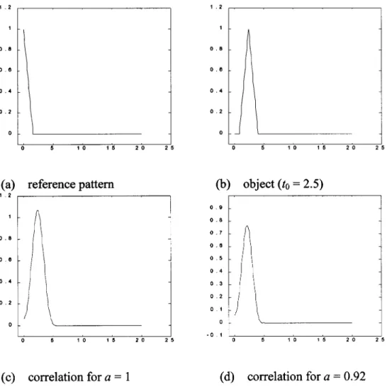
3) Application of the SFRCT for Space-Variant Pattern Recognition: In [6], the authors found, with the aid of
frac-tional correlation, that the FRFT can be used for space variant pattern recognition. Fractional correlation [30] is defined as
(152) For the application of space-variant pattern recognition, we treat as the reference pattern and treat as the input object. Then, we calculate and find the peak value of . If
Max threshold (153)
then we conclude that the input object matches the reference pattern and that the location difference between the input object and the reference pattern is within some certain region. That is
and (154)
If the input object does not match the reference pattern or the lo-cation difference is too large, then (153) will not be satisfied, and the input object will not be recognized as matching the reference
pattern. Therefore, it is called space-variant pattern recognition. The value of in (154) is affected by . If, in (152), we set , i.e., we do the original FTs for and , then the value of will be infinite. If we choose the value of between 0 and 1, then the value of will be finite. When the value of
is smaller, then the value of is also smaller. Because, for the application of space-variant pattern recogni-tion, the reference pattern and the input object are always real functions, we can use the SFRCT, SFRST, and SFRHT instead of the the FRFTs in (152) to improve efficiency.
For example, we can use the SFRCTs instead of the FRFTs in (152) when the reference pattern is a real, even function. Due to the displacement, the input object is always not an even function, but from our experiments, it does not cause any problem when we replace all the FRFTs with SFRCTs. We just require the reference pattern to be a real, even function. If we use SFRCTs instead of FRFTs in (152), then (152) is changed as
(155) where means the original cosine transform. We call (155) the FRCCR of and . We notice that (155) can be rewritten as
where
If is the displacement of , as (157), then after some computation, we can prove that the maximum of usually occurs at the location of , and its value is
Max
(156) where . Therefore, we conclude that the value of Max is affected by whether the input object matches the reference pattern and whether the displacement is sufficient small. For a fixed value of , Max is large when is small, and Max is small when is large. The value
of can control how fast Max varies with . If is
larger, then Max will decay faster with . Therefore, if we want (153) to be satisfied, then the input object must match the reference pattern , and their location difference should not be very large:
Fig. 4. Space-variant pattern recognition. (a) Referencex(t). (b) Input y(t) = x(t 0 3). (c) Result (absolute value) of FRCCR with a = 1. (d) Result (absolute value) of FRCCR witha = 0:9.
The value of is affected by . If is smaller,
then is also smaller. Therefore, we can use the SFRCT for space-variant pattern recognition when the reference pattern is real] and even.
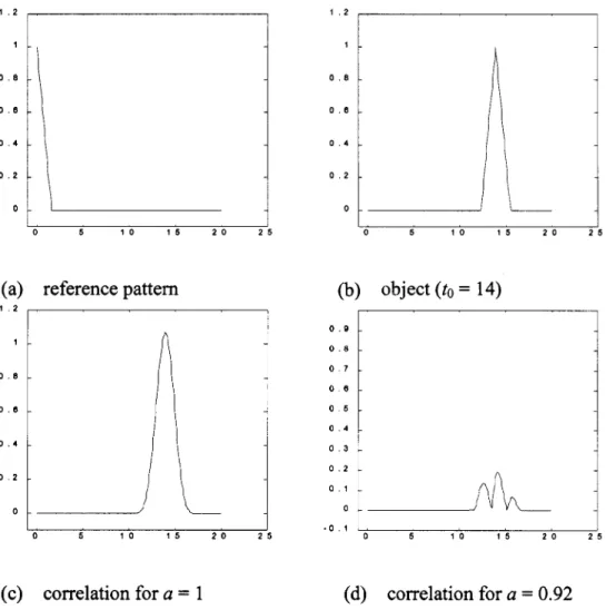
We give an example in the following. Here, we choose the reference pattern as a triangular function
(158) We plot for in Figs. 4(a) and 5(a). Then, we choose the input object as
for Fig4:
for Fig5: (159)
They are plotted in Figs. 4(b) and 5(b). They all match the ref-erence pattern but have different amount of displacement. Then, we do the FRCCR with [in this case, the SFRCTs in (155) all become the original cosine transforms] for and and plot the results in Figs. 4(c) and 5(c). Finally, we do the FRCCR
with for and and plot the results in Figs. 4(d)
and 5(d).
From the above experiments, we find, for the case that , that the value of Max ( is the output of FRCCR) is al-most independent of . This is because in this case, the value of in (156) equals to 0; therefore, has no effect
on the value of Max . For the case where , from
Figs. 4(d) and 5(d), we find that the value of Max decreases with . In this case, we can choose the threshold properly such that only when is within some region, the value of Max will be above the threshold. Therefore, we can use the SFRCT for space-variant pattern recognition when and when the reference pattern is real and even.
B. One-Sided Signal Processing and Other Potential Applications
In Section VII-A, we have stated that we can use the trans-forms introduced in this paper to substitute the FRFT and LCT in many conditions. In fact, except for substituting the FRFT and LCT, there are also other potential applications for these transforms.
We can use the FRCT, FTST, CCT, CST, FRSCT, and FRSST for one-sided signal processing. For one-sided signal processing, the time interval we considered is
Fig. 5. Space-variant pattern recognition. (a) Referencex(t). (b) Input y(t) = x(t 0 14). (c) Result (absolute value) of FRCCR with a = 1. (d) Result (absolute value) of FRCCR witha = 0:9.
In this case, the constraint of the one-sided FRCT to be re-versible is
where is the input of the one-sided FRCT (161) This is also the constraint that we can use the FRCT for one-sided signal processing.
Proof of (161): If is reversible after doing the one-sided FRCT, then it can be expressed as
(162) Then, because
if is reversible after doing the one-sided FRCT, then must be satisfied.
Similarly, is also the constraint for the one-sided CCT [see (86) and (87)] and the SFRCT [(95) and (103)] to be reversible
if (163)
If the input function has zero differential value at , then we can use the one-sided FRCT, one-sided CCT, and the SFRCT for one-sided signal processing.
Similarly, we can also conclude that for one-sided signal pro-cessing, if the input satisfies
(164) then it is reversible for one-sided FRST, one-sided CST, and the SFRST. We can use these transforms for one-sided signal processing when the initial value of the input is zero.
If the input function satisfies or , then we
can use the generalized cosine and sine transforms introduced in this paper for one-sided signal processing. We can use them to solve the differential equations with zero initial value or zero ini-tial differenini-tial value. We can also use them for one-sided filter
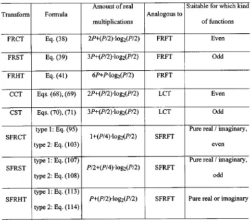
TABLE VI
SUMMARY OF THEFRACTIONAL, CANONICAL,ANDSIMPLIFIEDCOSINE, SINE,
ANDHARTLEYTRANSFORMSINTRODUCED INTHISPAPER
design and other applications. Although the conventional cosine and sine transforms can also be used for one-sided signal pro-cessing, using the family of generalized cosine and sine trans-forms can solve more problems. For example, for the noise (we notice that it has zero differential value at )
for (165)
it is hard to use the conventional one-sided cosine transform to remove it. In contrast, if we use the one-sided FRCT or CCT, then we can remove the above noise easily.
In fact, if and , then we can still use
the FRCT, FRST, CCT, CST, SFRCT, and SFRST for one-sided signal processing, but in this case, there are some errors around
.
Although the family of generalized Hartley transforms cannot be used for one-sided signal processing, they also have some po-tential applications. For example, since the performance and the efficiency of FRHT is near those of the FRFT, for the consider-ation of encryption, we can use the FRHT instead of the FRFT. Besides, for the SFRHT introduced in Section IV-C, except for substituting the FRFT and LCT when processing a real signal, it is also useful to deal with the signal that is the linear combi-nation of
cas
is some fixed constant (166) or
cas
is some fixed constant (167)
VIII. CONCLUSION
In this paper, we have derived the fractional, canonical, and simplified fractional cosine, sine, and Hartley transforms. They are the generalization of the original cosine, sine, and Hartley
transforms. We also discuss their properties, digital implemen-tation, and applications. We summarize all the transforms de-rived in this paper in Table VI.
The original cosine, sine, and Hartley transforms can replace the FT when we deal with the even, odd, and pure real/imag-inary functions. Similarly, among the transforms derived in paper, the FRCT and CCT can replace the FRFT and LCT when we deal with even functions. The FRST and CST can replace the FRFT and LCT when we deal with odd functions. The SFRHT can replace the FRFT and LCT when we deal with pure real/imaginary functions. The SFRCT is suitable for processing pure real/imaginary, even functions, and the SFRST is suitable for processing pure real/imaginary, odd functions. From the discussion in Section VI, the complexities of these transforms are much less than the complexities of the FRFT and LCT. We can just use one half or one fourth of the real number multiplications required for the FRFT and LCT to implement these transforms.
The FRFT and LCT are useful signal processing tools. Since the transforms derived in this paper can be substituted for the FRFT and LCT under many conditions, we believe they will also become useful signal processing tools in the future.
REFERENCES
[1] M. R. Spiegel, Mathematical Handbook of Formulas and Tables. New York: McGraw-Hill, 1990.
[2] N. Wiener, “Hermitian polynomials and fourier analysis,” MIT J. Math.
Phys., vol. 18, pp. 70–73, 1929.
[3] V. Namias, “The fractional order Fourier transform and its application to quantum mechanics,” J. Inst. Math. Appl., vol. 25, pp. 241–265, 1980. [4] P. M. Morse and H. Feschbach, Methods of Theoretical
Physics. London, U.K.: McGraw-Hill, 1953, p. 781.
[5] L. B. Almeida, “The fractional Fourier transform and time-fre-quency representations,” IEEE Trans. Signal Processing, vol. 42, pp. 3084–3091, Nov. 1994.
[6] A. W. Lohmann, Z. Zalevsky, and D. Mendlovic, “Synthesis of pattern recognition filters for fractional Fourier processing,” Opt. Commun., vol. 128, pp. 199–204, Jul. 1996.
[7] D. Dragoman, “Fractional Fourier-related functions,” Opt. Commun., vol. 128, pp. 91–98, July 1996.
[8] D. Dragoman and M. Dragoman, “Temporal implementation of Fourier-related transforms,” Opt. Commun., vol. 145, pp. 33–37, Jan. 1998. [9] A. W. Lohmann, D. Mendlovic, Z. Zalevsky, and R. G. Dorsch, “Some
important fractional transforms for signal processing,” Opt. Commun., vol. 125, pp. 18–20, Apr. 1996.
[10] R. N. Bracewell, The Hartley Transform. Oxford, U.K.: Oxford Univ. Press, 1986.
[11] , The Fourier Integral and Its Applications, 2nd ed. NewYork: McGraw-Hill, 1978.
[12] H. M. Ozaktas, O. Arikan, M. A. Kutay, and G. Bozdagi, “Digital com-putation of the fractional Fourier transform,” IEEE Trans. Signal
Pro-cessing., vol. 44, pp. 2141–2150, Sep 1996.
[13] K. B. Wolf, “Canonical transforms,” in Integral Transforms in Science
and Engineering. New York: Plenum, 1979, ch. 9.
[14] S. Abe and J. T. Sheridan, “Optical operations on wave functions as the Abelian subgroups of the special affine Fourier transformation,” Opt.
Lett., vol. 19, no. 22, pp. 1801–1803, 1994.
[15] J. W. Goodman, Introduction to Fourier Optics, 2nd ed. New York: McGraw Hill, 1988.
[16] D. F. V. James and G. S. Agarwal, “The generalized Fresnel transform and its applications to optics,” Opt. Commun., vol. 126, pp. 207–212, May 1996.
[17] S. C. Pei and J. J. Ding, “Eigenfunctions of the canonical transform and self-imaging problems in optical system,” in Proc. IEEE Int. Conf.
Acoust., Speech, Signal Process., Istanbul, Turkey, June 2000, pp.
73–76.
[18] D. Mendlovic, H. M. Zalevsky, and A. W. Lohmann, “Fractional corre-lation,” Appl. Opt., vol. 34, no. 2, pp. 303–309, Jan. 1995.
[19] S. C. Pei and J. J. Ding, “Simplified fractional Fourier transform,” J.
Opt. Soc. Amer. A, vol. 17, no. 13, pp. 2355–2367, 2000.
[20] B. G. Lee, “A new algorithm for computing the discrete cosine trans-form,” IEEE Trans. Acoust., Speech, Signal Processing, vol. ASSP-32, pp. 1243–1245, Dec. 1984.
[21] K. R. Rao and P. Yip, Discrete Cosine Transform, Algorithms,
Advan-tage, Applications. New York: Academic, 1990.
[22] P. Z. Lee and F. Y. Huang, “Restructured recursive DCT and DST algo-rithms,” IEEE Trans. Signal Processing, vol. 42, pp. 1600–1609, July 1994.
[23] Z. Cvetkovic and M. V. Popovic, “New fast recursive algorithms for the computation of discrete cosine and sine transforms,” IEEE Trans. Signal
Processing, vol. 40, pp. 2083–2086, Aug. 1992.
[24] H. V. Sorensen, “On computing the discrete hartley transform,”
IEEE Trans. Acoust., Speech, Signal Processing, vol. ASSP-33, pp.
1231–1238, Oct. 1985.
[25] S. C. Chan and K. L. Ho, “Fast algorithm for computing the discrete cosine transform,” IEEE Trans. Circuits Syst. II, vol. 44, pp. 185–190, Mar. 1993.
[26] , “Prime factor real-valued Fourier, cosine and hartley transform,”
Proc. Signal Processing VI, pp. 1045–1048, 1992.
[27] C. W. Kok, “Fast algorithm for computing discrete cosine transform,”
IEEE Trans. Signal Processing, vol. 45, pp. 757–760, Mar. 1997.
[28] S. C. Pei and J. J. Ding, “Closed form discrete fractional and affine Fourier transforms,” IEEE Trans. Signal Processing, vol. 48, pp. 1338–1353, May 2000.
[29] X. Deng, B. Bihari, J. Gan, F. Zhou, and R. T. Chen, “Fast algorithm for chirp transforms with zooming-in ability and its applications,” J. Opt.
Soc. Amer. A, vol. 17, no. 4, pp. 762–771, Apr. 2000.
[30] M. A. Kutay, H. M. Ozaktas, O. Arikan, and L. Onural, “Optimal filters in fractional Fourier domain,” IEEE Trans. Signal Processing, vol. 45, pp. 1129–1143, May 1997.
Soo-Chang Pei (F’00) was born in Soo-Auo,
Taiwan, R.O.C., in 1949. He received the B.S.E.E. degree from National Taiwan University (NTU), Taipei, in 1970 and the M.S.E.E. and Ph.D. degree from the University of California, Santa Barbara, in 1972 and 1975, respectively.
He was an engineering officer in the Chinese Navy Shipyard from 1970 to 1971. From 1971 to 1975, he was a Research Assistant at the University of California, Santa Barbara. He was Professor and Chairman of the Electrical Engineering Department of Tatung Institute of Technology and NTU from 1981 to 1983 and 1995 to 1998, respectively. Presently, he is a Professor with the Electrical Engineering Department at NTU. His research interests include digital signal processing, image processing, optical information processing, and laser holography.
Dr. Pei received the National Sun Yet-Sen Academic Achievement Award in Engineering in 1984, the Distinguished Research Award from the National Sci-ence Council from 1990 to 1998, the Outstanding Electrical Engineering Pro-fessor Award from the Chinese Institute of Electrical Engineering in 1998, and the Academic Achievement Award in Engineering from the Ministry of Educa-tion in 1998. He has been President of the Chinese Image Processing and Pattern Recognition Society in Taiwan from 1996 to 1998. He is a member of Eta Kappa Nu and the Optical Society of America.
Jian-Jiun Ding was born in 1973 in Pingdong,
Taiwan, R.O.C. He received the B.S. degree in 1995, the M.S. degree in 1997, and the Ph.D. degree in 2001, all in electrical engineering from National Taiwan University (NTU), Taipei.
He is currently a Postdoctoral Researcher with the Department of Electrical Engineering, NTU. His current research areas include the fractional Fourier transform, linear canonical transforms, orthogonal polynomials, fast algorithms, quaternion algebra, pattern recognition, and filter design.