在B型代數結構下之N相黎曼空間的單擺運動之確切理論與數值計算

國立交通大學

應用數學系

碩 士 論 文

在 B 型代數結構下之 N 相黎曼空間的單擺運動

之確切理論與數值計算

The Exact Theory and Numerical Computations of

Pendulum Motions on Riemann Surfaces of Genus

N with Cut-Structure of Type B

研 究 生：張竣富

指導教授：李榮耀 教授

在 B 型代數結構下之 N 相黎曼空間的單擺運動

之確切理論與數值計算

The Exact Theory and Numerical Computations of

Pendulum Motions on Riemann Surfaces of Genus

N with Cut-Structure of Type B

研 究 生：張竣富 Student：Chun-Fu Chang

指導教授：李榮耀 Advisor：Jong-Eao Lee

國 立 交 通 大 學

應 用 數 學 系

碩 士 論 文

Submitted to Department of Applied Mathematics College of Science

National Chiao Tung University in Partial Fulfillment of the Requirements

for the Degree of Master

in

Applied Mathematics June 2012

在 B 型代數結構下之 N 相黎曼空間的單擺運動

之確切理論與數值計算

研 究 生：張竣富 指導老師：李榮耀 教授

國 立 交 通 大 學

應 用 數 學 系

摘 要

Sine-Gordon 方程

𝑢

− 𝑢

+ sin 𝑢 = 0是被廣泛應用的偏微分方程

式，而其某些特殊解滿足非線性二階微分方程

+ sin 𝑢 = 0，此為

單擺運動方程式。當求解

+ sin 𝑢 = 0 我們首先利用 sin 𝑢 的

Maclaurin 級數來替代

sin 𝑢 使得原微分方程變為

+ 𝑃(𝑢) = 0，

其中

P(u) 為多項式。此方程的解存在於 N 相黎曼空間。我們利用正

確的代數結構來建構這些黎曼空間，使我們可以在黎曼空間中執行路

徑積分進而得到方程數值解。之後我們研究古典橢圓函數，利用

Jacobian 橢圓函數來分析單擺運動方程。最後，我們利用 Jacobian 橢

圓函數來導出此方程式的確切解與週期。

中 華 民 國 一 百 零 一 年 六 月

The Exact Theory and Numerical Computations of

Pendulum Motions on Riemann Surfaces of Genus

N with Cut-Structure of Type B

Student：Chun-Fu Chang Advisor：Jong-Eao Lee

Department of Applied Mathematics

National Chiao Tung University

Abstract

The Sine-Gordon equation

𝑢

− 𝑢

+ sin 𝑢 = 0 is a well-known

Partial differential equation, and there are some special solutions satisfy

the nonlinear second-order differential equation

2_𝑢

𝑑𝑡2

+ sin 𝑢 = 0 which

is the Pendulum motion. As we solving the differential equation

𝑑2𝑢

𝑑𝑡2

+ sin 𝑢 = 0. We first replace sin 𝑢 by the Maclaurin Series of sin 𝑢

to get the differential equation of the form

2_𝑢

𝑑𝑡2

+ 𝑃(𝑢) = 0 , where

P(u) is a polynomial. Solutions of such equations reside in Riemann

Surfaces of genus N. We construct these Riemann Surfaces with the

correct algebraic structures. So we can perform path integrals on the

Riemann Surfaces to get the numerical solution of the equation. Next, we

investigate the classical Elliptic functions, and use the Jacobian Elliptic

function to analyze this nonlinear pendulum motion. Finally, we derive

the exact solutions and the periods of those solutions by the Jacobian

Elliptic functions.

誌 謝

本論文能順利完成，首先要感謝我的指導教授－李榮耀教授。老

師在這期間對我論文上細心的指導，讓我體會寫論文從無到有的心路

歷程。老師曾說＂不管研究做的多好，不會做人就是失敗＂，這話我

覺得是老師額外給我最重要的教導。感謝口試委員郎正廉教授及余啟

哲教授給予學生論文建設性的指導，使學生的論文能夠更趨完善。學

長呂明杰對我論文排版上的問題，不厭其煩的竭力幫助我，真心感

恩。

感謝應數系主任陳秋媛教授於我在攻讀學位上所面臨選擇指導

教授一事熱心的幫忙，使我找到對的人，成就良善之事，她的熱心與

親切，是交大應數學生之福，亦是我的幸運。感謝教育所林珊如教授

及王嘉瑜教授於我人生徬徨時，給予我鼓勵與信心，並教我以正向式

積極思考自己的生命，她們對我的影響，已不僅只有課本上的知識而

已。

感謝 SA128 的同學：柏穎、昌翰、政成，陪伴我碩士生涯，使我

枯燥的研究生活有些許的輕鬆歡樂。尤其是柏穎，我們曾在深夜無人

的研究室中一起度過寒冷的聖誕節。也感謝研究團隊：名宏、建偉、

文欣、麗雲，由於彼此高度的向心力，使我感覺到強烈的歸屬感，與

你們合作很愉快。

此外，感謝我的好友：志豪、雅玲。志豪是我認識幾十年的老友，

平日的情義相挺、友情幫忙，給予我的幫助，自不在話下，有這樣的

友情，嚴格說來還算不賴。雅玲是我來到新竹才認識的好友，我對新

竹的認識有很大一部份是透過她，我們曾一起在清大夜市裡買許多的

水煎包給可憐無依的流浪老人吃，這比我們自己吃還要快樂許多。感

謝你們，使我有這絢爛多彩的絲線，可以編織出美麗的回憶。

最後，我要感謝我的父母親－張朝宗先生與黃琬婷女士，他們努

力建立一個完整、溫暖的家，使我得以於其間成長、茁壯，尤其是我

母親黃琬婷女士，更是盡心盡力的保護好這個家，使之不墜落、使之

光耀，她們對於我的付出與支持，我此生無以回報，此學位的所有榮

耀，當歸她們所擁有。同時，也感謝我其他的家人，長兄竣傑、長姊

瀞文、姊夫敏生，感謝他們這段時間的陪伴，使苦悶的日子，不那麼

孤單。

Contents

Abstract (in Chinese)...i

Abstract (in English)...ii

Acknowledgements (in Chinese)...iii

Contents...iv

List of Tables...v

List of Figures...vi

1. Introduction of the Riemann Surface...1

1.1 The construction of the corresponding Riemann Surface...2

1.2 The relationship of curve between algebraic structure and geomet-ric structure...11

1.3 The a,b cycles and its equivalent paths...13

1.4 Conclusion of Riemann Surface...16

2. The integrations of 1=f (z) over a; b cycles for cuts on Riemann Surface...17

2.1 The integrations of 1=f (z) over a; b cycles of the Riemann Surface with horizontal cut-structure...17

2.2 The integrations of 1=f (z) over a; b cycles of the Riemann Surface with vertical cut-structure...24

2.3 The integrations of the Sine-Gordon Equation over a; b cycles...33

3. Elliptic Functions , Theta Functions , Jacobian Elliptic Func-tions...37

3.1 Elliptic Functions...37

3.2 Weierstrass elliptic function...43

3.3 Jacobian Elliptic Functions...56

4. The Exact Theory of the Sine-Gordon Equation...73

4.1 The Exact Theory...74

4.2 The Periods...79

4.3 The Phase Portraits...83

Appendix...87

List of Tables

1. The summary of }(z) and }0_(z)...46

2. The parity of Theta-functions...57

3. Period factors...58

4. Zeros of Theta-functions...61

5. The period factors of functions [3]; [1]0_{; [2]}0_{; [3]}0_{; [4]}0_...65

6. Summary about sn(u) , cn(u) and dn(u)...73

List of Figures

1. The idea of two sheets...3

2. Complex plane and extended complex plane...4

3. Place the cuts open...5

4. Construct R0...5

5. Cut plane start from zk to 1...6

6. The cut structure...7

7. Placing the cuts open...7

8. Geometric graph of R3...8

9. Cut plane start from zk to 1...9

10. The cut structure...9

11. Placing the cuts open...10

12. Geometric graph of R3...11

13. The …gure for Example 3...12

14. The …gure for Example 4...13

15. a,b-cycles of f (z) =p(z 0)(z 1)(z 2)(z 3)and the cut plane.13 16. Draw a,b-cycle in each sheet and then pull the cuts open...14

17. Corresponding geometric structure and cycles...14

18. Homotopic curves...15

19. The cut-plane and a; b cycles in each sheets...16

20. Corresponding Riemann Surface...17

21. Domain and range of square function in Theory and in Mathematica..19

22. Cuts in complex plane of f (z) =p(z 1)(z 2)(z 3)...20

24. b1 , b2 and b3 cycles...24

25. Case of f (z) =pz...25

26. Case of f (z) = 1=pz...26

27. The value of f (z) =pzin sheet-I and in Mathematica...27

28. path a and its equivalent path a ...28

29. cycles a1; a2; a3 and equivalent pathes a1; a2; a3...32

30. Cycle b2 and equivalent path b2...32

31. Cycle b3 and equivalent path b3...33

32. Zi; i2 f1; 2; 3; 4; 5; 6; 7; 8; 9; 10; 11; 12g and its cuts...34

33. a1; a2; a3; a4; a5 cycles and its equivalent path a1; a2; a3; a4; a5...35

34. b1; b2; b3; b4; b5 cycles...36

35. The potential energy and phase portrait for E = 0...84

36. The potential energy and phase portrait for E = 1...85

37. The potential energy and phase portrait for E = 3₂...85

38. Global phase portrait...86

39. a-cycles and their equivalent path a ...87

40. b1 , b2 and b3 cycles...94

41. The equivalent path b₃...94

42. The equivalent path b2...97

43. The equivalent path b1...101

44. path a and its equivalent path a ...105

45. b and equivalent path b ...112

46. cycles a1; a2; a3 and equivalent pathes a1; a2; a3...120

47. Cycle b2 and equivalent path b2...124

49. a1; a2; a3; a4; a5 cycles and its equivalent path a1; a2; a3; a4; a5...133 50. b1; b2; b3; b4; b5cycles...140 51. b1path...141 52. b₂path...145 53. b₃path...152 54. b4path...161 55. b₅path...172

1

Introduction of the Riemann Surface.

When we want to solve the di¤erential equation u00_{+ sin u = 0.}

) u00+ sin u = 0 ) (1=2)(u0)2 cos u = k ) (1=2)(u0)2 = cos u + k ) (u0)2 = 2 cos u + 2k ) u0 = du dt = p 2 cos u + 2k ) Z 1 p 2 cos u + 2kdu = Z 1dt = t where k is a constant.

There is di¢ cult to integrate

Z

1 p

2 cos u + 2kdu into a normal function. By the Maclaurin Series

sin u = 1 n=0( 1) n u2n+1 (2n + 1)! u1 1! u3 3! + u5 5! u7 7! + u9 9! u11 11! When we replace sin u by

u1 1! u3 3! + u5 5! u7 7! + u9 9! u11 11! then the di¤erential equation becomes

) u00+ u 1 1! u3 3! + u5 5! u7 7! + u9 9! u11 11! = 0 ) u0u00+u 0_u1 1! u0_u3 3! + u0_u5 5! u0_u7 7! + u0_u9 9! u0_u11 11! = 0 ) 1₂(u0)2+ 1 2u 2 1! 1 4u 4 3! + 1 6u 6 5! 1 8u 8 7! + 1 10u 10 9! 1 12u 12 11! = k ) (u0)2 = u 2 1 + u4 12 u6 360 + u8 20160 u10 1814400 + u12 239500800 + 2k ) du_dt = r u2 1 + u4 12 u6 360 + u8 20160 u10 1814400 + u12 239500800 + 2k ) Z 1 q u2 1 + u4 12 u6 360 + u8 20160 u10 1814400 + u12 239500800 + 2k du = Z 1dt where k is a constant.

We need to compute the integral

Z ₁ q u2 1 + u4 12 u6 360 + u8 20160 u10 1814400 + u12 239500800 + 2k du

Before we compute the integral , we need to investigate the space where u reside. Because f (z) = r n k=1(z zk)

is a two-valued function of z on complex plane C. We use algebra and analysis to develop a new surface such that f becomes a single-valued function on this surface , namely , a Riemann Surface.

1.1

The construction of the corresponding Riemann

Surface.

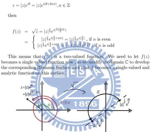
Suppose w; z 2 C and wk = z , we …nd the solution of wk = z in polar form

) wk = z =_{jzj e}i =_jzjei( +2n ) ) w = jzjk1e

i( +2n ) k

where _{2 [} ; ) _{and n 2 Z.}

We will take f (z) =pz = (z)12 for example …rst , where f (z) : C ! C.

We will still use polar form , let

z =_jzjei =_jzjei( +2n ); n_{2 Z} then f (z) = pz =_jzj12ei( +2n 2 ) = ( jzj12ei(2+n ) =jzj 1 2ei(2) , if n is even jzj12ei(2+n ) = ( 1)jzj 1 2ei(2) , if n is odd

This means that f (z) is a two-valued function. We need to let f (z) becomes a single valued function now , so we modify its domain C to develop the corresponding Riemann Surface such that f becomes a single-valued and analytic function on this surface.

Figure 1. The idea of two sheets.

We start at some z = jzjei _{, and then we have f (z) =}p_{z =}p

jzjei(₂)_;

jzj 6= 0_{. Fixing jzj and continuing along a closed path once around the origin so} that increases by 2 , f (z) comes to the value

p

jzjei( +22 ) = pjzjei(2)

which is just the negative of its original value. When we continuing same way above , we …nd that as increases by 2 again , then f (z) comes to oringinal value.

First , we image two sheets lying over the complex plane and cut the plane along negative real axis ( i.e. from 0 to _{1 ) and restrict ourselves such that} never to continue f (z) over this cuts , we get single-valued branches of f (z).

De…ne that f (z) = _jzj12e i 2; < f (z) = _jzj12e i 2; < 3

called sheet-I and sheet-II , respectively. There are two edges for every cut on each sheet , we label the starting edge with (+)-edge and the terminal edge with ( )-edge. (Show in Figure 2)

Figure 2. Complex plane and extended complex plane.

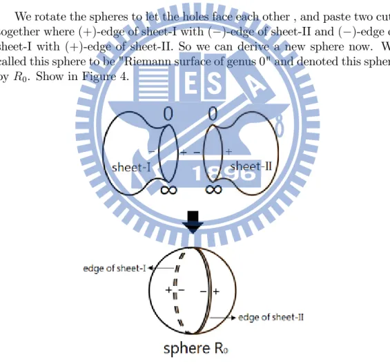
Moreover , when crossing the cut , we pass from one sheet to another. Second , we extend the plane of complex numbers with one additional point at in…nity constitute a number system known as the extended complex numbers. Use stereographic projection , we can consider the two sheets to be a spheres. And we image that the spheres are made of rubber and stretch each cut into circular holes.

Figure 3. Place the cuts open.

We rotate the spheres to let the holes face each other , and paste two cuts together where (+)-edge of sheet-I with ( )-edge of sheet-II and ( )-edge of sheet-I with (+)-edge of sheet-II. So we can derive a new sphere now. We called this sphere to be "Riemann surface of genus 0" and denoted this sphere by R0. Show in Figure 4.

Figure 4. Construct R0.

Notice that in Riemann Surface (+)-edge of sheet-I is equivalent to ( )-edge of sheet-II and ( )-edge of sheet-I is equivalent to (+)-edge of sheet-II.

We could using similar way to develop the corresponding Riemann Surface for f (z) = r n k=1(z zk)

We use two examples to show this , one have odd roots , and the other have even roots.

Example 1 Suppose there are 7 roots where the function f (z) have. Con-struct the Riemann Surface of f (z) =

r 7 k=1(z zk) = 7 k=1 p (z zk); zk 2 R

where z7 < z6 < z5 < z4 < z3 < z2 < z1 and we cut plane starts from zk to

1 , k = 1; 2; 3; 4; 5; 6; 7.

Figure 5. Cut plane start from zk to 1.

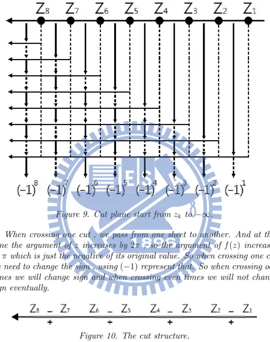
When crossing one cut , we pass from one sheet to another. And at this time the argument of z increases by 2 , so the argument of f (z) increases by which is just the negative of its original value. So when crossing one cut we need to change the sign , using ( 1) represent that. So when crossing odd times we will change sign and when crossing even times we will not change sign eventually.

Figure 6. The cut structure.

There are branch cuts in ( 1; z7] , [z6; z5] , [z4; z3] , [z2; z1] and then

using same idea to construct the corresponding Riemann Surface.

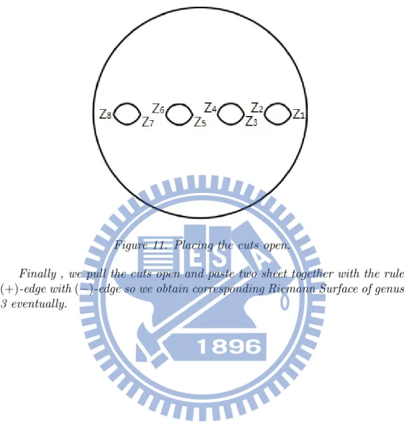
Figure 7. Placing the cuts open.

Finally , we pull the cuts open and paste two sheet together with the rule (+)-edge with ( )-edge so we obtain corresponding Riemann Surface of genus 3 eventually.

Figure 8. Geometric graph of R3.

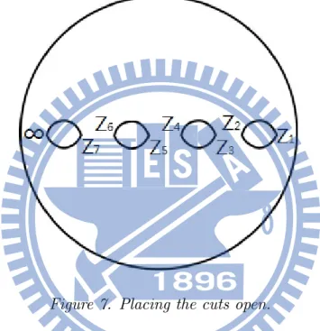
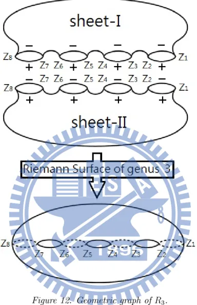
Example 2 Suppose there are 8 roots where the function f (z) have. Con-struct the Riemann Surface of f (z) =

r 8 k=1(z zk) = 8 k=1 p (z zk); zk 2 R

where z8 < z7 < z6 < z5 < z4 < z3 < z2 < z1 and we cut plane starts from zk

Figure 9. Cut plane start from zk to 1.

When crossing one cut , we pass from one sheet to another. And at this time the argument of z increases by 2 , so the argument of f (z) increases by which is just the negative of its original value. So when crossing one cut we need to change the sign , using ( 1) represent that. So when crossing odd times we will change sign and when crossing even times we will not change sign eventually.

Figure 10. The cut structure.

There are branch cuts in [z8; z7] , [z6; z5] , [z4; z3] , [z2; z1] and then using

Figure 11. Placing the cuts open.

Finally , we pull the cuts open and paste two sheet together with the rule (+)-edge with ( )-edge so we obtain corresponding Riemann Surface of genus 3 eventually.

Figure 12. Geometric graph of R3.

Although there are di¤erent algebraic structures between 7 roots and 8 roots that f (z) have. But they both have the same geometric graph with 3 holes. This means that no matter 7 or 8 roots , we can construct correspond-ing Riemann Surface of genus 3.

1.2

The relationship of curve between algebraic

struc-ture and geometric strucstruc-ture.

We will use algebraic to compute the integrals and discuss the integrals later for convenience. We already know the relation of algebraic and geometric structure with f (z) =

r _n

We give some examples to show that the curve in algebraic structure and its corresponding in geometric structure.

We de…ned something as following:

1. The curve in sheet-I is solid line and the curve in sheet-II is dash line in algebraic structure.

2. The curve in overhead Riemann Surface is solid line and the curve in ventral Riemann Surface is dash line in geometric structure.

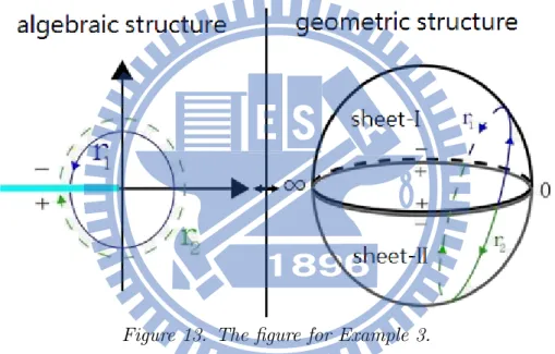
Example 3 r1 is the curve from a point at (I; +) to (I; ) in sheet-I and r2

is the curve from a point at (II; ) to (II; +) in sheet-II.

Figure 13. The …gure for Example 3.

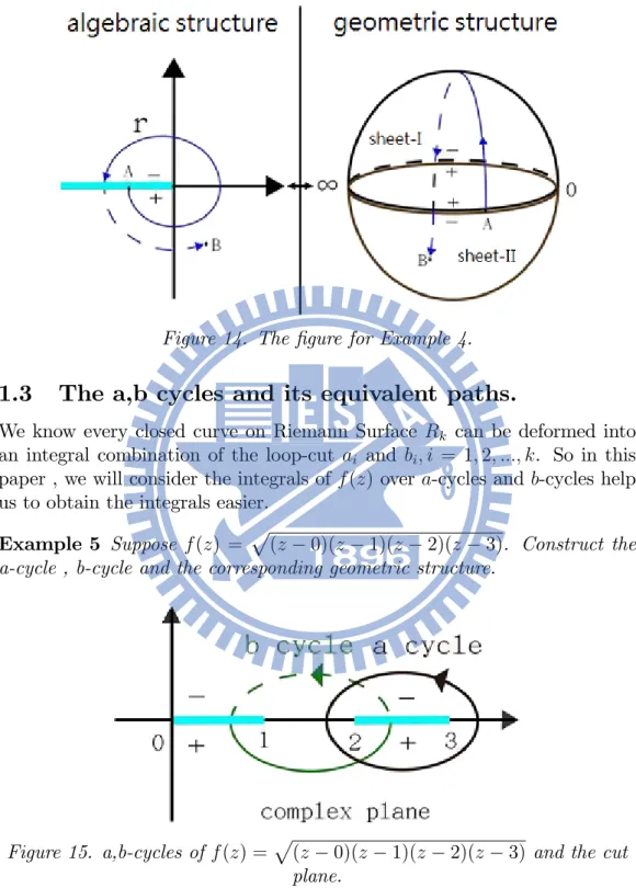
Example 4 The curve r is start from point A in sheet-I and cross the cut to point B on sheet-II.

Figure 14. The …gure for Example 4.

1.3

The a,b cycles and its equivalent paths.

We know every closed curve on Riemann Surface Rk can be deformed into

an integral combination of the loop-cut ai and bi; i = 1; 2; :::; k. So in this

paper , we will consider the integrals of f (z) over a-cycles and b-cycles help us to obtain the integrals easier.

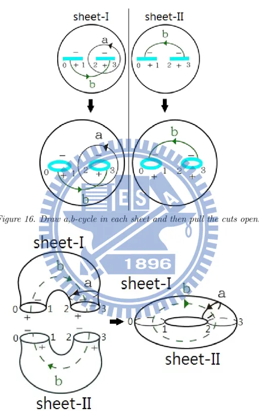
Example 5 Suppose f (z) = p(z 0)(z 1)(z 2)(z 3). Construct the a-cycle , b-cycle and the corresponding geometric structure.

Figure 15. a,b-cycles of f (z) =p(z 0)(z 1)(z 2)(z 3) and the cut plane.

Because f (z) has four roots , so we can construct two cuts and one a-cycle and one b-a-cycle. Notice that in this example , the numbers of a-a-cycle and the numbers of b-cycle are the same.

Figure 16. Draw a,b-cycle in each sheet and then pull the cuts open.

Figure 17. Corresponding geometric structure and cycles.

Finally , we paste two sheets with open cuts and gained corresponding geometric structure and cycles.

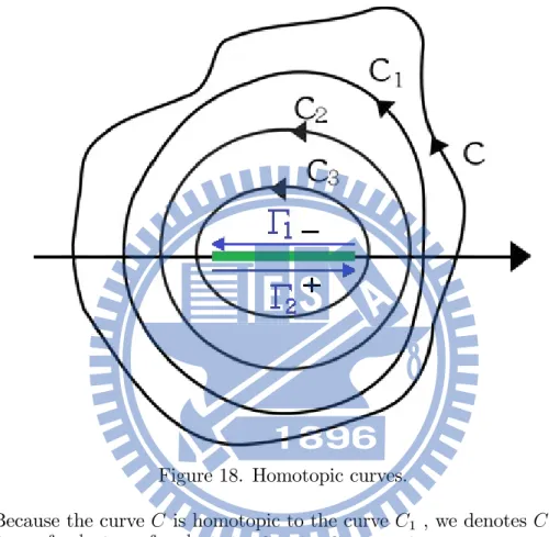
It is di¢ cult to write out the parameters of curves sometimes. But the straight lines are easy to write out their parameters for us. So using homo-topic of curves to …nd the equivalent paths of curves could help us to obtain the integrals over the curves easier and quicker.

Figure 18. Homotopic curves.

Because the curve C is homotopic to the curve C1 , we denotes C t C1.

We have R_C 1 f (z)dz =

R

C1

1

f (z)dz by Cauchy-Goursat theorem. In Figure 18 ,

we see that C t C1 t C2 t C3 t 1[ 2.

Z C 1 f (z)dz = Z C1 1 f (z)dz = Z C2 1 f (z)dz = Z C3 1 f (z)dz = Z 1[ 2 1 f (z)dz = Z 1 1 f (z)dz + Z 1 1 f (z)dz We will use this method in the whole paper.

1.4

Conclusion of Riemann Surface.

Although the result and statement we discuss with above are all in horizontal cut. But the method which handleing other styles of cut is the same as in horizontal cut. We take !2 _{= c(z z}

1)(z z2)(z z3) for an example ,

where z1; z2; z3 2 C are distinct and c is a constant. Because pc does not

in‡uence the cut , so we omitpcand let f (z) =p(z z1)(z z2)(z z3) =

p

(z z1)

p

(z z2)

p

(z z3). Remembering when arg(z zk) changes by

2 , the factorp(z zk) will change the sign. In the …gure 19 we label left

of cut with (+)-edge and right of cut with ( )-edge.

Figure 19. The cut-plane and a; b cycles in each sheets.

We construct the Riemann Surface in similar way before. Imageing both two sheets are made of rubber , and pull cuts to be holes. We rotate the

sheets to let the holes face each other , and paste two cuts together where (+)-edge of sheet-I with ( )-edge of sheet-II and ( )-edge of sheet-I with (+)-edge of sheet-II. We will get the corresponding Riemann Surface R1.

The a; b curves are corresponding to the meridian curve a and latitude curve b on Rienann Surface R1 , respectively.

Figure 20. Corresponding Riemann Surface.

2

The integrations of 1=f (z) over a; b cycles

for cuts on Riemann Surface.

When we known the geometric structure of Riemann Surface. It is usefull to know the integration of a function on Riemann Surface. Especially , the a; b cycles for cuts on Riemann Surface.

2.1

The integrations of

1=f (z) over a; b cycles of the

Riemann Surface with horizontal cut-structure.

We will use Mathematica help us to obtain the values of integrations of 1=f (z) over a; b cycles. First, We discuss the values in sheet-I, sheet-II and Mathematica for horizontal cuts.

In using polar form

1 f (z) = [ n k=1(z zk)] 1 2 = (rei ) 1 2

Let 1 denotes in sheet-I and 2 denotes in sheet-II. Clearly that 2 = 1+ 2 , so we have ( 1 f (z))j(II) = r 1 2ei( 22) = r 12ei( 1+2 2 ) = r 12ei( 21)ei( ) = ( 1)r 12ei( 21) = ( 1)( 1 f (z))j(I)

where (_{f (z)}1 )_j(I) denote the value of _{f (z)}1 with z in sheet-I and (_{f (z)}1 )j(II)

denote the value of _{f (z)}1 with z in sheet-II. Because the di¤erence of argument between z in sheet-I and in sheet-II is 2 , so the di¤erence between (_{f (z)}1 )_j(I)

and ( 1 f (z))j(II) is ( ). Hence , ( 1 f (z))j(II)= ( 1)( 1 f (z))j(I)

Now we discuss the di¤erence over sheet-I in theory and in Mathematica. First , we considerp 1. See Figure 21 , in theory we know thatp 1 = i by the de…nition of argument in sheet-I. But in Mathematica , when we compute p 1 , we will obtain p 1 M ath= i. Actually , we found that rei

where _{2 (} ; ]in Mathematica. This means for any other of rei _which

does not belong to ( ; ] , Mathematica will converse rei into rei where 2 ( ; ] and rei _{= re}i _.

Figure 21. Domain and range of square function in Theory and in Mathematica.

Compare the value of (1=f (z)) with z in sheet-I and in Mathematica , we discover that Lemma 6 If (1=f (z)) = [ n k=1(z zk)] 1 2 = (rei ) 1

2 in sheet-I for horizontal

cut , then ( 1 f (z))j(I) = ( (_{f (z)}1 )_jM athematica , if 2 ( ; ) ( 1)(_{f (z)}1 )_jM athematica , if =

Proof. Since ( ) does not in ( ; ] , then Mathematica will converse rei( ) _{into re}i _{and re}i( ) _{= re}i _{. We compute (1=f (z)) in theory and in}

Mathematica. In theory : r = rei( ) 1 p ! (rei( )₎ 1_{2 = ir} 1₂ In Mathematica : r = rei( ) M ath:_{= re}i 1 p

! (rei ₎ 1₂ M ath:_{= ( 1)ir} 1₂

Hence , (1=f (z))j(I) M ath:

In this whole paper , (1=f (z)) M ath:= ( 1)(1=f (z)) denotes the function (1=f (z)) in front ofM ath:= is the value of (1=f (z)) in theory and the function (1=f (z)) behind theM ath:= is the value of (1=f (z)) in Mathematica. After we known the state above, we must modify the computation when we want to use Mathematica to calculate the value. Take examples to explain.

Example 7 Evaluate R_r 1

f (z)dz where f (z) =

p

(z 1)(z 2)(z 3); z _{2 R} and r = r1 [ r2 where r1 is the path on a horizontal cut from 2 to 3 with

(+)-edge of sheet-I and r2 is the path on a horizontal cut from 3 to 2 with

( )-edge of sheet-I.

Figure 22. Cuts in complex plane of f (z) =p(z 1)(z 2)(z 3) . Solution 8 Since f (z) = p(z 1)(z 2)(z 3) =pz 1pz 2pz 3 1. If z 2 r1 : (1) In theory : z 1 0_{) p} 1 z 1 =jz 1j 1 2 z 2 0_{) p} 1 z 2 =jz 2j 1 2 z 3 < 0_{) z} 3 =_jz 3_je i _{) p} 1 z 3 =jz 3j 1 2ei2 = ijz 3j 1 2 we have Z r1 1 f (z)dz = i Z 3 2 jz 1_j 12jz 2j 1 2jz 3j 1 2dz

(2) In Mathematica : z 1 0_{) p} 1 z 1 =jz 1j 1 2 z 2 0_{) p} 1 z 2 =jz 2j 1 2 z 3 < 0_{) z} 3 =_jz 3_jei _{) p} 1 z 3 =jz 3j 1 2e i2 = ijz 3j 1 2 we have Z r1 1 f (z)dz = i Z 3 2 jz 1_j 12jz 2j 1 2jz 3j 1 2dz

Compare (1) and (2) , we found there is a di¤erence of minus sign with the value in sheet-I and in Mathematica.

2. If z 2 r2 : (1) In theory : z 1 0_{) p} 1 z 1 =jz 1j 1 2 z 2 0_{) p} 1 z 2 =jz 2j 1 2 z 3 < 0_{) z} 3 =_jz 3_jei _{) p} 1 z 3 =jz 3j 1 2e i2 = ijz 3j 1 2 we have Z r2 1 f (z)dz = i Z 2 3 jz 1_j 12jz 2j 1 2jz 3j 1 2dz (2) In Mathematica : z 1 0_{) p} 1 z 1 =jz 1j 1 2 z 2 0_{) p} 1 z 2 =jz 2j 1 2 z 3 < 0_{) z} 3 =_jz 3_jei _{) p} 1 z 3 =jz 3j 1 2e i2 = ijz 3j 1 2

we have Z r2 1 f (z)dz = i Z 2 3 jz 1_j 12jz 2j 1 2jz 3j 1 2dz

Compare (1) and (2) , the value is the same. By 1; 2 we have R r 1 f (z)dz = 2iR₂3_jz 1_j 12 _{jz 2j} 1 2 _{jz 3j} 1 2 _{dz in sheet-I .} 0 in Mathematica . = 0: + 5:24412i in sheet-I . 0 in Mathematica .

Clearly, there is a mistake when = . When we use Mathematica to get the value of integration we want , we need modify some range where the value will wrong. Determine the di¤erence of sign(f ) (same or negative) and then modify the computation of Mathematica to get right value. Because sometimes the form of integration is complex , if we could simplify the way about modify the di¤erence of sign(f ) , it will help us to get right value easier.

Example 9 Same f (z) as the example before , using Lemma in this section to modify. Solution 10 . 1. If z 2 r1; z : 2! 3 z 1 0_{) arg(z} 1) = 0_{) p} 1 z 1 M ath: = _p 1 z 1 z 2 0_{) arg(z} 2) = 0_{) p} 1 z 2 M ath: = _p 1 z 2 z 3 < 0_{) arg(z} 3) = _{) p} 1 z 3 M ath: = _p 1 z 3 we have Z r1 1 f (z)dz M ath: = Z 3 2 1 p z 1 1 p z 2 1 p z 3dz

2. If z 2 r2; z : 3! 2 z 1 0_{) arg(z} 1) = 0_{) p} 1 z 1 M ath: = _p 1 z 1 z 2 0_{) arg(z} 2) = 0_{) p} 1 z 2 M ath: = _p 1 z 2 z 3 < 0_{) arg(z} 3) = _{) p} 1 z 3 M ath: = _p 1 z 3 we have Z r2 1 f (z)dz M ath: = Z 2 3 1 p z 1 1 p z 2 1 p z 3dz By 1; 2 we have Z r 1 f (z)dz M ath: = 2 Z 3 2 1 p z 1 1 p z 2 1 p z 3dz = 0: + 5:24412i

Example 11 Evaluate R _{f (z)}1 dz over a1 , a2 and a3 cycles where f (z) =

p

(z + 4)(z + 2)(z 2)(z 4)(z 5)(z 7)(z 8). We analysis the integral in Mathematica and in theory to compare the result and using the result of angle to modify the computation to get value. Let z1 = 8 , z2 = 7 , z3 = 5 ,

z4 = 4 , z5 = 2 , z6 = 2 , z7 = 4.

Figure 23. a-cycles and their equivalent path a .

Solution 12 The detail is in appendix. And we just only give numerical solution here.

Z a1 1 f (z)dz M ath: = 0: + 0:0890282i Z a2 1 f (z)dz M ath: = 0: + 0:1832730i Z a3 1 f (z)dz M ath: = 0: + 0:1115720i

Example 13 Evaluate R _{f (z)}1 dz over b1 , b2 and b3 cycles where f (z) =

p

(z + 4)(z + 2)(z 2)(z 4)(z 5)(z 7)(z 8). We analysis the inte-gral in Mathematica and in theory to compare the result and using the result of angle to modify the computation to get value. Let z1 = 8 , z2 = 7 , z3 = 5

, z4 = 4 , z5 = 2 , z6 = 2 , z7 = 4.

Figure 24. b1 , b2 and b3 cycles.

Solution 14 The detail is in appendix. And we just only give numerical solution here. Z b1 1 f (z)dz M ath: = 0:4132335 Z b2 1 f (z)dz M ath: = 0:2196815 Z b3 1 f (z)dz M ath: = 0:0372385

2.2

The integrations of

1=f (z) over a; b cycles of the

Riemann Surface with vertical cut-structure.

After knowing the integrations in horizontal cut , we will discuss the integra-tions for vertical cuts. In this case , we de…ne that

z zk =

rei _;

2 [ 32 ; 2) i¤ z in sheet-I

rei ; _{2 [2};5₂ ) i¤ z in sheet-II

the cut in each sheet has two edges , label the starting edge with (+)-edge and the terminal edge with ( )-edge and zk is the end point of the vertical

cut.

First , we will analysis the value of 1=f (z) on sheet-I and sheet-II in theory.

Second , we will discuss the di¤erence between the value of 1=f (z) in theory and in Mathematica and …nd out how to modify the computation.

1. Analysis the value of 1=f (z) on sheet-I and sheet-II in theory : For a simple case f (z) =pz , by the …gure below , we know that if z =jzj e

i _where

2 [ 32 ;2) i.e. z = jzj e i

2 sheet-I z =_{jzj e}i where _{2 [2};5₂ ) _{i.e. z = jzj e}i _{2 sheet-II} , then ( p z =_jzj12 _ei2; 2 2 [ 3 4 ; 4) p z =_jzj12 ei2; 2 2 [4; 5 4 ) Figure 25. Case of f (z) =pz. and ( 1=pz =_jzj 12 _ei( 2); 2 2 ( 4; 3 4 ] 1=pz =_jzj 12 _ei( 2); 2 2 ( 5 4 ; 4]

Figure 26. Case of f (z) = 1=pz. For the general case , suppose f (z) =

r _n k=1(z zk) , then 8 > < > : n k=1(z zk) = re i 1_; 1 2 [ 3₂ ;₂) in sheet-I n k=1(z zk) = re i 2_; 2 2 [₂;5₂ ) in sheet-II

From the idea of de…nition , rei 1 _{= re}i 2 _and

2 = 1+ 2 , we have ( 1 f (z))j(II) = r 1 2ei( 22) = r 12ei( 1+2 2 ) = r 12ei( 21)ei( ) = ( 1)r 12ei( 21) = ( 1)( 1 f (z))j(I)

2. Discuss the di¤erence between the value of 1=f (z) in theory and in Mathematica and …nd out how to modify the computation :

In the Figure below , we see the value of f (z) =pz in sheet-I and the value of f (z) =pz in Mathematica. So we need to modify the compu-tation in Mathematica such that the numerical result of Mathematica is identical to the numerical result of theory when _{2 [} 3₂ ; ].

Figure 27. The value of f (z) =pz in sheet-I and in Mathematica. Lemma 15 When z in sheet-I for vertical cut whose one of the end points is zk , we have 1 p z zk M ath: = ( ( 1)_p 1 z zk if arg(z zk)2 [ 3 2 ; ] , 1 p z zk if arg(z zk)2 ( ;2)

Proof. Let z in sheet-I and using polar form z zk= rei . When 2 ( ;₂)

, the argument in theory or Mathematica is the same. When _{2 [} 3₂ ; ] , Mathematica will conversion _{2 [} 3₂ ; ] into + 2 _{2 [2}; ] and rei ₌

rei( +2 ) = rei +i(2 ) , but ( In theory : (z zk) 1 2 = (rei ) 1 2 = r 1 2ei( 2) In Mathematica : (z zk) 1 2 = (rei +i(2 )) 1 2 = ( 1)r 1 2ei( 2) So if _{2 [} 3₂ ; ] , we have 1 p z zk M ath: = ( 1)_p 1 z zk

As same as horizontal cut , we …rst discuss the di¤erence of values of 1=f (z) between sheet-I and sheet-II in theory. And discuss the value of 1=f (z) in theory and in Mathematica , compare their sign(f ) is di¤erent or not? Using statement before and modify to get the value. The result is similar to horizontal cut.

Example 16 Evaluate the integrals of 1=f (z) over a1 cycle for vertical cut

where f (z) = p(z i)(z 2i)(z 3i)(z 5i)(z 6i)(z 8i).

Figure 28. path a and its equivalent path a .

Solution 17 In the Figure 28. , we know that a₁ is an equivalent path for a1 and a1 is the path along vertical cut from 2i to i on (+)-edge of sheet-I

(called a₁₁) and then back from i to 2i on ( )-edge of sheet-I (called a₁₂). So we compute R_a

1

1 f (z)dz.

1. a₁₁ : Let z = ri where r : 2_{! 1 and dz = idr}+ (1) Analysis in theory :

Since z ki = _jz ki_{j e}i arg(z ki) _{, so we consider arg(z ki).}

arg(z i) = 3 2 ) arg( 1 p z i) = 3 4 arg(z ki) = 1 2 ) arg( 1 p z ki) = 4; k = 2; 3; 5; 6; 8 we have

1 f (z) = ( 8 k=1;k6=4;7jz kij 1 2)(e 3 4 )(e4)5 = ( 8 k=1;k6=4;7jz kij 1 2)(e2 ) = ( 8 k=1;k6=4;7jz kij 1 2₎ = R

(2) Analysis in Mathematica (no matter in which sheet) :

Since z ki = _jz ki_{j e}i arg(z ki) _{, so we consider arg(z ki).}

arg(z i) = 1 2 ) arg( 1 p z i) = 4 arg(z ki) = 1 2 ) arg( 1 p z i) = 4; k = 2; 3; 5; 6; 8 we have 1 f (z) = ( 8 k=1;k6=4;7jz kij 1 2)(e 4)(e4)5 = ( 8 k=1;k6=4;7jz kij 1 2)(e ) = ( 8 k=1;k6=4;7jz kij 1 2_{)( 1)} = R

Compare with (1) and (2) we …nd that when we want to obtain true value, the value which we have from Mathematica should multiply ( 1) , i.e. sign(f (z)j(I)) = ( 1)sign(f (z)jM athematica).

(3) Using the Lemma 15 to modify :

arg(z i) = 3 2 ) 1 p z i M ath: = ( 1)_p 1 z i arg(z ki) = 1 2 ) 1 p z i M ath: = _p 1 z ki; k = 2; 3; 5; 6; 8 we have

1 f (z)

M ath:

= ( 1) 1 f (z)

The same result as above di¤erence between in theory and in Math-ematica , the di¤erence is a minus sign.

2. a_{12 : Let z = ri where r : 1 ! 2 and dz = idr} (1) Analysis in theory :

Since z ki = _jz ki_{j e}i arg(z ki) , so we consider arg(z ki).

arg(z i) = 1 2 ) arg( 1 p z i) = 4 arg(z ki) = 1 2 ) arg( 1 p z ki) = 4; k = 2; 3; 5; 6; 8 we have 1 f (z) = ( 8 k=1;k6=4;7jz kij 1 2_)(e 4)(e4)5 = ( 8 k=1;k6=4;7jz kij 1 2)(e ) = ( 8 k=1;k6=4;7jz kij 1 2_{)( 1)} = R

(2) Analysis in Mathematica (no matter in which sheet) :

Since z ki = _jz ki_{j e}i arg(z ki) _{, so we consider arg(z ki).}

arg(z i) = 1 2 ) arg( 1 p z i) = 4 arg(z ki) = 1 2 ) arg( 1 p z ki) = 4; k = 2; 3; 5; 6; 8 we have

1 f (z) = ( 8 k=1;k6=4;7jz kij 1 2_)(e 4)(e4)5 = ( 8 k=1;k6=4;7jz kij 1 2_{)(e )} = ( 8 k=1;k6=4;7jz kij 1 2)( 1) = R

Compare with (1) and (2) we …nd the value is same.

(3) Using the Lemma 15 to modify :

arg(z i) = 1 2 ) 1 p z i M ath: = _p 1 z i arg(z ki) = 1 2 ) 1 p z i M ath: = _p 1 z ki; k = 2; 3; 5; 6; 8 we have 1 f (z) M ath: = 1 f (z)

The same result as above.

By 1: and 2: above , we have

Z a1 1 f (z)dz = Z a₁ 1 f (z)dz = Z a₁₁ 1 f (z)dz + Z a₁₂ 1 f (z)dz = 2 Z 1 2 ( 8 k=1;k6=4;7jri kij 1 2)idr = 0: 0:531987i

Example 18 Evaluate the integrals of 1=f (z) over a; b cycles for vertical cut where f (z) = p(z i)(z 2i)(z 3i)(z 5i)(z 6i)(z 8i).

We can integrate 1=f (z) over a; b cycles of the Riemann Surface with horizontal cut-structure and with vertical cut-structure. We give some more examples here , and the solution could see in appendix.

Example 20 Compute the integrals of 1=f (z) over every cycles in the Figure below where

f (z) =p(z z1)(z z2)(z z3)(z z4)(z z5)(z z6)(z z7)(z z8)

for z1 = 2 i; z2 = 2 + i; z3 = 1 i; z4 = 1 + i; z5 = 0 + 0i; z6 =

0 + i; z7 = 1 + i; z8 = 1 + 2i.

Figure 29. cycles a1; a2; a3 and equivalent pathes a1; a2; a3.

Figure 31. Cycle b3 and equivalent path b3.

2.3

The integrations of the Sine-Gordon Equation over

a; b cycles.

Now we want to compute the integral

Z ₁

q

( 1)u₁2 + u₁₂4 ₃₆₀u6 +₂₀₁₆₀u8 _1814400u10 +_239500800u12 + 2k du

over a; b cycles.

Let k = 1 , and compute the roots of the equation

( 1)u 2 1 + u4 12 u6 360 + u8 20160 u10 1814400 + u12 239500800 + 2k = 0 We have the roots of the equation

( 1)u 2 1 + u4 12 u6 360 + u8 20160 u10 1814400 + u12 239500800 + 2 = 0

are similar to Z1 = 6:58948 + 5:23118i , Z2 = 6:58948 5:23118i ,

Z3 = 6:31381 + 1:46139i, Z4 = 6:31381 1:46139i, Z5 = 4:68652 + 0:0i

, Z6 = 1:57080 + 0:0i , Z7 = 1:57080 + 0:0i , Z8 = 4:68652 + 0:0i , Z9 =

6:31381 + 1:46139i , Z10 = 6:31381 1:46139i , Z11 = 6:58948 + 5:23118i ,

Z12 = 6:58948 5:23118i.

Figure 32. Zi; i2 f1; 2; 3; 4; 5; 6; 7; 8; 9; 10; 11; 12g and its cuts.

First , we will compute the integral of 1=f (z) over a1; a2; a3; a4; a5 cycles

in the Figure 33 below where

f (z) =

12 k=1

p

(z zk)

and Z1 = 6:58948 + 5:23118i , Z2 = 6:58948 5:23118i , Z3 =

6:31381 + 1:46139i , Z4 = 6:31381 1:46139i , Z5 = 4:68652 + 0:0i

, Z6 = 1:57080 + 0:0i , Z7 = 1:57080 + 0:0i , Z8 = 4:68652 + 0:0i ,

Z9 = 6:31381+1:46139i, Z10= 6:31381 1:46139i, Z11 = 6:58948+5:23118i

Figure 33. a1; a2; a3; a4; a5 cycles and its equivalent path a1; a2; a3; a4; a5.

Z a1 1 f (z)dz = 9:52646 10 18_{+ 0:000197837i} Z a2 1 f (z)dz = 2:31913 10 14 _0:000472233i Z a3 1 f (z)dz = 2:23575 10 14_{+ 0:000472233i} Z a4 1 f (z)dz = 9:52151 10 18 0:000197837i Z a5 1 f (z)dz = 1:54107 10 17_{+ 0:000262034i}

Second , we will compute the integral of 1=f (z) over b1; b2; b3; b4; b5 cycles

in the Figure 34 below where

f (z) =

12 k=1

p

(z zk)

and Z1 = 6:58948 + 5:23118i , Z2 = 6:58948 5:23118i , Z3 =

6:31381 + 1:46139i , Z4 = 6:31381 1:46139i , Z5 = 4:68652 + 0:0i

, Z6 = 1:57080 + 0:0i , Z7 = 1:57080 + 0:0i , Z8 = 4:68652 + 0:0i ,

Z9 = 6:31381+1:46139i, Z10= 6:31381 1:46139i, Z11 = 6:58948+5:23118i

, Z12 = 6:58948 5:23118i.

Similarly , we will just write solution here , and the calculation is putted in appendix. Z b1 1 f (z)dz = 0:0000106043 0:0000764721i Z b2 1 f (z)dz = 0:00025277 + 0:0000169501i Z b3 1 f (z)dz = 0:000226449 + 0:0000169501i Z b4 1 f (z)dz = 0:0000523241 + 0:000115868i Z b5 1 f (z)dz =

The integrations of the equation over a; b cycles above are all numerical approximation. Can we get exact solution of the Sine-Gordon equation? We need more tools in Mathematics.

3

The Elliptic functions , the Theta functions

, and the Jacobian Elliptic functions.

When we handle the problem before. It is useful for us to know about the Elliptic functions , the Theta functions and the Jacobian Elliptic functions.

3.1

The Elliptic Functions.

De…nition 21 A function f (z) is called a doubly-periodic function of z with periods 2!1 , 2!2 , if function f (z) satis…es the equations below for all values

of z for which f (z) exists.

f (z + 2!1) = f (z)

f (z + 2!2) = f (z)

Where !1 , !2 are any two numbers (complex or real) whose ratio is not

purely real.

De…nition 22 A doubly-periodic function which is analytic (except at poles) , and which has no singularities other than poles in the …nite part of the plane , is called an elliptic function.

In mathematics , a singularity is in general a point at which a given mathematical object is not de…ned , or a point of an exceptional set where it fails to be well-behaved in some particular way , such as di¤erentiability.

Remark 23 Suppose f is a complex di¤erentiable function de…ned on some neighborhood Np around point p , excluding point p i.e. Np fpg , where Np

is an open subset of the complex numbers C , and the point p is an element of Np. There are four classes of singularities in complex analysis.

1. Isolated singularities : Suppose the function f is not de…ned at p , although it does have values de…ned on Np fpg.

(1) The point p is a removable singularity of f if there exists a holo-morphic function g de…ned on all of Np such that f (z) = g(z) for

all z in Np fpg. The function g is a continuous replacement for

the function f .

(2) The point p is a pole or non-essential singularity of f if there exists a holomorphic function g de…ned on Np and a natural number n

such that f (z) = _{(z p)}g(z)n for all z in Np fpg. The derivative at a

non-essential singularity may or may not exist. If g(p) is nonzero , then we say that p is a pole of order n.

(3) The point p is an essential singularity of f if is neither a removable singularity nor a pole. The point p is an essential singularity if and only if the Laurent series has in…nitely many powers of negative degree.

2. Branch points are generally the result of a multi-valued function, such as pz or log(z) being de…ned within a certain limited domain so that the function can be made single-valued within the domain. The cut is a line or curve excluded from the domain to introduce a technical separation between discontinuous values of the function. When the cut is genuinely required , the function will have distinctly di¤erent values on each side of the branch cut. The location and shape of most of the branch cut is usually a matter of choice , with perhaps only one point (like z = 0 for log(z)) which is …xed in place.

De…nition 24 A period-parallelogram is called a cell if there are none of the poles of the integrands considered on the sides of the parallelogram.

De…nition 25 A set is called an irreducible set if it is a set of poles ( or zeros ) of an elliptic function in any given cell.

Remember that all other poles ( or zeros ) of the elliptic function outside the irreducible set are congruent to one or other of them.

There are some simple properties of elliptic functions.

1. The number of poles of an elliptic function in any cell is …nite.

Proof. Suppose that the number of poles of an elliptic function f (z) in some cell is not …nite , then the poles must have a limit point p. Clearly , this point p is a singularity but not a pole. So by de…nition of elliptic function , the function f (z) is not an elliptic function. (! ) 2. The number of zeros of an elliptic function in any cell is …nite.

Proof. Suppose the number of zeros of an elliptic function f (z) in some cell is not …nite , then 1=f (z) is an elliptic function which have in…nite poles in this cell. But this is a contradiction by elliptic function simple property 1.

3. The sum of the residues of an elliptic function , f (z) , at its poles in any cell is zero.

Proof. Suppose the corners of the cell are t; t+2!1; t+2!1+2!2; t+2!2.

Let C be the contour formed by the edges of the cell. The sum of the residues of f (z) at its poles inside C is

1 2 i Z C f (z)dz = 1 2 i Z t+2!1 t + Z t+2!1+2!2 t+2!1 + Z t+2!2 t+2!1+2!2 + Z t t+2!2 f (z)dz

Let x = z 2!1 , then dz = dx , thus

1 2 i Z t+2!1+2!2 t+2!1 f (z)dz = 1 2 i Z t+2!2 t f (x + 2!1)dx = 1 2 i Z t+2!2 t f (z + 2!1)dz = 1 2 i Z t+2!2 t f (z)dz

1 2 i Z t+2!2 t+2!1+2!2 f (z)dz = 1 2 i Z t t+2!1 f (y + 2!2)dy = 1 2 i Z t t+2!1 f (z + 2!2)dz = 1 2 i Z t t+2!1 f (z)dz So we have 1 2 i Z C f (z)dz = 1 2 i Z t+2!1 t + Z t+2!2 t + Z t t+2!1 + Z t t+2!2 f (z)dz = 0

4. (Liouville’s Theorem) An elliptic function , f (z) , with no poles in a cell is merely a constant.

Proof. Suppose f (z) has no poles inside the cell. * f(z) is analytic inside and on the boundary of the cell. ) f(z) is bounded inside and on the boundary of the cell. )there exists a number K 2 R such that jf(z)j < K when z is inside or on the boundary of the cell. * f(z) is a doubly-periodic function and f (z) is analytic and jf(z)j < K for all values of z. ) f(z) is a constant.

Let f (z) be an elliptic function and C be any cell with corners t; t + 2!1; t + 2!1 + 2!2; t + 2!2 and a be any constant. Because the di¤erence

between the number of zeros of f (z) a and the number of poles of f (z) a which lie in the cell C is

1 2 i Z C f0_(z) f (z) adz

When we try to compute its value. Since f (z) is an elliptic function , thus f0(z + 2!1) = f0(z + 2!2) = f0(z).

1 2 i Z t+2!1+2!2 t+2!1 f0_(z) f (z) adz = 1 2 i Z t+2!2 t f0_{(x + 2!} 1) f (x + 2!1) a dx = 1 2 i Z t+2!2 t f0(z + 2!1) f (z + 2!1) a dz = 1 2 i Z t+2!2 t f0(z) f (z) adz Let y = z 2!2 , then dz = dy , so we have

1 2 i Z t+2!2 t+2!1+2!2 f0_(z) f (z) adz = 1 2 i Z t t+2!1 f0_{(y + 2!} 2) f (y + 2!2) a dy = 1 2 i Z t t+2!1 f0_{(z + 2!} 2) f (z + 2!2) a dz = 1 2 i Z t t+2!1 f0_(z) f (z) adz Hence , we have 1 2 i Z C f0_(z) f (z) adz = 0

Therefore the number of zeros of f (z) ais equal to the number of poles of f (z) a. Because any pole of f (z) a is also a pole of f (z) and conversely. Hence the number of zeros of f (z) ais equal to the number of poles of f (z) , which is independent of a. So we have the following de…nition.

De…nition 26 The order of an elliptic function f (z) is the number n of roots of the equation

f (z) = a

which lie in any cell depends only on f (z) , but not on a. And this number n is also equal to the number of poles of f (z) in the cell.

Remark 27 The order of an elliptic function is never less than 2.

Proof. Suppose an elliptic function f (z) of order 1 would have a single irreducible pole ; and if this point actually were a pole ( and not an ordinary point ) the residue there would not be zero , which is contrary to the simple property 3 of elliptic functions.

Remark 28 The simplest elliptic functions are those of order 2. There are two classes of such functions :

1. Function have a single irreducible double pole with residue is 0.

2. Function have two simple poles with the residues are numerically equal but opposite in sign.

Lemma 29 The sum of the a¢ xes of the zeros minus the sum of the a¢ xes of the poles is a period.

Proof. With the notation previously employed. Because the di¤erence be-tween the sums of the zeros and the sums of the poles is

1 2 i Z C zf0_(z) f (z) dz = 1 2 i Z t+2!1 t zf0_(z) f (z) (z + 2!2)f0(z + 2!2) f (z + 2!2) dz 1 2 i Z t+2!2 t zf0_(z) f (z) (z + 2!1)f0(z + 2!1) f (z + 2!1) dz = 1 2 i 2!2 Z t+2!1 t f0(z) f (z)dz + 2!1 Z t+2!2 t f0(z) f (z)dz = 1 2 i 2!2 log f (z)j t+2!1 t + 2!1 log f (z)jt+2!t 2 = 1 2 i 2!2 log f (t + 2!1) f (t) + 2!1 log f (t + 2!2) f (t) = 1 2 i 2!2 log f (t) f (t) + 2!1 log f (t) f (t) = 1 2 if 2!2[log(1)] + 2!1[log(1)]g

on making use of the substitutions used in simple property 3 of elliptic functions and of the periodic properties of f (z) and f0_(z).

* e2k i = cos(2k ) + i sin(2k ) = 1 ) log(1) = log(e2k i) = 2k i

for all k 2 Z. Thus , 1 2 i Z C zf0(z) f (z) dz = 1 2 if 2!2[log(1)] + 2!1[log(1)]g = 1 2 if 2!2( 2n i) + 2!1(2m i)g = 2m!1+ 2n!2 where m; n 2 Z.

3.2

Weierstrass Elliptic function.

After knowing some basic properties of elliptic function. We will introduce the Weierstrass elliptic function.

De…nition 30 The Weierstrass elliptic function }(z) is de…ned by the equa-tion }(z) = 1 z2 + X m;n 0 1 (z 2m!1 2n!2)2 1 (2m!1+ 2n!2)2

The summation extends over all integer values ( positive , negative , and zero ) of m and n , but simultaneous zero values of m and n excepted.

Throughout this paper we will use the notation P

m;n

to denote a summation over all integer values of m and n , and using P

m;n

0 _{when the term for which}

m = n = 0 has to be omitted from the summation. Sometimes , for brevity , we write m;n in place of 2m!1+ 2n!2 , so that

}(z) = 1 z2 + X m;n 0 1 (z 2m!1 2n!2)2 1 (2m!1+ 2n!2)2 = z 2+X m;n 0 (z m;n) 2 m;n2

Remark 31 _{When m; n such that j} m;nj is large , the general terms of the

series de…ning }(z) is O(j m;nj 3). Hence }(z) converges absolutely and

Remark 32 }(z) is analytic except the poles , namely the points m;n and

the points m;n are all double poles.

We now proceed to discuss properties of }(z) and properties of }0_(z).

1. Periodicity and other properties of }(z).

Since }(z) is a uniformly convergent series of analytic functions , term-by-term di¤erentiation is legitimate , hence

}0(z) = d dz}(z) = 21 z3 + X m;n 0 2 1 (z m;n)3 = 2X m;n 1 (z m;n)3

Since the set of points m;n is the same as the set m;n , and the

series for }0_{(z) being absolutely convergent. The derangement of the}

terms does not a¤ect its sum , thus

}0( z) = 2X m;n 1 ( z m;n)3 = " 2X m;n 1 (z + m;n)3 # = " 2X m;n 1 (z m;n)3 # = }0(z)

Hence the function }0_{(z)is an odd function of z.}

In similar manner , the series for }(z) being absolutely convergent. The derangement of the terms does not a¤ect its sum , thus

}( z) = 1 ( z)2 + X m;n 0 1 ( z m;n)2 1 ( m;n)2 = 1 (z)2 + X m;n 0 1 (z + m;n)2 1 ( m;n)2 = 1 (z)2 + X m;n 0 1 (z m;n)2 1 ( m;n)2 = }(z)

Hence the function }(z) is an even function of z.

In similar manner , the series for }0_{(z) being absolutely convergent.}

The derangement of the terms does not a¤ect its sum , thus

}0(z + 2!1) = 2 X m;n 1 (z m;n+ 2!1)3 = 2X m;n 1 (z 2m!1 2n!2 + 2!1)3 = 2X m;n 1 (z 2(m 1)!1 2n!2)3 = 2X m;n 1 (z m 1;n)3 = 2X m;n 1 (z m;n)3 = }0(z)

Hence the function }0_{(z) has the period 2!}

1 , in similar manner the

function }0_{(z) has the period 2!} 2.

Since }0(z)is analytic except at its poles , and }0(z)is a doubly-periodic function. Hence }0_{(z) is an elliptic function.}

If we integrate the equation }0_{(z + 2!}

1) = }0(z) , we get

where K is a constant. Putting z = !1 into the equation }(z +2!1) =

}(z) + K , we have

}( !1+ 2!1) = }( !1) + K

Since }(z) is an even function , we have

}(!1) = }( !1) + K

= }(!1) + K

) K = 0 , this shows that }(z + 2!1) = }(z). In similar manner

}(z + 2!2) = }(z). Since }(z) is a doubly-periodic function , and

}(z) has no singularities but poles , it follows that }(z) is an elliptic function.

We give the following table as conclusion.

Function De…nition Periods Parity Poles }(z) _z12 + P m;n 0n 1 (z m;n)2 1 ( m;n)2 o 2!1; 2!2 even m;n }0_{(z) 2}P m;n 1 (z m;n)3 2!1; 2!2 odd m;n

2. The di¤erential equation satis…ed by }(z). Let f (z) = }(z) z 2 ₌ P

m;n 0 _(z

m;n) 2 m;n2 is analytic in

a region of which the origin is an internal point , and it is an even function of z. By Taylor’s theorem , we have

f (z) = 1 X k=0 f(k)₍₀₎ k! z k = f (0) + f0(0)z +f (2)₍₀₎ 2! z 2₊ f (3)₍₀₎ 3! z 3₊ f (4)₍₀₎ 4! z 4₊ = X m;n 0 2( m;n) 3 z + X m;n 0f6( m;n) 4g 2 z 2 +X m;n 0f 24( m;n) 5g 6 z 3₊X m;n 0f120( m;n) 6g 24 z 4₊ = X m;n 0 2( m;n) 3 z + X m;n 0 3( m;n) 4 z2 +X m;n 0 4( m;n) 5 z3+ X m;n 0 5( m;n) 6 z4+

Since f (z) is an even function of z , )

f (z) = f ( z) = X m;n 0 +2( m;n) 3 z + X m;n 0 3( m;n) 4 z2 +X m;n 0 +4( m;n) 5 z3+ X m;n 0 5( m;n) 6 z4+

2f (z) = f (z) + f ( z) = X m;n 0 2( m;n) 3 z + X m;n 0 3( m;n) 4 z2 +X m;n 0 4( m;n) 5 z3+ X m;n 0 5( m;n) 6 z4 +X m;n 0 +2( m;n) 3 z + X m;n 0 3( m;n) 4 z2 +X m;n 0 +4( m;n) 5 z3+ X m;n 0 5( m;n) 6 z4+ = 2 ( X m;n 0 3( m;n) 4 z2+ X m;n 0 5( m;n) 6 z4+ )

So we have }(z) z 2 = ₂₀1g2z2+₂₈1 g3z4+ O(z6)for su¢ ciently small

values of jzj where g2 = 60 X m;n 0 ( m;n) 4; g3 = 140 X m;n 0 ( m;n) 6 and }(z) = z 2+ 1 20g2z 2₊ 1 28g3z 4_{+ O(z}6₎

di¤erentiating the equation , we have

}0(z) = 2z 3+ 1 10g2z +

1 7g3z

3_{+ O(z}5₎

Cubing }(z) and squaring }0_{(z)respectively , we have}

(}(z))3 = z 6+ 3 20g2z 2 ₊ 3 28g3+ O(z 2₎ (}0(z))2 = 4z 6 2 5g2z 2 4 7g3+ O(z 2₎

Hence

(}0(z))2 4(}(z))3 = g2z 2 g3 + O(z2)

and so

(}0(z))2 4(}(z))3+ g2}(z) + g3 = O(z2)

) the function (}0_(z))2 _4(}(z))3_{+ g}

2}(z) + g3 is analytic at the origin.

Since the function (}0(z))2 4(}(z))3+g2}(z)+g3is an elliptic function ,

so it is also analytic at all congruent points about the origin point. Since such points are the only possible singularities , so the function (}0_(z))2

4(}(z))3+g2}(z)+g3 is an elliptic function with no singularities. Hence

(}0_(z))2 _4(}(z))3 _{+ g}

2}(z) + g3 is a constant by the simple property

4 of elliptic functions. And we can make z ! 0 to gain the di¤erential equation

(}0(z))2 = 4(}(z))3 g2}(z) g3

Hence the function }(z) satis…es the di¤erential equation

(y0)2 = 4y3 g2y g3 where g2 = 60 X m;n 0 ( m;n) 4; g3 = 140 X m;n 0 ( m;n) 6

Conversely , if numbers !1; !2 can be determined such that

g2 = 60 X m;n 0 ( m;n) 4; g3 = 140 X m;n 0 ( m;n) 6

then the general solution of the di¤erential equation (dy_dz)2 = 4y3 g2y

y = }( z + )

where is the constant of integration. Since }(z) is an even function of z , we can write y = }(z + ) without loss of generality.

3. The integral formula for }(z). When we consider the equation

z = Z 1

(4t3 g2t g3)

1 2dt

where the path of integration may be any curve which does not pass through a zero of 4t3 g2t g3.

By The Fundamental Theorem Of Calculus , when we di¤erentiate the equation z = Z 1 (4t3 g2t g3) 1 2dt

we get the equation

(d dz) 2 = 4 3 g2 g3 and so = }(z + )

where is a constant. Since z =R1(4t3 g2t g3)

1

2dt ! 0 as ! 1.

So is a pole of the function }(z) i.e. is of the form m;n , thus

= }(z + ) = }(z + m;n)

So the equation z =R1(4t3 _g

2t g3)

1

2dtis called the integral formula

for }(z) , and it is sometimes written as

z = Z 1 }(z) (4t3 g2t g3) 1 2dt

4. The addition-theorem for the function }(z).

We want to express }(z + y) as an algrbraic function of }(z) and }(y) for general values of z and y. Consider the equations

}0(z) = A}(z) + B; }0(y) = A}(y) + B

which determine A and B in terms of z and y unless }(z) = }(y) , i.e. unless z y(mod :2!1; 2!2). Since

}(z) = 1 z2+ X m;n 0 1 (z m;n)2 1 ( m;n)2 ; }0(z) = 2X m;n 1 (z m;n)3 , so the function }0(x) A}(x) B

has a triple pole at x = 0 and it has three , and only three , irreducible zero.( the number of roots of f (z) is equal to the number of poles of f (z) ).

Since the sum of the zeros minus the sum of the poles is a period. So if x = z; x = y are two zeros , the third irreducible zero must be congruent to z y , i.e. z yis a zero of }0_{(x) A}(x) B. Thus}

}0( z y) = A}( z y) + B Eliminating A and B from the equations

}0(z) = A}(z) + B }0(y) = A}(y) + B }0( z y) = A}( z y) + B we have }(z) }0_{(z) 1} }(y) }0_{(y) 1} }(z + y) }0_{(z + y) 1} = 0

It is called an addition-theorem for the function }(z).

Remark 33 The following equation is another form of the addition-theorem }(z + y) = 1 4 }0_{(z) }}0_(y) }(z) }(y) 2 }(z) }(y)

This equation expresses }(z + y) explicitly in terms of functions of z and y.

5. The duplication formula for }(z).

Taking the limiting form of the equation }(z + y) = 1₄n}_{}(z) }(y)}0(z) }0(y)o

2

}(z) }(y) when y approaches z , we have

lim y!z}(z + y) = 1 4limy!z }0(z) }0(y) }(z) }(y) 2 }(z) lim y!z}(y)

}(2z) = 1 4h!0lim }0(z) }0(z + h) }(z) }(z + h) 2 2}(z) = 1 4h!0lim h}00(z) h}0_(z) 2 2}(z) = 1 4 }00(z) }0_(z) 2 2}(z)

by the de…nition of derivative.

When 2z is not a period , the equation

}(2z) = 1 4 }00(z) }0_(z) 2 2}(z)

is called the duplication formula.

6. The constants e1; e2; e3.

We want to claim that if }(!1) = e1; }(!2) = e2; }(!3) = e3 are all

unequal where !3 = !1 !2 , then e1; e2; e3 are the roots of the

equation

4y3 g2y g3 = 0

(1) Since }0_{(z) is an odd periodic function , we have}

}0(!1) = }0( ( !1)) = }0( !1) = }0( !1+ 2!1) = }0(!1) and so }0(!1) = 0

Similarly ,

}0(!2) = }0(!3) = 0

This means that }0_{(z)has three zeros. Since }}0_{(z) = 2}P m;n

1 (z m;n)3

is an elliptic function whose only singularities are triple poles at points congruent to the origin. Therefore that }0(z) has three , and only three irreducible zeros which are points congruent to !1; !2; !3.

(2) Since }0_{(z) has three irreducible zeros , thus }(z) has only two}

irreducible poles. Clearly , }(!1) e1 = e1 e1 = 0. It follows

that the only zero of }(z) e1 is a double zero at point congruent

to !1. Similarly , the only zeros of }(z) e2; }(z) e3 are double

zeros at points congruent to !2; !3 respectively.

(3) Suppose e1 = e2 , then }(z) e1 has zero at !2 which is a point

not congruent to !1. Thus , e1 6= e2. Similarly , e2 6= e3 and

e3 6= e1. Hence e1 6= e2 6= e3.

Clearly (}0(z))2 = 4}3(z) g2}(z) g3 , By (1) , we have

4}3(!1) g2}(!1) g3 = (}0(!1))2 = 0

4}3(!2) g2}(!2) g3 = (}0(!2))2 = 0

4}3(!3) g2}(!3) g3 = (}0(!3))2 = 0

This is to say , by (2) , (3) , e1; e2; e3 are the roots of the equation

4y3 g2y g3 = 0

Use the formula connecting roots of equations with their coe¢ -cients , we have e1+ e2 + e3 = 0 e2e3+ e3e1+ e1e2 = 1 4g2 e1e2e3 = 1 4g3

7. The addition of a half-period to the argument of }(z).

The form of the addition-theorem is }(z +y) = 1 4 n }0_{(z) }}0_(y) }(z) }(y) o2 }(z) }(y) , let y = !1 , we have

}(z + !1) = 1 4 }0(z) }0(!1) }(z) }(!1) 2 }(z) }(!1) Since [}0_(z)]2 _{= 4}}3_{(z) g} 2}(z) g3 = 4[}(z) e1][}(z) e2][}(z) e3]

and e1 + e2+ e3 = 0 and }0(!1) = }0(!2) = }0(!3) = 0 , we have

}(z + !1) = 1 4 }0_{(z) }}0_(! 1) }(z) }(!1) 2 }(z) }(!1) = 1 4 [}0_(z)]2 [}(z) e1]2 }(z) e1 = [}(z) e2][}(z) e3] }(z) e1 }(z) e1 = e1+ (e1+ e2+ e3)}(z) + e2e3+ e1( e2 e3) + e21 }(z) e1 = e1+ (e1 e2)(e1 e3) }(z) e1

Using similar method , we have

}(z + !2) = e2+ (e2 e3)(e2 e1) }(z) e2 }(z + !3) = e3+ (e3 e1)(e3 e2) }(z) e3

We collect the addition of a half-period to the argument of }(z) as following

}(z + !1) = e1+ (e1 e2)(e1 e3) }(z) e1 }(z + !2) = e2+ (e2 e3)(e2 e1) }(z) e2 }(z + !3) = e3+ (e3 e1)(e3 e2) }(z) e3

Afetr we introduce some properties about the Weierstrass elliptic func-tion , we will introduce the Jacobian elliptic funcfunc-tion. The Weierstrass elliptic function }(z) is one of the simplest example for the elliptic function with single double pole.

3.3

Jacobian Elliptic Functions.

We will …rst discuss the Theta-functions before discussing the Jacobian el-liptic functions.

De…nition 34 The theta function is de…ned by the series

#(z; q) = 1 X n= 1 ( 1)nqn2e2niz = 1 + 2 1 X n=1 ( 1)nqn2cos(2nz) where q = e i

with jqj < 1 , and is a constant complex number whose imaginary part is positive. It is customary to write #4(z; q) (Tannery’s and

Molk’s notation) in place of #(z; q) (Jacobi’s notation).

Before we de…ne the other three types of Theta-functions , we give some properties of #4(z; q).

Remark 35 By simple computation for #4(z; q) = 1 P n= 1 ( 1)n_qn2 e2niz _{, we} have #4(z + ; q) = #4(z; q) #4(z + ; q) = ( q 1e 2iz)#4(z; q)

By the Remark , we say that #4(z; q)is a quasi doubly-periodic function

of z. The numbers 1 and q 1_e 2iz _{are called the multipliers or periodicity}

factors associated with the periods and respectively.

De…nition 36 The other three types of Theta-functions are de…ned as fol-lows : #1(z; q) = ieiz+ 1 4 i #₄(z + 1 2 ; q) #2(z; q) = #1(z + 1 2 ; q) #3(z; q) = #4(z + 1 2 ; q) #4(z; q) = 1 X n= 1 ( 1)nqn2e2niz and in series form

#1(z; q) = 2 1 X n=0 ( 1)nq(n+12) 2 sin(2n + 1)z #2(z; q) = 2 1 X n=0 q(n+12) 2 cos(2n + 1)z #3(z; q) = 1 + 2 1 X n=1 qn2cos 2nz #4(z; q) = 1 + 2 1 X n=1 ( 1)nqn2cos(2nz) Remark 37 .

1. By De…nition above and the parity of trigonometric functions , we have

function #1(z; q) #2(z; q) #3(z; q) #4(z; q)

parity odd even even even

2. The parameter q will not usually be speci…ed , so we will write #1(z) ,

#2(z) , #3(z) , #4(z) for #1(z; q) , #2(z; q) , #3(z; q) , #4(z; q)

3. By De…nition in series form above and simple computation , we have

#3(z; q) = #3(2z; q4) + #2(2z; q4)

#4(z; q) = #3(2z; q4) #2(2z; q4)

4. By De…nition in series form above and simple computation , we have relations between four types of Theta-functions

#1(z) = #2(z + 1 2 ) = iM #3(z + 1 2 + 1 2 ) = iM #4(z + 1 2 ) #2(z) = M #3(z + 1 2 ) = M #4(z + 1 2 + 1 2 ) = #1(z + 1 2 ) #3(z) = #4(z + 1 2 ) = M #1(z + 1 2 + 1 2 ) = M #2(z + 1 2 ) #4(z) = iM #1(z + 1 2 ) = iM #2(z + 1 2 + 1 2 ) = #3(z + 1 2 ) where M = q14eiz.

5. The periodicity factors of the four types of Theta-functions associated with the periods ; are made by the table below

#1(z) #2(z) #3(z) #4(z)

-1 -1 1 1

-N N N -N

where N = q 1e 2iz.

6. The Theta-function #(z) satisfy the following equations

#0(z + ) #(z + ) = #0(z) #(z) #0(z + ) #(z + ) = 2i + #0(z) #(z)

where #(z) is any one of the four Theta-functions and #0(z) its derivate with respect to z.

In this paper we will interpret to mean e i _{for the many-valued function}

q .

Suppose #(z0) = 0 where #(z) is any one of the four types of

Theta-functions. Then

#(z0+ m + n ) = 0

from the quasi-periodic properties of the Theta-functions for all m; n 2 Z. Theorem 38 If C be a cell with corners t; t + ; t + + ; t + , then #(z) has one and only one zero inside C , where #(z) is any one of the four Theta-functions.

Proof. Since #(z) is analytic throughout the …nite part of the z-plane , thus the number of its zeros inside C is

1 2 i Z C #0(z) #(z)dz = 1 2 i Z t+ t + Z t+ + t+ + Z t+ t+ + + Z t t+ #0(z) #(z)dz 1. Let x = z , then dx = dz and since #0(z + ) #(z + ) = #0(z) #(z) we have 1 2 i Z t+ + t+ #0(z) #(z)dz = 1 2 i Z t+ t #0(x + ) #(x + )dx = 1 2 i Z t+ t #0(x) #(x)dx = 1 2 i Z t+ t #0(z) #(z)dz 2. Let y = z , then dy = dz and since

#0(z + ) #(z + ) = 2i + #0(z) #(z) we have 1 2 i Z t+ t+ + #0(z) #(z)dz = 1 2 i Z t t+ #0(y + ) #(y + )dy = 1 2 i Z t+ t #0(y + ) #(y + )dy = 1 2 i Z t+ t 2i + # 0_(y) #(y)dy = 1 2 i Z t+ t 2i + # 0_(z) #(z)dz = 1 1 2 i Z t+ t #0(z) #(z)dz By 1: , 2: , we have 1 2 i Z C #0(z) #(z)dz = 1 2 i Z t+ t + Z t+ + t+ + Z t+ t+ + + Z t t+ #0(z) #(z)dz = 1

Hence #(z) has one and only one zero inside C.

Remark 39 (The zeros of the Theta-functions.) The zeros of #1(z) ,

#2(z) , #3(z) , #4(z) are the points congruent to 0 , 1₂ , 1₂ + 1₂ , 1₂

respectively.

Proof. Clearly , z = 0 is a zero of #1(z; q) = 2 1 P n=0 ( 1)n_q(n+1 2) 2 sin(2n + 1)z by de…nition. Hence z = 0 + m + n is also a zero of #1(z; q) for all

m; n _{2 Z. This means the zeros of #}1(z) are the points congruent to 0. By

the relations between four types of Theta-functions

#1(z) = #2(z + 1 2 ) = iM #3(z + 1 2 + 1 2 ) = iM #4(z + 1 2 )

where M = q14eiz. We …nd that #1(0) = #2( 1 2 ) = iM #3( 1 2 + 1 2 ) = iM #4( 1 2 ) = 0 where M = q14eiz , thus #1(0) = #2( 1 2 ) = #3( 1 2 + 1 2 ) = #4( 1 2 ) = 0

So z = 1₂ ;1₂ + 1₂ ;1₂ are zeros of #2(z); #3(z); #4(z) respectively.

Hence , the zeros of #1(z); #2(z); #3(z); #4(z) are the points congruent to

0;1₂ ;1₂ +1₂ ;1₂ respectively.

We summarized the result as the following table.

Zeros Relations #1(z; q) z = 0 mod( ; ) 2 1 P n=0 ( 1)nq(n+12) 2 sin(2n + 1)z #2(z; q) z = 1₂ mod( ; ) #1(z; q) = #2(z + 1₂ ; q) #3(z; q) z = 1₂ +1₂ mod( ; ) #1(z; q) = iq 1 4eiz#₃(z + 1 2 + 1 2 ; q) #4(z; q) z = 1₂ mod( ; ) #1(z; q) = iq 1 4eiz#₄(z + 1 2 ; q)

Theorem 40 It is possible to express any Theta-function in terms of any other pair of Theta-functions by the following equations.

#2₄(0)#2₁(z) = #2₂(0)#2₃(z) #2₃(0)#2₂(z) #2₄(0)#2₂(z) = #2₂(0)#2₄(z) #2₃(0)#2₁(z) #2₄(0)#2₃(z) = #2₃(0)#2₄(z) #2₂(0)#2₁(z) #2₄(0)#2₄(z) = #2₃(0)#2₃(z) #2₂(0)#2₂(z)

Proof. Since each of the four functions #2₁(z); #2₂(z); #2₃(z); #2₄(z) is analytic and has periodicity factors 1; q 2_e 4iz _{associated with the periods ; . Thus}

each of the functions

a#2₁(z) + b#2₄(z) #2₂(z) ; a0_#2 1(z) + b0# 2 4(z) #2₃(z)

is a doubly-periodic function ( with periods ; ) where the constants a; b; a0_{; b}0 _{are suitably chosen.}

Since each of the four functions #21(z); # 2 2(z); #

2 3(z); #

2

4(z) has a double zero

( and no other zeros ) in any cell. Thus each of the functions

a#2₁(z) + b#2₄(z) #2₂(z) ;

a0#2₁(z) + b0#2₄(z) #2₃(z)

have at most only a simple pole in each cell where the constants a; b; a0; b0 are suitably chosen. But the order of an elliptic function is never less than 2 otherwise such a function is merely a constant.

So we assume that there exist a; b; a0; b0 such that a#2₁(z) + b#2₄(z) #2₂(z) = 1; a0_#2 1(z) + b0# 2 4(z) #2₃(z) = 1 i.e. #2₂(z) = a#2₁(z) + b#2₄(z); #₃2(z) = a0#2₁(z) + b0#2₄(z) Using the relations between four types of Theta-functions

#1(z) = #2(z + 1 2 ) = iM #3(z + 1 2 + 1 2 ) = iM #4(z + 1 2 ) #2(z) = M #3(z + 1 2 ) = M #4(z + 1 2 + 1 2 ) = #1(z + 1 2 ) #3(z) = #4(z + 1 2 ) = M #1(z + 1 2 + 1 2 ) = M #2(z + 1 2 ) #4(z) = iM #1(z + 1 2 ) = iM #2(z + 1 2 + 1 2 ) = #3(z + 1 2 ) where M = q14eiz. We have #1( 1 2 ) = iq 1 4#₄(0) #2( 1 2 ) = q 1 4#₃(0) #3( 1 2 ) = q 1 4#₂(0) #4( 1 2 ) = 0