封閉式供應鏈於電子產業中之回收模式

(1)

國立交通大學

工業工程與管理學系

碩士論文

封閉式供應鏈於電子產業中之回收模式

Closed-Loop Supply Chain Models in an

Electronics Industry

研究生：葉潤生

指導教授：洪一薰博士

(2)

封閉式供應鏈於電子產業中之回收模式

Closed-Loop Supply Chain Models in an

Electronics Industry

研究生：葉潤生 Student: Jun-Sheng Yeh

指導教授：洪一薰博士 Advisor: Dr. I-Hsuan Hong

國立交通大學

工業工程與管理學系

碩士論文

A Thesis

Submitted To Department of Industrial Engineering and Management College of Management

National Chiao Tung University In Partial Fulfillment of the Requirements

For the Degree of Master in

Industrial Engineering June 2009

Hsin-Chu, Taiwan, Republic of China

(3)

封閉式供應鏈於電子產業中之回收模式

研究生：葉潤生指導教授：洪一薰博士

國立交通大學工業工程與管理研究所碩士班

摘要

近年來，環境保護相關議題在各國已受到高度重視。產品壽命結束後之回收工作亦成為許多政府與企業共同努力的方向。在電子產業中，由於技術發展的速度極快，產品不斷的推陳出新，使得壽命週期短成為電子產品的特色之ㄧ。因此電子產品廢棄物數量成長的速度近年來急速上升。更由於產品內存在著許多對環境或人體有害的有毒物質，許多國家皆對於壽命週期結束電子產品的處理訂定了不同的規範。在歐洲，WEEE(Waste Electrical and Electronic Equipment Directive)與 RoHS(Restriction of Hazardous Substances Directive)等的規範，要求製造業者對其生產的產品自行負責回收的工作。於是如何有效率的完成產品回收在許多企業中成為一重大目標。在許多研究中時常使用逆向供應鏈或封閉式供應鏈的概念來發展並探討產品回收系統。本篇論文即是使用封閉式供應鏈的概念，首先探討三家主要電腦產品製造商Dell、HP 和 Acer 在產品回收方面目前的作法。再以現有的模式為基礎，發展出一封閉式供應鏈回收系統之設計，期望能夠提高回收系統的利潤。關鍵字：封閉式供應鏈；第三方物流；回收；供應鏈

(4)

Closed-Loop Supply Chain Models in an

Electronics Industry

Student: Jun-Sheng Yeh Advisor: Dr. I-Hsuan Hong

Department of Industrial Engineering and Management

National Chiao Tung University

Abstract

Environmental protection issues including recycling for end-of-life products had drawn much attention in many countries recently. In electronics industry, the volume of obsolete products is increasing rapidly nowadays. Several legislations such as WEEE (Waste Electrical and Electronic Equipment Directive) and RoHS (Restriction of Hazardous Substances Directive) are proposed to regulate the recycling operations of toxic electronics products. In the Europe, manufacturers are required to recycle their own end-of-life products. Closed-loop supply chains consisting of forward and reverse directions are widely used to analyze these recycling issues. In this study, we investigate on the current practices of three major information technology manufacturers (Dell, HP, and Acer). Then, we develop a model with retailers engaging in collection to make the recycling logistics system more efficient.

(5)

誌謝

交大碩士班這兩年的時光，認識了許多的人，發生了許多的事。經過兩年說長不長，說短也不是很短的努力後，這篇論文可以說是我碩士班最大的成就之一。能夠順利完成這篇論文，最想要感謝的當然是洪一薰老師在這兩年多來不斷的激勵我以及指導我，在洪一薰老師亦師亦友的帶領下，我一點一點的將這份論文逐漸的建構出來。在寫論文的過程當中，洪一薰老師總是很有耐心的告訴我該如果做一個好的研究，寫一篇好的論文，不論是數學的模型、經濟的意涵，或是寫作的技巧，兩年下來從洪一薰老師身上學到的東西實在是太多了。另外，我也要感謝陳文智老師，在這兩年當中也幫助了我許多，讓我能夠有更多的成長。同時也非常感謝洪一薰老師、陳文智老師以及許錫美老師在兩次的口試中，並給予我許多的寶貴意見，讓我的論文能夠趨向完整。這兩年當中，要感謝的人實在是太多了，與實驗室鄧志鋒學長、王景芳學姊、葉濬韶學長和同門的柯志賢、許修齊以及學弟妹林峻銘、李宜庭、陳珮宜和蔡宜璇一同討論研究相關的問題，幫助我解決在做研究時遇到的許多困境。也要感謝室友黃傑聖、黃亮銓、小汪、林鼎國以及工工碩 98 及所有的同學們，陪我度過兩年的碩士時光，不論是打球、上課或是聊天、休閒等等。即將結束我在交大大學到碩士六年的學生生涯，回想起這段時光，感謝一直以來持續不斷支持我照顧我的父母葉蒼勳先生及唐秋燕女士，給我一個最溫暖的家讓我能夠沒有後顧之憂的專心在學業上。也感謝欣怡與欣怡全家人在這段日子以來對我的照顧以及給予我的鼓勵。能夠以這篇論文當作我交大工業工程與管理碩士班的成果實在是一件很棒的事，要感謝的人實在是太多太多了。僅以此篇論文獻給我最親愛的家人以及給予我幫助的師長、朋友們。葉潤生于風城交大 2009.07.14

(6)

List of Figures

Figure 1: Current Practice in Dell, HP, and Acer ... 9

Figure 2: Current Recycling System ... 11

Figure 3: The Timeline of the Current Recycling Model ... 12

Figure 4: The Retailer Collection Model ... 17

Figure 5: The Timeline of the Retailer Collection Model ... 18

Figure 6: Graphs of Total Profits under Example 1 ... 27

Figure 7: Graphs of Total Profits under Example 2 ... 28

Figure 8: Return Rate and Profits of Manufacturer as Functions of C ... 31 _L Figure 9: Effect of Return Rate and Profits of Manufacturer by C and _L A ... 32

Figure 10: Effect of Return Rate and Profits of Manufacturer by r and A ... 33

(8)

List of Tables

Table 1: Analytical Result of the Two Recycling Models ... 24

Table 2: The Parameters in Example 1 ... 27

Table 3: The Parameters in Example 2 ... 28

Table 4: Parameters in Sensitivity Analysis of CL ... 31

Table 5: Parameters in Sensitivity Analysis of CL and A ... 32

Table 6: Parameters in Sensitivity Analysis of r and A ... 33

(9)

Chapter 1. Introduction

The environmental performance of products and processes for manufacturing has become an important part of a company’s responsibility. Recycling for used products engages the majority of whole environmental protection action. In an electronics industry, with new products appearing unceasingly, the volume of obsolete electronics products is increasing rapidly. For example, there are estimated 500 million obsolete computers in the United Sates but only 10% of those unwanted computers are recycled (SVTC 2009). Those unwanted computers may cause a serious environmental problem since there are different types of hazardous substances inside the obsolete electronics products, such as lead, cadmium, mercury, etc. In order to relieve the damage to environment, several legislations have been introduced in the Europe and North America for used product recycling, especially for those electronic equipments containing toxic materials. In the Europe, for example, Waste Electrical and Electronic Equipment Directive (WEEE 2003) and Restriction of Hazardous Substances Directive (RoHS 2003) have been established for years. In the United States, the state of California has passed legislation instituting a mandatory electronic waste recycling fee of $8-$25 for certain electronic products shipped directly to California (IWMB 2003). The state of Maine regulates that all producers should take responsibility for electronic waste recycling (MRS 2008). Governments also request that manufacturers who sell goods in the region need to collect their own products from customers and make those used products be treated in an appropriately way. According to these regulations, most of manufacturers have begun to encourage customers to return their used equipment, even other brands of products to the manufacturers’ authorized third-party organizations or the manufacturer itself. For example, Hewlett-Packard (HP) has collected those used products for 265 million pounds in 2008 and the cumulative volume of recycled products has been more than 1,435 million pounds since 1987 (HP 2008a). In addition, Dell reports recovery for 135 million pounds of

(10)

information technology (IT) equipment from customers during the year of 2008 (Dell 2008a). Nowadays, Dell’s manufacturing operations can recycle or reuse about 95 percent of their waste (Dell 2008a).

Recycling obsolete products can also increase a company’s reputation and attract more potential sales from environmentally conscious customers. As a result, how to increase the efficiency of those recycling programs has become an important issue. Several studies aim to model and investigate the movements on those recycling programs. The concept of closed-loop supply chains is commonly used to analyze those recycling systems. In this paper, we are interested in how to coordinate recycling channels for increasing its profits. We construct a model including forward and reverse logistics to maximize the profits of the manufacturer, the retailer, and the third-party player. Then, we compare the performance of our model with the current practice used by the major IT brands in terms of profits and the return rates of closed-loop supply chains.

The remainder of this study is organized as follows. In Section 2, we discuss the contribution of current literatures related to reverse supply chains, closed-loop supply chains, and contract design models. The current recycling practices in three major IT companies (Dell, HP, and ACER) are introduced and modeled in Section 3. In Section 4, we investigate the current practice model and develop another recycling system to increase efficiency of products recycled work. Then we compare performances such as profits and return rates between the two recycling models and describe conduct sensitivity analyses in Section 5. In Section 6, we outline the conclusion and future research.

(11)

Chapter 2. Literature Review

Many researchers have discussed reverse logistics management for used products. Ross and Evans (2003) and Jenkins et al. (2003) introduce the importance for choosing appropriate recycling strategies which provide positive effect on environment. Investigating strategic planning of the reverse supply chains network includes Pochampally and Gupta (2003), Sarkis (2003), Hong et al. (2006). These papers introduce some issues about selecting the most economical product to reprocess, identifying potential facilities from a set of candidate recovery facilities, and solving facility location problems to achieve the right mix of logistics and quantities of goods. Many researches present the recycling systems in some industries such as the paper recycling industry (Pati et al. 2006, Pati et al. 2008) and the plastics recycling industry (Arena et al. 2003, Siddique et al. 2008). Other researchers study some recycling systems of electronic waste. Nagurney and Toyasaki (2005) and Hong et al. (2008) describe the behavior of the various decision-makers consisting of sources of electronic waste, recyclers, processors, as well as consumers associated with the demand markets for the distinct products in the model of reverse supply chain management of electronic waste. Authorizing third-party firms such as transportation service providers or non-profit organizations to engage in recycling programs is a common option adopted by current industry practices. For example, GENCO, a third-party logistics company in North America, provides reverse logistics services that can decrease return processing cost-per-unit by 50 percent (GENCO 2008). Many researches show the importance of partnering with third-party logistics providers in reverse logistics process and help the third-party firms enter reverse logistics business (Krumwiede and Sheu 2002; Meade and Sarkis 2002). Closed-loop supply chains including forward and reverse supply chains have been used by some companies for products recovery (Guide et al. 2003a, Guide et al. 2003b). Savaskan et al. (2004) introduce four types of closed-loop supply chain models with products

(12)

remanufacturing such as the centrally coordinated, manufacturer collection, retailer collection, and the third-party player collection models to compare the total supply chain profits and used products return rate among these various models. In Savaskan et al. (2004), the retailer collection model achieves the best performance of closed-loop channel in terms of profits and return rates. In the electronics industry, manufacturers usually purchase each component from other upstream firms. Then the recycled products are difficult to be remanufactured by those manufacturers. Therefore, cooperating with third-party firms to handle obsolete products is commonly used in current practices and would reduce associated processing costs. In this study, we model recycling systems with closed-loop supply chains that incorporate the concept of retailer collection and cooperating with third-party players into our model. In these recycling models, we consider that there exists contract relationship between the manufacturers and the third-party players.

Contract design has been studied extensively in many aspects for decision making in supply chains. Giannoccaro and Pontrandolfo (2004) arrange different types of contract and list the comparison between those contracts including the quantity flexibility (QF) contracts, the backup agreements, the return policies, the incentive mechanisms, the revenue sharing (RS) contracts, the allocation rules, and the quantity discounts.

In the QF model, retailers commit to purchase no less than a certain percentage of the forecast and manufacturers guarantee to deliver up to a certain percentage above the forecast (Tsay 1999; Tsay and Lovejoy 1999; Sethi et al. 2004). Studies show that QF contracts reduce bullwhip effect, which means some variations would be amplified as moving upstream in a supply chain. Under a backup agreement, manufacturer just delivers a fraction of demands, which is committed by retailer before the selling season. After observing market demands, the retailer can order up to the backup quantity at the same price, but pay a penalty for the backup which is not being bought (Eppen and Iyer 1997). Backup agreements intend to help catalog companies reduce the impact of uncertainty about demand. In the return

(13)

policies, retailers may return unsold units to manufacturers (Emmons and Gilbert 1998; Tsay 2001; Pasternack 2008). Such contract type is suitable for long production lead-time and short selling season products. Incentive mechanisms, also called the principal-agent (PA) model, are constructed on an asymmetric information relationship between principals and agents (Lee and Whang 1999; Laffont and Martimort 2002; Zhang and Li 2006). By using the incentive mechanisms, principals can induce agents to disclose its private information and improve the performances of a supply chain. Under the RS contract, manufacturers set a wholesale price lower than the unit marginal cost and receive a percentage of revenue from retailers (Wang et al. 2004; Cachon and Lariviere 2005; Chauhan and Proth 2005). The RS contract can eliminate the double marginalization effect. Double marginalization means that while each member maximizes its own profits, it would reduce total channel profits. Allocation Rules are applied when ordering quantities from retailers exceed the limited available capacity of one single supplier. The supplier chooses orders by using allocation mechanism such as a linear allocation (Myerson 1979; Cachon and Lariviere 1999). From the allocation rules, the double marginalization effect would be vanished while retailers increase their orders to compete with other retailers and suppliers may build more capacity. The quantity discount is a mechanism that a supplier induces buyers to order the optimal quantity by offering some different types of price discount (Weng 1995; Corbett and Groot 2000; Yang 2004). Moreover, some other contract types are developed such as the shared-saving contracts and the price protection contract. The shared-saving contracts provide some schemes to reduce the consumption material cost for suppliers and customers (Bierma and Waterstraat 1999; Corbett and DeCroix 2001; Corbett et al. 2005). Price protection which is commonly used between manufacturers and retailers in the personal computer industry (Lee et al. 2000) states that the manufacturer pays retailers a credit applying to those unsold products when the wholesale price drops (Taylor 2001). In next

(14)

Section, we investigate the current recycling systems practiced by three IT brands and depict as closed-loop supply chain models.

(15)

Chapter 3. Current Practice in Three IT Brands

In this section, we describe six current recycling practices implemented by three major computer manufacturers, Dell, HP, and Acer, in the United States and the Europe, respectively

Dell believes no computers, materials or components should go to waste. They think that recycling a computer should be as easy as buying one for consumers (Dell 2008d). In order to reach these goals, Dell provides various forms of convenient recycling and asset recovery services. They offer no-charge and worldwide computer recycling for obsolete products. In the United States, customers can schedule a pick up time with Dell’s cooperating carrier via internet or phone (Dell 2008b). Those recycled equipments will be delivered from the carrier to the Dell’s recycling partner labeled as the third-party player in this study. Figure 1a depicts the logistic directions with the forward flow of new products and reverse flow of returned products. In the Europe, computer recycling services are provided for consumers (Dell 2008c). Dell authorizes third-party firms to collect used computer equipments and those obsolete products are delivered to Dell’s obsolete products processing center. Therefore, we develop a model where Dell contracts with a third-party player who engages in collection work and sends those recycled products back to Dell as shown in Figure 1b.

Since 1987, HP planet partners have begun recycling for more than 20 years (HP 2008a). Their state-of-art, environmentally responsible, multi-phase recycling processes ensure that unwanted hardware is reused or recycled in an appropriate manner. The end-of-life programs can not only benefit customers and environment but also increase the reputation of the company in environmentally conscious goodwill. In the United States (HP 2008b), HP requires all retailers recycling HP electronic hardware products (Figure 1c). The cost of recycling service ranges from $1 to $120 per item, depending on the type and quantity of hardware to be returned (HP 2008c). All the used products are returned to HP and sent to a

(16)

third-party firm which is cooperated with the HP. Then those recycled products are sent to a recycling facility and disassembled to raw materials that can be reused to make new metal and plastic products. In the Europe (HP 2008d), HP contracts with a waste removal and management company to handle the recycling work for obsolete products (Figure 1d). Those recycled products are collected and treated by the waste removal and management of third-party firms. Customers can pay third-party firms for those recycling services.

Acer is fully aware of the potential impact their products may have on the environment. Hence, Acer seriously takes its responsibility toward environmental protection (Acer 2008b). In the United States, many non-governmental organizations (NGOs) are leading the way in promoting the importance of properly handling waste electronic products. Acer thus cooperates with those NGOs and encourages consumers to channel their waste electronic products to third-party recyclers listed by NGOs (Figure 1e). For example, the U.S. Silicon Valley Toxics Coalition (SVTC) is one of NGOs that urge customers to choose companies with recycling plans or products that has registered with Electronic Product Environment Assessment Tool (EPEAT 2009). Consumers can also use the lists provided by the SVTC to find the recyclers in their nearby areas. In the Europe, taking into consideration of each nation’s unique condition, Acer consults with a logistics company to carry out product recycling programs for the entire European region (Acer 2008a). All used products will be sent to ACER’s cooperating local third-party recyclers and be treated properly (Figure 1f). In addition, Acer has been able to establish firm foundations in local recycling systems and has worked to comply with the WEEE directive standards in the Europe.

We summarize these six current recycling practices in Figure 1. The forward flows of new products are represented as solid lines. Used products collection channels are shown as the dashed line. Moreover, the contract relationship between the manufacturers (Dell, HP, and Acer) and other participants such as third-party players is depicted as the double line in Figure 1.

(17)

Brannd Dell HP Acer Th Figur he United S (a) (c) (e) re 1: Curr Lo States rent Practice ocation e in Dell, H The Eur (b) (d) (f) HP, and Acer rope r

(18)

Chapter 4. Analysis of Recycling Systems

In this section, we consider some performances such as the profits and return rates of different recycling systems proposed in this study. In the current practices of IT industries, cooperating with third-party firms is commonly used by manufacturers as proposed in Figure 1. Those third-party firms are also usually authorized by manufacturers to engage in collection of returned products. Then we analyze the recycling model where third-party players are authorized by manufacturers to collect returned products in the current recycling system. However, Savaskan et al. (2004) claimed that a collection model where the retailer collects returned products is more efficient than the model where the third-party player engages in collection work. We develop another recycling model to improve the current recycling system in the electronics industry. Instead of the recycling models with products remanufacturing in Savaskan et al. (2004), we incorporate the concept of retailers engage in collection work with cooperating with third-party players and we compare the proposed model with the current practice in terms of the return rates, the profits of manufacturer, and the total profits.

4.1 Notation

We let c denote the unit cost of manufacturer for manufacturing products, w be the unit

wholesale price, and p be the retail price of the product in the market. The consumer’s demand function for new products in the market is assumed as D p( )=φ-p, a function of the retail price with φ being a positive parameter. We let τ denote the fraction of current generation product that would be returned, i.e., 0≤ ≤ , where τ 1 τ can be interpreted as a reverse channel performance. We assume that the demand of new products and the quantity of returned products are in a steady state which is not affected by time. Therefore, the quantity of return products is ( - )φ p ⋅τ without considering the time factor. In addition, let

I denote the effort of collecting products in retail stores, and we use the function 2

L

(19)

to transfer the returns to investment, where C is a positive scaling parameter. Similar _L

forms have been used in effort response models in the marketing literature (Coughlan 1993; Savaskan et al. 2004). Consumers who return their used computer hardware are charged a unit service fee, denoted by A, by the retailers or third-party firms who engage in the collection work. We let b , a positive parameter, denote the unit profit of someone who handles or sells those treated obsolete products. We assume that the profits from recycling work are positive, i.e., b A+ > . We let ψ denote the contract expense which is paid by 0 the manufacturer to the third-party player and ψ is a function of the return rate, τ, where

F

ψ = ⋅τ, with F being a total expense whenever the return rate is equal to one. In this paper, it is reasonable to assume that F is a decision variable of the manufacturer since the manufacturer is the player who determines the contract.

4.2 Analysis of Current Practice

In the current practice of IT industries, the third-party players cooperated with manufacturers are usually authorized by those manufacturers for collection work. We use the Dell’s recycling system in the Europe which simply shows the concept of third-party player collection to represent the current practice model as shown in Figure 2.

Figure 2: Current Recycling System Manufacturer Third-Party Retailer (contract relationship) w (wholesale price) P (market price) C (cost) τ (return rate) I (collection effort) b

A (collection service fee) (profits of handling) F ψ = τ Reverse Flow Forward Flow Contract Relationship

(20)

In this model, we assume that the third-party player decides the products return rate, τ , the retailer decides the retail price, p, in the market, and the manufacturer decides the wholesale prices, w . The contract is provided by the manufacturer to the third-party player,

so the contract variable, F, is a decision variable of the manufacturer. Other notations in Figure 2 are the same as described in Section 4.1. We denote C

i

Π as a profit function for member i in the current recycling system, where subscript i takes value M, R, or 3P, which denotes the manufacturer, the retailer, or the third-party player, respectively. Therefore, the profit functions of the manufacturer, the retailer, and the third-party player are

( - )( - ) ( ) -C M φ p w c bτ φ p Fτ Π = + , (4.1) ( - )( - ) C R φ p p w Π = , (4.2) 2 3 ( - ) -C P Aτ φ p Fτ CLτ Π = + . (4.3)

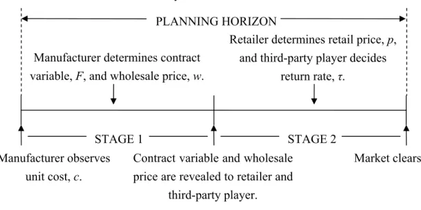
The sequence of decision-making of associated players is depicted in Figure 3. After observing the unit manufacturing cost, the manufacturer determines the wholesale price, w ,

and the contract variable, F . Then the retailer decides the retail price, p, and the third-party player determines the return rate, τ, simultaneously based on the wholesale price and the contract information revealed by the manufacturer.

Figure 3: The Timeline of the Current Recycling Model

STAGE 1 STAGE 2

PLANNING HORIZON Manufacturer determines contract

variable, F, and wholesale price, w.

Retailer determines retail price, p,

and third-party player decides return rate, τ.

Manufacturer observes unit cost, c.

Contract variable and wholesale price are revealed to retailer and

third-party player.

(21)

In practice, the manufacturer who is the first mover in decision timeline has sufficient bargaining power to act as a Stackelberg leader. When making decisions, the manufacturer considers the retailer’s and the third-party player’s best responses to its decisions. The retailer and the third-party player, making decision after observing the manufacturer’s decision, act as followers in the model. We solve this two-stage sequential game by using backward induction moving from the second stage, retailer and third-party player’s decisions, to manufacturer’s decision problem in the first stage.

Step 1. The retailer’s decision in the second stage:

The retailer maximizes its profits from selling new products as shown in (4.4). Max ( - )( - )C R p Π = φ p p w (4.4) Because 2 2 -2 0 C R d dp Π _{= < ,} C R

Π is concave in p. Then (4.4) is maximized when first-order conditions hold. From the first-order conditions, the retailer sets the retail price as

*

2 w

p =φ+ . (4.5)

Step 2. The third-party player’s decision in the second stage:

The profits of the third-party player are the income from those recycling services and the contract minus the collection effort as shown in (4.6).

* 2

3

Max ( -C )

-P A p F CL

τ Π = τ φ + τ τ (4.6)

From the second-order conditions, we have

2 3 2 -2 0 C P L d C dτ Π = < . Then 3 C P Π is

concave in τ whenever C_L > , so (4.6) is maximized when the first-order conditions hold. 0 By using the first-order conditions to derive the best response to the return rate, it gives

* ( - ) 2 _L 2 _L A p F C C φ τ = + . (4.7)

(22)

For any value of p, the third-party player determines the return rate as above. In Stage 2, the retailer or the third-party player solves its problem simultaneously. Then we substitute (4.5), the optimal retail price, into (4.7) to obtain the optimal return rate as follows:

* ( - ) 4 L 2 L A w F C C φ τ = + . _(4.8)

The profit function of third-party player, 3

C P

Π , is concave in τ . In order to ensure that the optimal return rate, _τ*_{, is bounded between zero and one, we impose the condition of}

3 1 0 C P τ τ ₌ ∂Π _<

∂ on τ . From this condition follows Assumption 1.

Assumption 1 The parameter, C , defined in the collection effort is assumed to be _L

sufficiently large such that _τ*_<₁_{, i.e.,} 2

16CL >(b A+ ) +(φ+c b A)( + ).

Step 3. The manufacturer’s decision in the first stage:

The manufacturer solves the problem to maximize its total profit which is the sum of the revenue from selling new products and those recycled hardware minus the cost on the contract relationship with the third-party player.

* * * *

,

Max ( -C )( - ) ( - )

-M

w F Π = φ p w c +bτ φ p Fτ (4.9)

When making the decision, the manufacturer would consider the retailer’s and the third-party player’s best responses to its decisions. Substituting (4.5) and (4.8) into the manufacturer’s profit function, we have

, ( - )( - ) ( - ) ( - ) Max [ ] 2 2 4 2 C M w F L L w w c b w A w F C C φ φ φ Π = + + , Max - [ ( - ) ] 4 2 D L M L w F A w F F C C φ ₊ Π = . (4.10)

(23)

To ensure C M

Π is concave in w and F , the Hessian Matrix of (4.10), -( - ) -1 4 4 -( - ) -1 4 L L L L bA b A C C b A C C ⎡ ₊ ⎤ ⎢ ⎥ ⎢ ⎥ ⎢ ⎥ ⎢ ⎥ ⎣ ⎦

, must be negative semidefinite. Then it should satisfy the conditions,

-1 0 L bA C + < , 1 0 L C − _< , and ₁₆ ₍ ₎2 L

C > b A+ . Note that C_L > then 0 1 0

L

C − _<

is trivially satisfied. According to Assumption 1, 2

16CL>(b A+ ) + +(φ c b A)( + ), and the condition, (b A+ )(φ+c) 0> , we can verify that ₁₆ ₍ ₎2

L

C > b A+ and it also implies -1 0

L

bA C

+ < .

Then the manufacturer’s profit function, C M

Π , is concave in w and F , so (4.10) is maximized when first-order conditions hold. We take the partial derivative of C

M

Π with respect to w and F as shown below:

- - ( - ) ( - ) - - -2 2 4 4 C M L L d w w c b A F bA w dw C C φ φ Π ₌ , (4.11) ( - )( - ) -4 C M L L d b A w F dF C C φ Π ₌ . (4.12)

From the first-order conditions, the manufacturer decides the wholesale price w and

the contract variable F as follows:

* * _-2 ( - ) ( - ) 4 -L L C c F b A w C bA φ φ + = (4.13) and * * ( - )( - ) 4 b A w F = φ . (4.14)

Solving the two equations for two unknown variables, the final results of w and F, which simultaneously satisfy the first-order conditions, are

* 2 8 ( - ) -16 - ( ) L L C c w C b A φ φ = + , (4.15) * 2 2 ( - )( - ) 16 - ( ) L L C c b A F C b A φ = + . (4.16)

(24)

Substituting the optimal wholesale price *

w and the contact variable _{F in (4.10), the}*

manufacturer’s profits are given by

2 * 2 2 ( - ) 16 - ( ) C L M L C c C b A φ Π = + . (4.17)

The optimal unit market price and return rate can be obtained by substituting the _w*

and _{F into (4.5) and (4.8). The total profits of the current practice model can be easily}*

found by summing up profits of the manufacturer, the retailer, and the third-party player. However, a closed-loop channel with collection in retailers is the most efficient model in Savaskan et al. (2004). Savaskan et al. (2004) investigate the recycling systems with products remanufacturing. In the retailer collection model, the retailer collects those returned products and sells them back to the manufacturer for remanufacturing processes. We integrate this concept of collection in retailers into the current practices. Then, we develop a model where the retailer engages in returned products collection to improve the current practice. In this retailer collection model, the retailer collects those obsolete products returned by customers. The manufacturer cooperates with a third-party firm to handle those recycled products which are collected by the retailer. We analyze the retailer collection model in the next section.

4.3 Retailer Collection Model

In order to make performances of recycling operations more efficient, we develop a model in this section. According to Savaskan et al. (2004), a closed-loop supply chain with the retailer engaging in collection effort is the most efficient in terms of the profits of manufacturer, the total profits, and the return rate, but recycling models with products remanufacturing do not suit for IT industry. In this section, we develop a model where the retailer collects used products with charging a service fee and the manufacturer cooperates with a third-party player. However, sometimes the retailer does not have enough ability to handle obsolete products. Then those returned products are sold to a third-party firm for

(25)

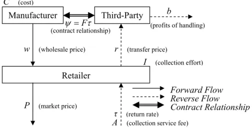
further appropriate recycled processes. The third-party player makes some profits by handling those used products collected by retailers. Figure 4 depicts this closed-loop model.

Figure 4: The Retailer Collection Model

We let r denote the revenue for the retailer from selling a unit of those used products to the third-party player. In other words, r is the unit cost of the third-party player for buying those used products from retailers. We assume that the retailer’s profits from collecting used products are positive so the condition, r A+ > , holds. The profit function 0 for member j is denoted by Π_j, where subscript j takes value M, R, or 3P, which

denotes the manufacturer, the retailer, or the third-party player, respectively. Then the profit functions of each participant are

( )( ) -M φ p w c Fτ Π = , (4.18) 2 ( - )( - ) ( )( ) -R φ p p w τ r A φ p CLτ Π = + + , (4.19) 3P τ( - )( - )b r φ p Fτ Π = + . (4.20) τ (return rate) Manufacturer Third-Party Retailer Reverse Flow Forward Flow F ψ = τ Contract Relationship w (wholesale price) P (market price) C (cost) I (collection effort) b

A (collection service fee)

r (transfer price)

(profits of handling) (contract relationship)

(26)

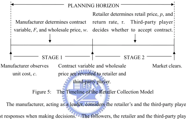
The sequence of decision-making in this supply chain channel is shown in Figure 5. After observing the unit manufacturing cost, the manufacturer determines the wholesale price,

w , and the contract variable, F. Then the retailer decides the retail price, p, and the third-party player determines the return rate, τ, simultaneously based on the wholesale price and the contract information revealed by the manufacturer.

Figure 5: The Timeline of the Retailer Collection Model

The manufacturer, acting as a leader, considers the retailer’s and the third-party player’s best responses when making decisions. The followers, the retailer and the third-party player, make decisions after observing the manufacturer’s decision. We apply the backward induction to study this sequential two-stage model moving from the retailer’s and the third-party player’s decision problems in the second stage to the manufacturer’s decision problem in the first stage.

Step 1. The retailer’s decision in the second stage:

The retailer maximizes its profit function, Π , which is the profits from selling new R

products and recycling units minus the collection effort as shown in (4.21).

2 ,

Max ( - )( - )_R ( )( - ) - _L

pτ Π = φ p p w +τ r A+ φ p C τ (4.21)

From the first-order conditions, p and * _{τ are}*

STAGE 1 STAGE 2

PLANNING HORIZON Manufacturer determines contract

variable, F, and wholesale price, w.

Manufacturer observes unit cost, c.

Contract variable and wholesale price are revealed to retailer and

third-party player.

Market clears. Retailer determines retail price, p, and

return rate, τ. Third-party player

(27)

* * - ( ) 2 w r A p =φ+ τ + , and (4.22) * * ( - )( ) 2 _L p r A C φ τ = + . (4.23)

Solving the two equations for two unknown variables, we obtain the optimal market price p and return rate * _{τ , which satisfy the first-order conditions, as follows:}*

* 2 2 ( - ) -4 - ( ) L L C w p C r A φ φ = + , (4.24) * 2 ( - )( ) 4 L- ( ) w r A C r A φ τ = + + . (4.25)

Intuitively, the return rate, τ , must be lower than one. To ensure this, we assume that retailer’s profit function is down-sloping at τ = , i.e., 1

1 0 R τ τ ₌ ∂Π _<

∂ . Then the optimal return rate which makes the retailer’s profit function be maximized is lower than one. From this condition follows Assumption 2.

Assumption 2 Parameter C defined in the collection effort is assumed to be sufficiently _L

large such that_τ* _<₁_{, i.e., which means} ( )2 ( )( - )

4

L

r A r A w C > + + + φ .

To ensure that Π is concave in _R p and τ , the Hessian Matrix of Π , _R -2 -- -- -2 _L r A r A C ⎡ ⎤ ⎢ ⎥

⎣ ⎦, must be negative semidefinite, i.e., -2CL < and 0

2 ( ) 4 L r A C > + . Note

that C is positive, so we have -2_L C_L < . From Assumptions 2, we know that 0

2

( ) ( )( - ) 4

L

r A r A w

C > + + + φ and, then, it follows

2

( ) 4

L

r A

C > + . Therefore, the retailer’s profit function is concave in p and τ , then (4.21) is maximized when the first-order conditions hold.

(28)

In this step, we investigate the third-party player’s decision. The profit function of the third-party player, which includes the profits from those obsolete products plus the revenue from the contract, is shown below.

* * *

3P τ ( - )( -b r φ p ) Fτ

Π = + (4.26)

Under our modeling setting, all of these notations in the profit function are given parameters for the third-party player. In other words, there is no decision variable in this step. Therefore, instead of maximizing its profits, the third-party player would make the decision about whether to accept the contract provided by the manufacturer or not.

The third-party player would accept the contract when its profits are positive, i.e.,

3P 0

Π ≥ . Then we have a constraint about the contract variable F for any value of pto ensure that the third-party player is with a non-negative profit.

*

-( - )( )

F ≥ b r φ−p (4.27)

In stage 2, the third-party player and the retailer make decisions simultaneously. Then we substitute (4.24) into (4.27) and get the constraint of the contract variable,

2 2 ( )( ) 4 ( ) L L C w b r F C r A φ− − ≥ − − + . (4.28)

Constraint (4.28) shows that there exists a lower bound of F, which is the decision variable of the manufacturer. It implies that the contract must be attractive enough to the third-party player so that the third-party player has incentives to accept the contract. From (4.28), we know that the lower bound of F is positive whenever r b> . It means that if the unit cost of those obsolete products is higher than the unit revenue, the manufacturer would pay the third-party player to help it take the responsibility of the recycling processes. On the contrary, if the third-party player can receive positive profits from those used products, it has incentives to join this closed-loop supply chain collection program without any payment from the manufacturer.

(29)

Step 3. The manufacturer’s decision in the first stage:

The manufacturer decides the wholesale price, w , and the contract, F, to maximize its profits from selling the new products minus the cost of contract as below.

* *

,

Max ( -_M )( )

-w F Π = φ p w c Fτ (4.29)

When making the decision, the manufacturer would consider the retailer’s and the third-party player’s best responses. Substituting (4.24) and (4.25) into this profit function, we have 2 2 , 2 ( - )( - ) ( - )( ) Max -4 - ( ) 4 - ( ) L M w F L L C w w c F w r A C r A C r A φ φ + Π = + + . (4.30)

Lemma 1 The profit of the manufacturer is maximized when F reaches the lower bound. Proof. We let F denote the lower bound of F. Assuming that there exists a F'= + F ε

where ε > , such that the profits of the manufacturer is maximized, i.e., 0 _{( )}' _{( )}

M F M F

Π > Π .

Then, we have an inequality, -( - )( ₂) 0

4 L- ( )

w r A

C r A

φ + _ε _>

+ . Assumptions 2 and condition, ( - ) 0φ w > , contract this inequality. Therefore, the profits of the manufacturer is maximized while the contract variable, F, reaches its lower bound. ■

Lemma 1 simplifies the manufacturer’s problem into a single-variable problem. Substituting the lower bound of the contact variable, F , into (4.30), then we have

2 2 2 2 2 ( - )( - ) 2 ( - ) ( - )( ) Max 4 - ( ) [4 - ( ) ] L L M w L L C w w c C w b r r A C r A C r A φ φ + Π = + + + . (4.31)

From the first-order conditions, the optimal wholesale price is

2 * _-( - )[4 - ( ) ] 8 - 2( )( ) L L c C r A w C r A b A φ φ + = + + . (4.32)

The second-order conditions,

2 2 0 M d dw Π _< , hold whenever ₄_CL_{≥ +}₍_{r A}₎2 (r A b r)( - )

+ + . Substituting (4.32) into the constraint from Assumption 2,

2 ( ) ( )( - ) 4 L r A r A w C > + + + φ , we have ₄ ₍ ₎2 ₍ _{)( - )} ( )( - ) 2 L r A c C > +r A + +r A b r + + φ .

(30)

2

2 0

M

d dw

Π _{< , hold. Then, the profit function of the manufacturer is concave in w so (4.31)} is maximized when the first-order conditions hold. Finally, the manufacturer’s profit is given by 2 * ( - ) 8 - 2( )( ) L M L C c C r A b A φ Π = + + . (4.33)

The optimal return rate can be found by substitution of _w*_{, then we have} * ( )( - ) ( - ) 8 8 - 2( )( ) _{- 2(} ₎ ( ) L L r A c c C C r A b A _{b A} r A φ φ τ = + = + + ₊ + . (4.34)

From (4.33) and (4.34), we find that the optimal return rate, _τ*_{, is positively related to}

r and the profits of the manufacturer, Π , are also positively related to _M r. Therefore, the profits of the manufacturer, Π , are positively related to the return rate, _M τ . Then the manufacturer would like to see a high products return rate.

Proposition 1 The manufacturer would like to provide the third-party player with an

appropriate contract, which induce the retailer to increase the return rate.

Proof. From Lemma 1, the optimal contract variable, F, which reaches its lower bound,

( )( ) 4 ( )( ) L L C c r b C r A b A φ− −

− + + , is a function of r . Moreover, the optimal return rate,

* ( )( - ) 8 _L- 2( )( ) r A c C r A b A φ τ = +

+ + , is also a function of r. Then the manufacturer could control r

indirectly by offering the third-party player an appropriate contract so that it can affect the retailer’s decision, the return rate, τ. Furthermore, the profits of the manufacturer, Π , _M are positively related to the return rate, τ . In order to maximize its profits, the manufacturer would determine an appropriate contract to induce the retailer to increase the return rate, τ . ■

In the next section, we summarize all decision variables and profit functions of the two proposed models, the retailer collection model and the current practice model. We compare

(31)

the return rates, the profits of manufacturer, and the total profits between these two models. Then we investigate the performance comparison when the third-party player is a non-profit organization. We conduct sensitivity analysis to study some interesting issues about the collection effort parameter, C , and some interactions between parameters, _L C , _L b, r, and

(32)

Chapter 5. Comparison of Two Recycling Systems

In this section, we draw some managerial insights related to the return rates, the profits of manufacturer, and the total profits for comparison of the current recycling practice model and the retailer collection model. We consider the third-party player in the retailer collection model acting as a non-profit organization who considers the fund balance between unit cost and unit revenue instead of the profit-maximization objective. Then we study the effect by alternating the collection effort, the recycling service fee, the revenue from treated obsolete products, and the payment of the third-party player to purchase returned products from the retailer.

5.1 Performance Comparison

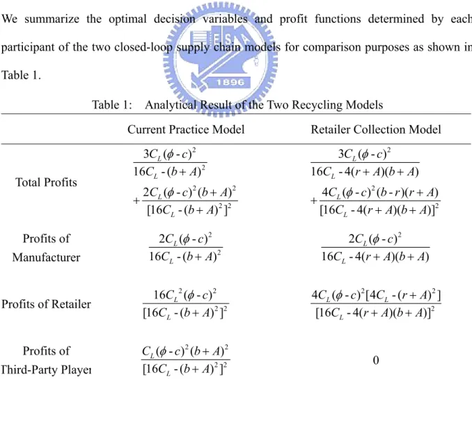
We summarize the optimal decision variables and profit functions determined by each participant of the two closed-loop supply chain models for comparison purposes as shown in Table 1.

Table 1: Analytical Result of the Two Recycling Models

Current Practice Model Retailer Collection Model

Total Profits 2 2 2 2 2 2 3 ( - ) 16 - ( ) 2 ( - ) ( ) [16 - ( ) ] L L L L C c C b A C c b A C b A φ φ + + + + 2 2 2 3 ( - ) 16 - 4( )( ) 4 ( - ) ( - )( ) [16 - 4( )( )] L L L L C c C r A b A C c b r r A C r A b A φ φ + + + + + + Profits of Manufacturer 2 2 2 ( - ) 16 - ( ) L L C c C b A φ + 2 2 ( - ) 16 - 4( )( ) L L C c C r A b A φ + + Profits of Retailer 2 2 2 2 16 ( - ) [16 - ( ) ] L L C c C b A φ + 2 2 2 4 ( - ) [4 - ( ) ] [16 - 4( )( )] L L L C c C r A C r A b A φ + + + Profits of Third-Party Player 2 2 2 2 ( - ) ( ) [16 - ( ) ] L L C c b A C b A φ + + 0

(33)

Market Price 2 4 ( - ) -16 - ( ) L L C c C b A φ φ + 4 ( - ) -16 - 4( )( ) L L C c C r A b A φ φ + + Wholesale Price 2 8 ( - ) -16 - ( ) L L C c C b A φ φ + 2 2( - )[4 - ( ) ] -16 - 4( )( ) L L c C r A C r A b A φ φ + + + Return Rate 2 ( - )( ) 16 _L- ( ) c b A C b A φ + + 2( - )( ) 16 _L- 4( )( ) c r A C r A b A φ + + + Contract Variable 2 2 ( - )( ) 16 - ( ) L L C c b A C b A φ − + 4 ( - )( ) 16 - 4( )( ) L L C c b r C r A b A φ − − + +

We evaluate the effect of recycling systems from different aspects of the return rates, the profits of the manufacturer, and the total profits. A rational player in recycling systems would like to increase its profits. The manufacturer who is the first mover in closed-loop supply chains has the most bargaining power and it is reasonable assuming that the manufacturer is seeking the maximum of its profits. However, in the perspective of the system designer, the return rate and the total profits are two important performance indicators in recycling systems. In this study, we are also interested in the trend of the return rate and total profits in the system designer’s perspective. Therefore, we compare these performance measures in terms of the return rates, the manufacturer’s profits, and the total profits between the current recycling system and the retailer collection model.

Observation 1 The optimal return rate in the retailer collection model, τ , is greater than *

the optimal return rate in the current practice model, _{τ , whenever the condition}C* 2

32C r AL( + ) -16C b AL( + ) 2(+ r A b A+ )( + ) >0 holds.

Proof. The condition, 32C r A_L( + ) -16C b A_L( + ) 2(+ r A b A+ )( + )2 >0, can be written as

2 8 ( ) 16 ( ) L L C b A r A C b A + > −

+ + . Note that, in the retailer collection model, the retailer’s profits from

collecting obsolete products are τ⋅ +(r A)(φ−p). In the current practice, the third-party player earns A⋅τ φ( −p)+ ⋅F τ from returned products. In the retailer collection model, the

(34)

retailer’s profits from collection work would be increased when the third-party player provides more payment to the retailer for those returned products. Therefore, the retailer would determine the return rate which is higher than the return rate in the current practices model when r is large enough. More specifically, 8 ( ) ₂

16 ( ) L L C b A r A C b A + > − + + . ■

Observation 2 The optimal profits of the manufacturer in the retailer collection model are

high than the profits in the current practice, i.e., C

M M

Π > Π , whenever the condition

4(r A+ ) (> b A+ ) holds.

Proof. From Table 1, we observe that the profits of the manufacturer in the retailer

collection model increase with r. The manufacturer’s profits in the retailer collection model would be greater than the profits of the manufacturer in the current practice whenever

4 b A

r> + −A. In the retailer collection model, when the retailer’s unit revenue from returned products, r, increases, it gives the retailer incentives to increase the quantity of recycled products. The quantity of recycled products, τ φ⋅( - )p , is positively related to the return rate and the market demands of new products. The profits of the manufacturer are also positively related to the market demands of new products. Then in the retailer collection model, the manufacturer can earn more profits with more recycled products as r

increases. Therefore, when r is large enough, i.e.,

4 b A

r> + −A, the manufacturer’s profits in the retailer collection model would be higher than the profits of manufacturer in the current practice model. ■

Finally, we compare the total profits between the retailer collection model and the current practice model. The unit payment between the retailer and the third-party player, r, is not a market parameter so it can be negotiated by the players in the retailer collection model. We study how the change in the total profits as parameter, r, changes. From Assumption 2, we know that there exists an upper bound of r, 8CL

2( ) ( )

r A

b A φ c

< −

(35)

condition, r A+ >0, we have the lower bound of r. Then we observe the total profit functions within the feasible region of r. In the current practice, the total profits, C

T

Π , are fixed with different r. Then we observe variation of the total profits in the retailer collection model, Π , and compare it with the total profits in the current practice model. _T However, from the second-order conditions, the concavity of Π is undetermined when _T parameter settings vary. In this study, we use two numerical examples to demonstrate different types of the total profit function, Π , which is affected by the unit payment from _T the third-party player to the retailer, r.

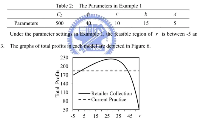
Example 1 The parameters, C , _L φ , c , b , and A, are given in Table 2.

Table 2: The Parameters in Example 1

CL φ c b A

Parameters 500 40 10 15 5

Under the parameter settings in Example 1, the feasible region of r is between -5 and 53. The graphs of total profits in each model are depicted in Figure 6.

Figure 6: Graphs of Total Profits under Example 1

When b is lower than the upper bound of r, i.e., 15 53< , the total profit function in the retailer collection model is not monotonic increasing within the feasible region of r. Then the total profits in the retailer collection model would not always be higher than that in the current practice model. In Example 1, the total profits in the retailer collection model would be higher than the total profits in the current practice model whenever r falls within

50 80 110 140 170 200 230 -5 5 15 25 35 45 To tal Prof its r Retailer Collection Current Practice

(36)

1.76 to 43.12. From Table 1, the term, (b r− ), of the total profits in the retailer collection model would be negative whenever r b> . Therefore, the total profits in the retailer collection model would be lower than the total profits in the current practice model when r

still increases.

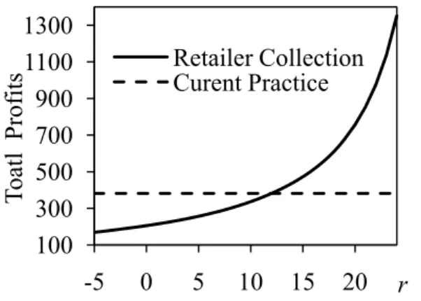
Example 2 The parameters, C , _L φ , c , b , and A, are given in Table 3.

Table 3: The Parameters in Example 2

CL φ c b A

Parameters 500 40 10 50 5

Under this parameter settings in Example 2, the feasible region of r is between -5 and 24. The graphs of total profits in each model are depicted in Figure 7.

Figure 7: Graphs of Total Profits under Example 2

When b exceeds the feasible region of r, i.e., 50 24> , the total profit function of the retailer collection model is an increasing function within the feasible region of r. When r

is large, i.e., r>12.02 in this example, the total profits of the retailer collection model would be higher than that in the current practice model.

5.2 A Special Case – Non-Profit Third-Party

With the increase of the environmental consciousness, some non-government organizations (NGOs) engage in obsolete products return markets. Many of these NGOs are non-profit organizations. In Switzerland, there were four non-profit organizations managing the financing, collection, transportation, and control systems for electronics industry in 2007

100 300 500 700 900 1100 1300 -5 0 5 10 15 20 To atl Prof its r Retailer Collection Curent Practice

(37)

(Khetriwal et al. 2009). Then we are interested in drawing the practice of non-profit organizations into the retailer collection model.

It is reasonable to view the third-party player in the retailer collection model as a role of non-profit organizations. The third-party player’s profits from returned products are

(b r)( p)

τ⋅ − φ− . Acting as a non-profit organization, the third-party player would not seek its profits maximized; in other words, the cost of those obsolete products, r⋅ ⋅ −τ φ( p), is equal to the revenue, b⋅ ⋅ −τ φ( p). Then the unit cost, r , is equal to the unit revenue, b .

Therefore, we set r b= in the retailer collection model. The optimal return rate, the profits of the manufacturer, and the total profits can be obtained by substituting r b= into the results of the retailer collection model in Table 1. Then we have

2 2( - )( ) 16 _L 4( ) c b A C b A φ τ = + − + , (5.1) 2 2 ( ) 16 4( ) L M L C c C b A φ− Π = − + , (5.2) 2 2 3 ( ) 16 4( ) L T L C c C b A φ− Π = − + . (5.3)

These results give us more interesting insights. We compare these performances with the results of the current practice model. From Observation 1, the condition,

2

32C r AL( + ) -16C b AL( + ) 2(+ r A b A+ )( + ) >0, can be rewritten as

2

16CL+2(b A+ ) >0.

It is trivial to show that ₁₆ ₂₍ ₎2

L

C + b A+ is greater than zero because C and _L ₍_{b A}₊ ₎2_are

both positive. Then the optimal return rate, τ , is greater than the current return rate, _{τ .}C

The condition in Observation 2, 4(r A+ ) (> b A+ ), holds whenever r is equal to b . Therefore, we have C

M M

Π > Π whenever r b= . We compute the term C

T T

Π − Π to

compare the total profits between these two models. The total profits in the retailer collection model are greater than the profits in the current practice model when the condition

2

112CL− +(b A) >0 holds. From Assumption 2, we have

2

(38)

r b= so the condition, 2

112CL− +(b A) >0, holds. Then the total profits in retailer

collection model, Π , are greater than that in the current practice, _T C T

Π . Therefore, when the third-party player is viewed as a non-profit organization, the proposed model where the retailer engages in collection effort outperforms the current practice model where the third-party player collects returned products in terms of the return rate, manufacturer’s profits and total profits.

5.3 Sensitivity Analysis

In this section, we describe the numerical studies that examine the return rates and profits of manufacturer of the proposed recycling models. We examine return rates and profits of the manufacturer in each recycling model by adjusting parameters, C , _L A, r, and b. The difference between the two proposed models is that the retailer collects those used products in the retailer collection model but those used products are collected by the third-party player in the current practice model. Then we are interested in the effect of different collection efforts on the return rate and the profits of manufacturer between the retailer and the third-party player. We also examine the performance measures in the two proposed models by taking into account some parameters such as C , _L A, r and b.

In the retailer collection model, those obsolete products are collected by the retailer instead of the third-party player who collects used products in the current recycling system. Then we conduct sensitivity analysis to examine the performance of each recycling model when the collection effort parameters, C , are different between the retailer and the _L

third-party player. Other parameters are given in Table 4 where C L

C denotes the collection effort parameter in the current practice model.

(39)

Table 4: Parameters in Sensitivity Analysis of CL

CLC φ c b A r

200 40 10 15 5 15 We vary the values for collection effort parameter, C , in the retailer collection model _L

from 180 to 580 which are 0.9 to 2.9 times of C L

C when the collection effort parameter in the current practice model, C

L

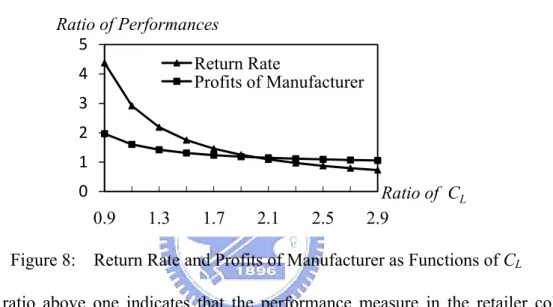
C , remains the same level. The results of the return rates and the profits of the manufacturer are depicted in Figure 8.

Figure 8: Return Rate and Profits of Manufacturer as Functions of CL

The ratio above one indicates that the performance measure in the retailer collection model is higher than that in the current practice model. The collection effort, 2

L

I =C ⋅τ , is the cost paid by the associated party who engages in collecting those returned products. An increase in C means that it is more costly to increase the return rate. As the collection _L

cost of the retailer, C , increases, the return rate and the profits of manufacturer in the _L

retailer collection model decrease, even lower than the return rate and the profits of manufacturer in the current practice model. In this parameter setting, the return rate in the retailer collection model would be lower than that in the current practice model when the collection effort of the retailer is more than the third-party player’s collection effort about 2.5

0 1 2 3 4 5 0.9 1.3 1.7 2.1 2.5 2.9 Return Rate Profits of Manufacturer Ratio of Performances Ratio of C_L

(40)

times and the ratio of manufacturer’s profit would be lower than one when the ratio of C is _L

over 2.9.

We also conduct sensitivity analysis to examine the performance measures affected by the collection effort parameter, C , and the collection service fee, A . Parameters are given _L

in Table 5.

Table 5: Parameters in Sensitivity Analysis of CL and A

CLC φ c b r

200 40 10 15 15

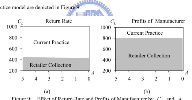
We consider the values for collection service fee, A, from five to zero and the collection effort of the retailer, C_L, from 200 to 1000. Then the relationship of the return rate and the profits of manufacturer between the retailer collection model and the current practice model are depicted in Figure 9.

(a) (b)

Figure 9: Effect of Return Rate and Profits of Manufacturer by C and _L A

The return rate in the retailer collection model is better than that in the current practice model when the ratio of C and _L A are in the lower region of Figure 9(a). The manufacturer earns more profits in the retailer collection model than in the current practice model with any value of the collection service fee, A, when the ratio of C is less than _L

four. 200 400 600 800 1000 5 4 3 2 1 0A CL Return Rate Retailer Collection Current Practice 200 400 600 800 1000 5 4 3 2 1 0A CL Profits of Manufacturer Retailer Collection Current Practice

(41)

Then we examine the interaction effect of the collection service fee, A, and the unit payment from the third-party player to the retailer in the retailer collection model, r, on the return rate and the profits of manufacturer. Other parameters are given in Table 6.

Table 6: Parameters in Sensitivity Analysis of r and A

CL φ c b

500 40 10 15

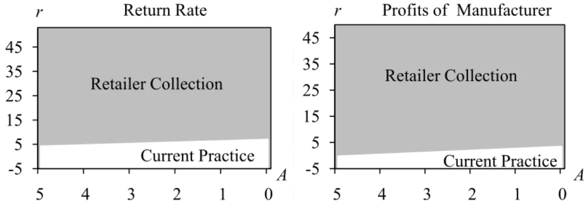
We vary the values for collection service fee, A, from five to zero and the payment from the third-party player to the retailer , r, from -5 to 50. Then the comparison results of the return rate and the profits of manufacturer between the retailer collection model and the current practice model are depicted in Figure 10.

Figure 10: Effect of Return Rate and Profits of Manufacturer by r and A

The retailer collection model acts better performances than the current practice model as

r and A both increase. In the retailer collection model, the retailer has more incentive to collect obsolete products with a higher service fee or a higher unit payment from the third-party player. If r and A are in low levels, the retailer may not pay much attention on the collection work.

We also conduct sensitivity analysis for both, b and r, which are the unit revenue and cost from handling those returned products, to examine the return rate and the profits of manufacturer. Other parameters are given in Table 7.

-5 5 15 25 35 45 5 4 3 2 1 0A r Return Rate Retailer Collection Current Practice -5 5 15 25 35 45 5 4 3 2 1 0 A r Profits of Manufacturer Retailer Collection Current Practice

(42)

Table 7: Parameters in Sensitivity Analysis of r and b

CL φ c A

500 40 10 5

We vary the values of b from 10 to 15 and the values of r from -5 to 50. Then we depict the comparison results of the return rate and the profits of manufacturer between the retailer collection model and the current practice model in Figure 11.

Figure 11: Effect of Return Rate and Profits of Manufacturer by r and b

As the unit revenue from handling those returned products, b, increases, the return rate and the profits of manufacturer would increase in both proposed recycling models. From Figure 11, as b increases, we find that the current practice model acts better performances in a large range of r compared to the retailer collection model. Therefore, the effect of the parameter, b, in the current practice model is larger than in the retailer collection model. We summarize some conclusions and future research in the next section.

-5 5 15 25 35 45 10 11 12 13 14 15 b r Return Rate Retailer Collection Current Practice -5 5 15 25 35 45 10 11 12 13 14 15 b r Profits of Manufacturer Retailer Collection Current Practice