基於長期感測雜訊變異量消息之無線感測網路能量效率化分散式估計

基於長期感測雜訊變異量消息之無線感測網路

能量效率化分散式估計

學生：黃千致

指導教授：李大嵩 博士

國立交通大學電信工程學系碩士班

摘要

在無線感測網路中因頻寬與能量的限制，每個感測器只能傳送有限個位元數 至 融 合 中 心 ， 此 融 合 中 心 接 收 資 料 並 且 利 用 最 佳 線 性 不 偏 估 計 (best-linear-unbiased-estimator)融合規則估計未知參數。本論文中有兩種最 佳能量分配策略被考慮：最小能量分散式估計及最小均方誤差(minimal mean square error)分散式估計。第一種策略為最小化總能量並滿足某程度的效能限 制，而此效能限制為對量測雜訊變異量機率分佈取平均後的均方誤差。第二種策 略為最小化平均均方誤差並滿足某程度的總能量限制。我們也考慮最小能量分散 式估計在路徑衰減的拉瑞衰減通道中，而這個感測器與融合中心之間的通道用二 進位對稱式通道(binary symmetric channel)來表示。現今有關能量分配的相關 研究皆需已知瞬間雜訊變異量，而本論文提出的演算法只需知道長期雜訊變異量 的統計特性。而這個問題被表示成凸型最佳化問題(convex optimization)，並 且得到封閉式最佳解，最後從此演算法中可以發現一些與其他相關研究共同的特 性。根據模擬結果，此演算法確實能顯著的改進能量使用效率比起均衡式能量分 配。

Energy-efficient Decentralized Estimation in

Wireless Sensor Network Based on Long-Term

Noise Variance Knowledge

Student:

Qian-Zhi

Huang

Advisor:

Dr.

Ta-Sung

Lee

Department of Communication Engineering

National Chiao Tung University

Abstract

In a wireless sensor network, due to bandwidth and energy limitation, each sensor is only able to transmit a finite number of bits to the fusion center (FC) which combines the received bits to estimate the unknown parameter by the best-linear-unbiased-estimator (BLUE) fusion rule. In this thesis, the optimal power allocation strategies are considered for two cases: minimal energy decentralized estimation and minimal mean square error decentralized estimation. In the first case, the minimization of total energy is subject to a certain performance constraint in terms of mean square error (MSE) averaged over the noise variance distribution. In the second case, the minimization of the average MSE is subject to a certain energy constraint. We also consider the minimal energy decentralized estimation over rayleigh fading channels with path loss. The wireless links between sensors and the FC are characterized by the binary symmetric channels (BSCs). While most of the existing related works require the knowledge of instantaneous noise variance for energy allocation, the proposed approach instead relies on an associated model. The problems can be reformulated in the form of convex optimization and the closed-form optimal solutions are obtained. The proposed schemes share several attractive features of the existing designs and are seen to significantly improve energy efficiency against the uniform allocation schemes by the simulation results.

Acknowledgement

I would like to express my deepest gratitude to my advisor, Dr. Ta-Sung Lee, for his enthusiastic guidance and great patience. I learn a lot from his positive attitude in many areas. Heartfelt thanks are also offered to all members in the Communication System Design and Signal Processing (CSDSP) Lab for their constant encouragement. Finally, I would like to show my sincere thanks to my parents for their invaluable love.

Contents

Chinese Abstract

………..

I

English Abstract

……….

II

Acknowledgement

...

III

Contents

...

IV

List of Figures

...

VI

Acronym Glossary

...

VII

Chapter 1 Introduction ...1

Chapter 2 Wireless Sensor Network Overview ...4

2.1 System Model of Wireless Sensor Networks...5

2.2 Decentralized Estimation Scheme (DES) ...8

2.3 Mean Square Error (MSE) of Decentralized Estimation ...9

Chapter 3 Minimal Energy Decentralized Estimation Based on Sensor

Noise Variance Statistics...11

3.1 Average Mean Square Error of Decentralized Estimation ...12

3.2 Energy Density Factor of Sensor Nodes ...15

3.3 Problem Formulation and Optimal Closed-form Solution...16

3.4 Discussions of Optimal Solution ...18

3.5 Numerical Simulation ...20

3.6 Summary ...22

Chapter 4 Minimal Mean Square Error Decentralized Estimation Based on

Sensor Noise Variance Statistics...23

4.1 Average Mean Square Error of Decentralized Estimation ...24

4.3 Problem Formulation and Optimal Closed-form Solution...28

4.4 Discussions of Optimal Solution ...30

4.5 Numerical Simulation ...32

4.6 Summary ...34

Chapter 5 Minimal Energy Decentralized Estimation over Rayleigh Fading

Channel Based on Sensor Noise Variance Statistics...35

5.1 System Model ...37

5.2 Variance of Distortion in Binary Symmetric Channel (BSC) ...39

5.3 Average Bit Error Rate (BER) in BSC Mode over Rayleigh Fading Channel with Path Loss...40

5.4 Average Mean Square Error of Decentralized Estimation ...42

5.5 Problem Formulation and Suboptimal Closed-form Solution ...46

5.6 Discussions of Suboptimal Solution ...48

5.7 Numerical Simulation ...50

5.8 Summary ...52

Chapter 6 Conclusion...54

Appendix...57

List of Figures

Figure 2.1 : System Model of Wireless Sensor Network...5 Figure 3.1 : PES for fixed minimal noise variance threshold (δ =0.8) ...21 Figure 3.2 : PES for fixed noise variance variation (α =0.4) ...22 Figure 4.1 : Average MSE for fixed minimal noise variance threshold (δ = ) ...33 2 Figure 4.2 : Average MSE for fixed noise variance variation (α = )...34 2 Figure 5.1 : Binary symmetric channel...38 Figure 5.2 : PES for fixed minimal noise variance threshold (δ =0.85) ...51 Figure 5.3 : PES for fixed noise variance variation (α =1.45) ...52

Acronym Glossary

AWGN additive white Gaussian noise

BER bit error rate

BSC binary symmetric channel BPSK binary phase shift keying BLUE best linear unbiased estimator CSI channel state information

DES decentralized estimation schemes

FC fusion center

IEEE institute of electrical and electronics engineers ISI intersymbol interference

KKT Karush-Kuhn-Tucker

LB lower bound

LOS line of sight

MMSE minimum mean square error MSE mean square error

PES percentage of energy saving

PHY physical layer

PDF probability density function QAM quadrature amplitude modulation QPSK quaternary phase shift keying RX receiver

SNR signal-to-noise ratio TX transmitter

Chapter 1

Equation Chapter 1 Section 1

Introduction

Wireless sensor networks (WSNs) are ideal for environmental monitoring applications because of their low implementation cost, agility, and robustness to sensor failures. A popular WSN architecture consists of a fusion center (FC) and a large number of spatially distributed sensors. The FC can be either a standard base station or a mobile access point such as an unmanned aerial vehicle hovering over the sensor field. Each sensor in a WSN is responsible for local data collection as well as occasional transmission of a summary of its observations to the FC via a wireless link. In a practical WSN, each sensor has only limited computation and communication capabilities due to various design considerations such as small size battery, bandwidth, and cost.

As a result, it is difficult for sensors to send their entire real-valued observations to the FC. Instead, a more practical decentralized estimation scheme is to let each sensor quantize its real-valued local measurement to an appropriate length and send the resulting discrete message (typically short) to the FC, while the latter combines all the received messages to produce a final estimate of the unknown parameter. Naturally, the message lengths are dictated by the power and bandwidth limitations,

sensor noise characteristics, wireless channel condition as well as the desired final estimation accuracy.

Recently, several decentralized estimation schemes (DES) [1, 2, 3] have been proposed for parameter estimation in the presence of additive sensor noise. These DESs require each sensor to send only a few bits to the fusion center, with the message length determined by the sensor’s local SNR. Performance of the resulting estimator is shown to be within a constant factor of the best linear unbiased estimator (BLUE) performance.

In a practical WSN, the wireless links from sensors to the FC may have different qualities, depending on the sensor locations relative to the FC. Intuitively, local message length should depend not only on the quality of sensor’s observation (i.e., local SNR), but also on the quality of its wireless link to the FC. In particular, even if a sensor has a high quality observation, it should not perform any local quantization or transmission when its wireless link to the FC is weak, in order to conserve sensor energy. In general, minimizing the total sensor energy consumption for a decentralized estimation task is essential to ensure long lifespan of a WSN. Motivated by these considerations, the authors of [4, 5] proposed optimal coded and uncoded transmission strategies for sensor networks which can minimize the required energy per transmitted bit, although no consideration was given to the quantization effect and the accuracy of final estimation.

As energy efficiency is a critical concern for sensor network design [6, 7, 8], the decentralized estimation is formulated as optimal bit-loading problem. In the practical system the probability density function (pdf) of the observation noise is hard to characterize, especially for a large scale sensor network. The signal processing algorithms that do not require knowledge of the sensor noise pdf have been proposed

instantaneous noise variances for energy allocation, the proposed approach instead relies on an associated statistical model. In order to improve the estimation performance against the variation of sensing conditions, repeated update of the noise profile would be needed. This comes inevitably at the cost of more training overhead and extra energy consumption. If the sensing environment is harsh, the sensing noise will change quickly. The proposed signal processing algorithm which relies on an associated sensing noise variance model is needed

This thesis is organized as follows. In Chapter 2, we introduce the system model of wireless sensor networks and decentralized estimation scheme. In Chapter 3, minimal energy decentralized estimation based on long-term noise variance knowledge is proposed. In Chapter 4, minimal mean square error decentralized estimation based on long-term noise variance knowledge is proposed. In Chapter 5, we consider minimal energy decentralized estimation with the noisy channel between each sensor and the FC by exploiting long term noise variance information. The main results are presented and the numerical performance of the proposed schemes are illustrated. Finally, we conclude this thesis and propose some potential future works in Chapter 6.

Chapter 2

Equation Chapter (Next) Section 1

Wireless Sensor Network Overview

Recent technological advances in Wireless Sensor Networks have led to the emergence of small, inexpensive, and low-power sensor devices with limited on-board processing and communication capabilities. When suitably programmed and deployed in large scale, such networked sensors can cooperate to accomplish various high-level tasks. Sensor networks of this type are well-suited for situation awareness applications such as environmental monitoring (air, water, and soil), smart factory instrumentation, military surveillance, precision agriculture, intelligent transportation and space exploration.

WSNs deploy geographically distributed sensor nodes to collect information of interest. The collected information is then aggregated via wireless transmissions at a fusion center to generate the final intelligence. A typical wireless sensor network consists of a fusion center and a number of sensors. The sensors typically have limited energy resources and communication capability. Each sensor in the network makes an observation of the quantity of interest, generates a local signal, and then sends it to the fusion center where the received sensor signals are combined to produce a final estimate of the observed quantity.

Since sensors have only small-size batteries whose replacement can be costly, sensor network operations must be energy efficient in order to maximize network lifespan. A main objective of current sensor network research is to design energy-efficient devices and algorithms to support all aspects of network operations.

2.1 System Model of Wireless Sensor

Networks

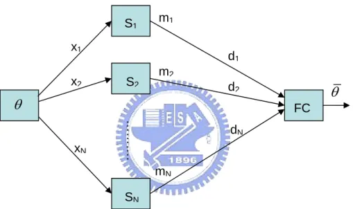
S2 S1 SN ………. x1 x2 xN m1 m2 mN d1 d2 dN FC

θ

θ

Figure 2.1 : System Model of Wireless Sensor Network

A common WSN architecture consists of a fusion center and a number of geographically distributed sensors. Such network architecture can be used to accomplish a joint signal processing task such as decentralized estimation and detection. In this chapter, we consider decentralized estimation of an unknown by a set of distributed sensor nodes and a fusion center. The sensors collect real-valued data, perform a local data compression and send the resulting discrete messages to the fusion center, while the latter combines the received messages to produce a final estimate of the observed signal.

the fusion center a short discrete message whose length is determined by the local signal-to-noise ratio (SNR), while guaranteeing a mean squared estimation error (MSE) performance that is within a constant factor of that achieved by the centralized best linear unbiased estimator (BLUE). However, this chapter still assumes that the wireless channel between sensor and fusion center are ideal without any distortion.

2.1.1 Measurement and Quantization of Each Sensor

Consider a set of N distributed sensors, each making observations on deterministic source signal θ. The observations are corrupted by additive noise. The local observation at the ith node is

, x_i = +θ n_i 1≤ ≤i N, (2.1)

where ni is zero-mean measurement noise with variance σi2. A commonly used

statistical description for sensor noise variance is [6, 7]

N (2.2) where 2 , 1 , i zi i σ = +δ α ≤ ≤

models the network-wide noise variance threshold, α

δ controls the

underlying variation from the nominal minimum, and z_i ∼χ₁2 is a central Chi-Square distributed random variable with degrees-of-freedom equal to one[10,

i

p-24]. Due to bandwidth and power limitations each sensor quantizes its observation into a b -bit message, and then transmits this locally processed data to the FC to generate a final estimate of θ. In this thesis the uniform quantization scheme with nearest-rounding [11, 12] is adopted.

The quantized message at the ith sensor can be modeled as

, m_i = +x_i q_i 1≤ ≤i N, (2.3)

here is the quantization error which is uniformly

variance 2 2 12 4 i i

b q R

σ = ⋅ [11].

[

−R 2,R 2

]

is the available signal amplitude range common to all sensors. With (2.1) and (2.3), the received data from all sensor output can be expressed in a vector form as

, θ = + + m 1 n q (2.4) here , w m=[m₁...m_N]Τ 1=[1...1]Τ , n=[ ...n₁ n_N]Τ , q=[ ...q₁ q_N]Τ and

( )

i Τ denotes the transpose.

2.1.2 Best Linear Unbiased Estimator (BLUE)

In order to generate a final estimate of θ, the Best Linear Unbiased Estimator (BLUE) [9] is used in the

(2.5) e observe the data set

FC. This estimator can be determined with knowledge of only the first and second moments of the PDF. The BLUE is defined in (2.5).

1 ˆ _{[ ].} n n a m n θ = =

_∑

N W

{

m[1], [2],..., [ ]m m N

}

whose PDF p( ; )xθ depends on an unknown parameter θ. Th to be determined. If we constrain this estimator to be unbiased E

( )

ˆ

e an’s are constants

θ = and to minimize the variance θ _var

( )

_θˆ _{. Then the} BLUE is given by 1 1 ˆ _, θ =1 C mΤ −_{Τ −} 1 C 1 (2.6)

C is covariance matrix. The minimum variance of the BLUE is

where (2.7).

( )

2 1 Τ − ⎜ ⎟ ⎝ ⎠ 1 C 1 1 ˆ ˆ var θ =E⎛θ θ− ⎞= . (2.7)

By assuming that the noise component {n, q} in (2.4) with

are mutually independent covariance matrices Cn and Cq , then C is given by C=Cn+C . By further q

assuming that the measurement noise ni‘s are i.i.d, and the quantization noise qi’s are

immediately computed as [9] 1 2 2 2 1 1 ˆ _, 4 i /12 N b i _i E R θ θ σ − − = ⎛ ⎞ ⎛ ₋ ⎞_{= ⎜ ⎟} ⎜ _{⎟ ⎜ ⎟} ⎝ ⎠ _⎝

∑

+ _⎠ (2.8) where σ_i2 is defined in (2.2).

2.2 Decentralized Estimation Scheme (DES)

In this thesis, a star-like sensor network is considered. Each sensor in the netw

ralized estimation of a noise-corrupted deterministic parameter is cons

ork collects an observation, computes a local message and sends it to a fusion center. Sensor nodes do not communicate with each other. To reduce the communication requirement from sensors to the fusion center, local quantization/compression at each sensor site is needed. In fact, a central problem in sensor network research is to design discrete local message functions and the final fusion function in a way that minimizes the total bandwidth requirement while satisfying an overall system performance requirement. Clearly, optimal design of these functions will depend on the underlying sensor noise distributions. Unfortunately, characterizing the exact noise probability distributions for a large number of sensors is impractical, especially for applications in a dynamic sensing environment.

The decent

idered. The sensor noises are assumed to be additive, zero mean, spatially uncorrelated, but otherwise unknown and possibly different across sensors due to varying sensor quality and inhomogeneous sensing environment. The classical BLUE linearly combines the real-valued sensor observations to minimize the MSE. Unfortunately, such a scheme cannot be implemented in a practical

messages. In paper [3], the authors construct a decentralized estimation scheme (DES) where each sensor compresses its observation to a small number of bits with length proportional to the local sensor signal-to-noise ratio (SNR). The resulting compressed bits from different sensors are then collected and combined by the fusion center to estimate the unknown parameter. It is shown that the MSE of the DES is within a constant factor of 25/8 to that achieved by the classical centralized BLUE estimator.

2.3 Mean Square Error (MSE) of

That the sensor messages

Decentralized Estimation

{

m k_i: =1, 2,...,K

}

are perfectly received by the FC with no errors is assumed. According to (2.1) and (2.3), mi can be represented as

, m_i = + +θ n_i q_i 1≤ ≤i N, (2.9)

( )

_i , E m =θ (2.10)

( )

2 2 4 bi /12, _(2.11) i i var m =σ +R −

where ni is the sensor measurement noise and qi is quantization noise. Therefore the

final estimator is 1

( )

( )

1 1 1 . N N i i i i i m var m var m θ − = = ⎛ ⎞ = ⎜_⎜ ⎟_⎟ ⎝

∑

⎠

∑

(2.12)

otice that is an unbiased estimator of θ every mi is an unbiased

N θ since

(

)

(

)

2 2 1 1 1 2 2 2 1 1 1 var( ) var( ) 1 var( ) (var( )) N N i i i i i N N i i i i i D E m E m m E m m m θ θ θ θ − = = − = = = − ⎡_{⎛ ⎞} ⎤ ⎛ ⎞ − ⎢_⎜ ⎥ = _{⎢⎜⎜ ⎟} ⎟ ⎝ ⎠ ⎝ ⎠ ⎢ ⎥ ⎣ ⎦ − ⎛ ⎞ = ⎜ ⎟ ⎝ ⎠

∑

∑

∑

∑

⎟ _⎥ 1 1 1 . var( ) N i mi − = ⎛ ⎞ = ⎜ ⎟ ⎝

∑

⎠ (2.13)

When each mi is transmitted to the FC through a nonperfect channel with finite

power, bit error occurs. It will impact on the estimation t accuracy at the FC. The links between each sensor and the FC are modeled as a memoryless binary symmetric channel. Suppose the probability of bit error achieved by sensor i is p and _bi is the decoded version of at the receiver. Let

i m′

i

m D′ denote the MSE achieved by the estimator (2.12) based on the received message {m m₁′ ′, ₂,...,m_N′ .According to [6], if } {p_bi} satisfy (for some p₀ >0)

0 4 , 1 , 3 i b i Np R p i σ ≥ ≤ ≤N (2.14) then

(

)

(

)

1 2 0 1 2 0 1 1 var( ) 1 . N i i D p m p D − = ⎛ ⎞ ′ ≤ + _{⎜ ⎟} ⎝ ⎠ = +

∑

(2.15)

It shows that the actual achieved MSE is at most a constant factor away from what is achievable with perfect sensor channels, provided that each sensor’s bit error rate (BER) is bounded above (2.14). Because the perfect MSE D is easier to derived, the upper bound of actual achieved MSE D′ in (2.15) will be sed to formulate the u

Chapter 3

Equation Chapter (Next) Section 1

Minimal Energy Decentralized

Estimation Based on Sensor Noise

Variance Statistics

This chapter studies minimal-energy decentralized estimation in sensor network under BLUE fusion rule. While most of the existing related works [6, 7, 8] require the knowledge of instantaneous noise variances for energy allocation, the proposed approach instead relies on an associated statistical model. Subject to severe energy and bandwidth limitation, each sensor in this scenario is allowed to transmit only a quantized version of its raw measurement to the FC to generate a final parameter estimate. While quantized message with longer bit length provide improved data fidelity, the consumed transmission energy is however proportional to the bit loads. As energy efficiency is a critical concern for sensor network design, the minimal-energy decentralized estimation problem which formulated in an optimal bit-loading setup has been recently considered.

allocated to each sensor must be determined via instantaneous local sensor noise he BLUE principle. In order to improve the estimation performance against the variation of sensing

nditions, repeated update of the noise profile would be needed. This comes inevitably at the cost of more training overhead and extra energy consumption. One

or long-term) information of the noise characteristics.

alized estimation by exploiting long term noise variance information. A commonly used s used and the estimation performance is assessed through an MSE based metric average with respect to the considered

stribution. A closed-form expression of the overall MSE requirement is derived. The analysis of the energy-minimization problem is formulated in the form of convex optim

characteristics (the noise variance), if the fusion rule follows t

co

typical approach to resolving such a drawback is to exploit the partial (

This chapter attempts to provide a solution to minimal-energy decentr

statistical model [6, 7] for noise variance i

di

ization. The problem is then analytically solved.

The proposed optimal scheme shares several interesting aspects pertaining to those based on the instantaneous noise variance information. Sensors with bad channel quality (specified via the path distance to FC) are shut off to conserve energy, and for those active nodes the allocated energy is proportional to the individual channel gain. Simulation results show that the proposed optimal solution yields significant energy saving against the equal-bit allocation policy.

3.1 Average Mean Square Error of

Decentralized Estimation

subject to an allowable parameter distortion γ (in terms of MSE) can be formulated as

(

)

1 2 2 1 1 1 12 4 i N N i _b i i _i R Min E, subject to γ, σ − − = = ⎛ ⎞ ⎜ _{⎟ ≤} ⎜ ₊ ⎟ ⎝ ⎠ where E

∑

∑

(3.1)

i is the consumed energy for transmitting the message mi. (3.1) is equivalent to

(

)

1 1 1 Min , subject to . N N i E γ 2 2 1 12 4 i i _b i σ_i R − − = + In or = ≥

∑

∑

(3.2)

der to obtain universal solution with averaged measurement noise conditions, the following optimization problem is considered:

(

)

1 1 1 1 Min , subject to ( ) , 12 4 i N N i i _i E p d z R2 i _b γ δ α − = = ≥ + +

∑

∫

∑

z z (3.3)

where z=[ ,z z_{1 2},...,z_N]Τ with p z( ) denoting the associated distribution. In the optimization problem (3.3), the equivalent MSE performance metric in (3.2) is averaged with respect to the noise variance statistic characterized in

−

z

(2.2).

average MSE performance measure. Since

To solve (3.3), a crucial step is to derive an analytic expression of the

2 1

i

z ∼χ is a central i.i.d. Chi-Square distributed random variable with degrees-of-freedom equal to one[10, p-24]

2 exp( / 2), 0 , ( ) 2 0, 0. z z p z z z χ1 π 1 ⎧ _{− ≥} ⎪ = ⎨ ⎪ _< ⎩ (3.4)

The average MSE performance can be derived as

(

2

)

1 2 1 ( ) 12 4 1 i i N b i z N p d z R e d δ α − = − ∞ + + = ⋅

∑

∫

∑ ∫

z z z 0 1 2 i i i i i i z z z α β π = + 2 0 1 1 , N _e dz 2 ( ) i z i i zi i zi π α β − ∞ =

_{∑ ∫}

(3.5) = +

where 24 bi 12

i R

β δ= + − . The following lemma, with proof given in Appendix A, provides a closed-form expression of the integral involved in the summation in (3.5).

Lemma 3.1 : With α> and 0 β_i > as defined in (3.5), we have 0

2 2 0 2 Q( ) , i i z i i e e dz β α ( z_{i i}) z_{i i} π β α − ∞ ₌ ⋅ ⋅

∫

(3.6) α +β αβ where 2 2 Q( ) 2 t x e x dt π − ∞

=

_∫

is the Gaussian tail function.

(3.3) can be equivalently rewritten as

With (3.5) and Lemma 3.1, the optimization problem

2 1 1 1 Q( ) 2 Min , subject to . i N N i i i i i e E β α _{β α} π _γ α β − = = ≥

∑

∑

(3.7)

Exact solution to problem (3.7) appear intractable since the target MSE is highly

is to derive an easy-to-tackle lower bound on

nonlinear in b . We will thus seek for the suboptimal alternatives which can otherwise admit simple analytic expression. The underlying approach toward this end

i

the target MSE metric, and then replace the MSE constraint in (3.7) by one which forces the lower bound to be above γ−1. Such a procedure will considerably simplify the analysis without incurring any loss in the desired MSE performance. This is done with the aid of the next lemma with proof given in Appendix B.

Lemma 3.2 : The following inequality holds:

(

2−bi 12α

)

⎞, 2 1 1 Q( ) 2 1 Q i N N i i i i e cN R N β α _{β α} π _{δ α} α ₌ β ₌ ⎛ ≥ _⎜ + _⎟ ⎝ ⎠

∑

∑

(3.8)

2 2 2 12 e c R δ α π α _δ = ⋅ +

which c is a constant defined by .

Lemma 3.2 suggests that we can replace the MSE constraint in (3.7) by the following one without incurring any loss in the target MSE:

1 1 1 2 Q , 12 i b N i R cN N δ _γ α α − − = ⎛ ⎛ ⎞⎞ + ≥ ⎜ ⎜_⎜ ⎟_⎟⎟ ⎜ _{⎝ ⎠}⎟ ⎝

∑

⎠ (3.9) or equivalently 1 1 1 2 Q 12 i b N i R N c δ 1 . N α α γ − − = ⎛ ⎞ _{⎛ ⎞} + ≤ ⎜ ⎟ _{⎜ ⎟} ⎜ ⎟ _{⎝ ⎠} ⎝ ⎠

∑

(3.10)

is one-to-on e will thus instead focus on the optim

Since Q i

( )

e and monotone decreasing, w

ization problem with a modified MSE performance constraint:

1 1 1 1 Min , subject to 2 Q . 12 i N N b i i i R E cN N δ γ α α − − = = ⎛ ⎞ ≤ _{⎜ ⎟}− ⎝ ⎠

∑

∑

(3.11)

his optimization problem will lead to a simple closed-form solution.

3.2 Energy Density Factor of Sensor Nodes

T

We assume that each sensor sends messages to FC using a separate channel. This can be achieved by using a multiple access technique such as TDMA or FDMA. Each channel is corrupted by additive white Gaussian noise (AWGN) with power spectral density N0/2:

2

ˆ_{i i i i},

m =d−κ m +v (3.12)

where ˆm is the received message at FC and v_i i is the AWGN. The signal power

ceived at the FC is assumed to be inversely proportional to d_iκ where d_i is the re

sensor-to-FC links. Suppose that message mi has length bi bit.

We will assume that energy Ei required for transmission of mi is proportional to

QAM is used, the consumed energy at the ith sensor is defined as

the number of bits in the message. If

M-, 1 ,

i i i

E =w b ≤ ≤i N (3.13)

where energy density factor wi is defined as [4, 5, 7]

( )

2 1 4 1 2

(

)

ln , s s i i b w d s sP κ ρ − ⎛ ⎞ − _⎜ − _⎟ = ⋅ ⋅ ⎜ ⎝ ⎠⎟ (3.14)

in which ρ is a constant depending on the noise profile, s is the number of bits per QAM symbol, and Pb is the target bit error rate. With (3.13), the specification of the

nergy allocated to the ith sensor amounts to determining th bits b .

For a fixed set of noise variances

e e number of quantization

i

2

i

σ ’ ter distortion level

s, the energy minimization problem subject to an allowable parame γ (in terms of MSE) can be

rmulated as fo 1 1 Min , subject to 2 i Q N N b i i R w b 1 1 . 12 i Ni cN δ γ α α = = − _≤ − ⎛ ⎞₋ ⎝ ⎠ (3.15) x optimization problem and will moreover lead to a simple closed-form solution as show

form Solution

The final optimization problem is as follows

⎜ ⎟

∑

∑

In (3.15), the cost function is linear and the constrain is convex. It is thus a conve

n below.

3.3 Problem Formulation and Optimal

Closed-1 1 1 Min , 1 12 N i i N b i i w b R cN N δ γ α α − − = ⎞ subject to 2 i Q , 0, 1 . i b i N = ⎛ ≤ _{⎜ ⎟}− ≥ ≤ ≤

∑

In or ⎝ ⎠

∑

(3.16)

der to solve problem(3.16), let us form the Lagrangian function as

(

1 1

)

L ,..., _N, , ,..., _N N i i b b w b λ μ μ 1 1 1 1 1 2 Q . 12 i N N b i i i i i R b cN N δ λ μ γ α α − − = = = ⎛ _{⎛ ⎞} ⎞ + _⎜⎜ − _{⎜ ⎟}+ _⎟⎟− ⎝ ⎠ ⎝

∑

⎠

∑

(3.17)

The associated set of Karush-Kuhn-Tucker (KKT) [14] conditions is as followed: =

_∑

(

ln 2

)

2 0, 1 , 12 i b i i R w i N λ μ α − − + ⋅ − = ≤ ≤ N (3.18) 1 1 2 Q 0, 12 i b i cN N λ γ α α − − = 1 N R δ ⎛ _{⎛ ⎞} ⎞ − + = ⎜ ⎜ ⎟ ⎟ ⎜ _{⎝ ⎠} ⎟ ⎝

∑

⎠ (3.19) 0, λ≥ μ_i ≥0, μ_{i i}b =0, b_i ≥0, 1≤ ≤i N. (3.20) If λ = , equation (3.18) implies 0 μ_i =w_i > for all 1 i N0 ≤ ≤ , and hence b_i = , 0

1 i≤ ≤ . This case should be precluded since otheN rwise all sensors will rem in silent. a We must haveλ> . It means that the M E constraint in (3.16) is active so that 0 S

1 1 2 i Q . N b R 1 12 N i cN δ γ α α = − ₌ − ⎛ ⎞₋ ⎜ ⎟ ⎝ ⎠

Solving (3.18) and (3.21) leads to

∑

(3.21)

(

)

2 log , 12 i i i R b N w λ α μ ⎧ ⎫ ⎪ ⎪ = _{⎨ ⎬} − ⎪ ⎪ ⎩ ⎭ (3.22) where

(

)

(

1

)

1 ln 2 . Q 1 ( ) N i i i w cN μ λ λ γ δ α = − − = = −

∑

(3.23)

by the next lemma with proof given in Appendix C.

Lemma 3.3: Assume w₁≥w₂≥ ⋅⋅⋅ ≥w_N without loss of generality, and define the function:

( )

1 _. N i i N K K w f K N w = − + = ⋅

∑

(3.24) Let 1≤K₁≤ N be such that f K

(

₁− < and 1

)

1 f K( ₁) 1≥ . Then we have

1 2 1 0, 1 , log , 1 , 12 opt _opt i i i N K b R N K i N Nw λ α ≤ ≤ − ⎧ ⎪ _{⎧ ⎫} = ⎨ ⎪ ⎪ _{− + ≤ ≤} ⎨ ⎬ ⎪ _{⎪ ⎪} ⎩ ⎭ ⎩ (3.25) where

(

1

)

1 1 . Q 1 ( ) N j j N K opt w cN λ γ δ α = − + − = −

∑

(3.26)

3.4 Discussions of Optimal Solution

1. The target distortion level γ cannot be set unlimitedly small. It is otherwise bounded by the MSE attained by the benchmark estimate based on un-quantized real-valued sensor measurements (i.e., the case when b_i = ∞, 1≤ ≤ ). By i N

setting b_i = ∞ in the average MSE formula specified in allowable

(3.7), the minimal γ can be immediately determined as

1 2 2 Q δ π . α αδ − Neδ α γ ⎡ ⎛⎜_⎜ ⎞⎟_⎟ ⎤⎥ ⎥ ⎝ ⎠ (3.27)

. Since 0 , a necessary condition for valida (3.15) is therefore

≥ ⎢

⎢⎣ ⎦

1 1 Q 0 cN δ γ α − ⎛ ⎞ . − ≥ ⎜ ⎟ ⎝ ⎠ (3.28)

By definition of the constant c in Lemma 3.2 and with (3.28), the MSE attainable by the proposed method is lower bounded by

(

)

1 2 2 2 Q . 12 Ne R δ α δ π γ α _{α δ} − ⎡ _{⎛ ⎞} ⎤ ⎢ ⎥ ≥_{⎢ ⎜⎜ ⎟⎟ ⎥} + ⎝ ⎠ ⎢ ⎥ ⎣ ⎦ (3.29)

(3.29) is indeed larger than the lower bound (3.27).

3. In (3.14), the energy density factor is proportional to the path loss , if the same bit error rate is assumed throughout a

corres sors deploye ay from e usually

with poor background channel gain. In this point, the proposed optimal solution (3.25) is intuitively attractive. The sensors with large

conserve energy. A similar energy conservation strategy via shutting off the ors with poor channel links is found in [6], in which a scenario with instantaneous noise variance available to the FC is considered.

. From(3.25), the assigned message length is invers

those active sensors. This is intuitively reasonable since sensors with better link rformance. ), the equal-bit The lower bound

i

w d_iκ

ll the links. The large values of

i

w pond to the sen d far aw the FC. They ar

i

w are turned off to

sens

4 ely proportional to w for _i

conditions should be allocated with more bits to realize desired pe 5. Based on the inequality constraint for average MSE in (3.15

schemes maintaining the desired MSE can be obtained by solving

1 2 1 Q . b R 12 cN δ γ α α − − ⎛ ⎞ = _{⎜ ⎟}− ⎝ ⎠ It leads to (3.30)

(

)

(

)

2 ₁ log . α ⎬ 12 Q 1 R b cN α − γ δ ⎧ ⎫ ⎪ ⎪ = _⎨ ⎡ ₋ ⎤ ⎪ _{⎣ ⎦}⎪ ⎩ ⎭ rical simu

gy saving when compared with equal-bit scheme (3.31).

3.5 Numerical Simulation

N

(3.31)

Nume lations in the next section show that the proposed optimal scheme (3.25) yields significant ener

For a fixed set of energy density factors w_i, 1≤ ≤i , the performance is measured via the percentage of energy saving (PES) [6, 7]:

1 1 1 100, N N opt i i i i i N i b

∑

w i b w w b PES = = = − =

∑

∑

× (3.32) ely in ly set where

where b_iopt and b are defined respectiv (3.25) and (3.31). We simp

i i

w =dκ κ =3.5 and d_i =10 10+ Z_i with Z_i ∼χ₁2 being i.i.d. Chi-Square distributed random variable. The results are averaged over 50000 independent trials. The total number of sensors is N=1500 underγ =0.005.

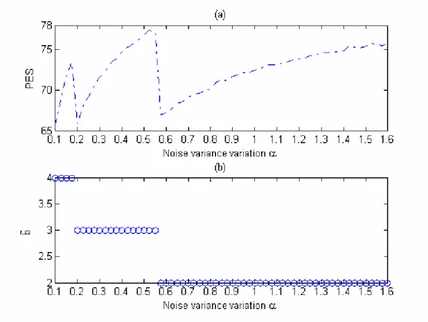
The Figure 3.1(a) shows the PES for 0.1≤ ≤α 1.6 and Figure 3.1(b) depicts the uted b in

comp (3.31) with fixed δ =0.8. That the PES exhibits two “jumps” can be rved. This accounts for the two level change of b as

obse α varies. Within each

tion of constant b , energy efficiency of the optimal solution α

dura improves as

increases (a large α corresponds to a more inhomogeneous sensing environ ent). ilar phenomenon has been observed in the existing works relying dge [6, 7]. When the sensing condition

m We note that a sim

on instantaneous noise variance knowle

effic oise variance description would reflect the long-term characteristic of the schemes [6, 7], this consistency is expected.

iency. Since the proposed solution (3.25) based on statistical n

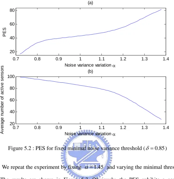
Figure 3.1 : PES for fixed minimal noise variance threshold (δ =0.8)

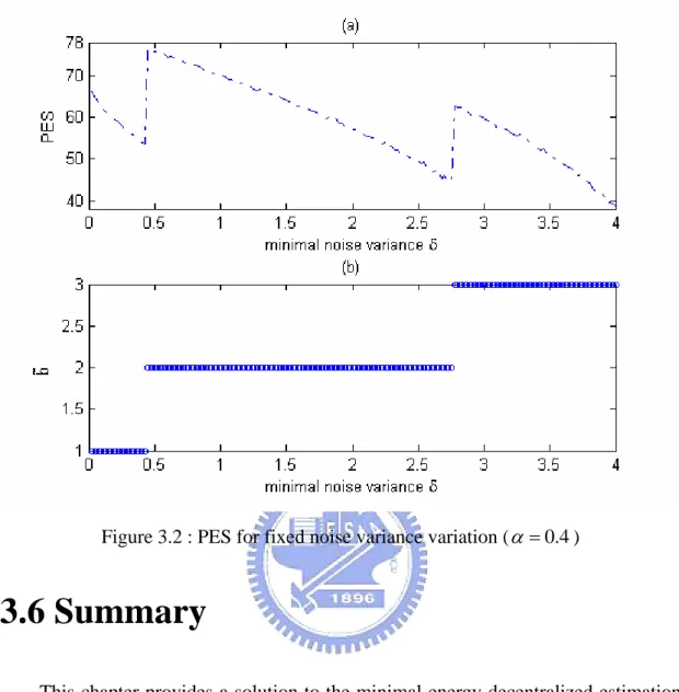
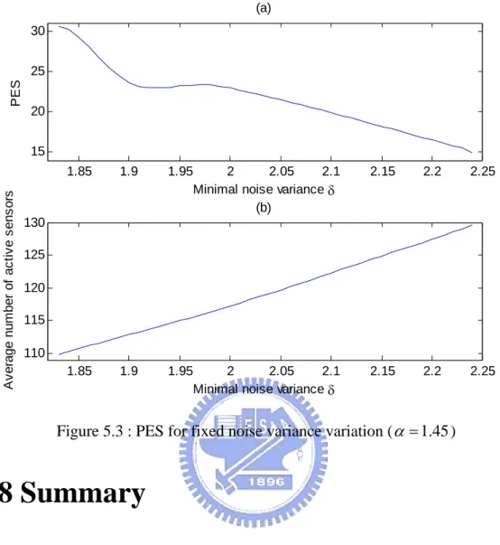
We repeat the experiment by fixing α=0.4 and varying the minimal threshold δ . The results are shown in Figure 3.2. Obviously, the PES exhibits a counter

denc pared t re 3.1. For e ation o

ten y as com o Figu ach dur f constant b , the energy saving achieved by proposed optimal solution is lower as δ increases. This is reasonable because the large minimal noise variance threshold results in severe noise

corru ore sensor n

uf mation

ption in all sensor measurement. M odes should be turned on to provide a s ficient amount of infor for MSE reduction.

Figure 3.2 : PES for fixed noise variance variation (α=0.4)

3.6 Summary

This chapter provides a solution to the minimal-energy decentralized estimation problem by exploiting a statistical noise variance model. Based on a closed-form expression of the MSE performance measure averaged over the noise variance distribution, energy minimization is reformulated as convex optimization problem. The proposed solution simply allocates energies to sensors with large channel gain

nd shut off those suffering from poor link quality. Numerical simulation shows that f reduc

w a

the proposed optimal solution is capable o ing about 80% energy consumption hen compared with the uniform-allocation scheme. The energy saving efficiency is particularly significant when the minimal measurement noise variance threshold is small or the variation factor is large.

Chapter 4

Equation Chapter (Next) Section 1

Minimal Mean Square Error

Decentralized Estimation Based on

Sensor Noise Variance Statistics

Relying on partial noise variance knowledge in the form of the background distribution, the problem of minimizing total transmission energy under an allowable average distortion level is recently considered in [15]. This chapter considers the

o find the optimal bit load which minimizes the average distortion under a fixed total energy budget. The main contribution of the current work

counterpart problem: how t

can be summarized as follows:

i. While the design metric, the reciprocal of the average MSE is shown in [15] to be highly nonlinear in the sensor bit load. Several analytic approximation relations are used to derive an associated tractable low bound.

ii. By maximizing this lower bound, the problem can be further formulated in the form of convex optimization which yields a closed-form solution.

link quality should be shut off toward utmost estimation accuracy, and energy allocated to those active nodes should be proportional to the individual channel gain. A similar energy conservation policy is also found in the previous work [6, 7, 15]. Numerical simulations show the effectiveness of the proposed scheme which outperforms the uniform allocation strategy under an energy-limited environment.

4.1 Average Mean Square Error of

Decentralized Estimation

The MMSE decentralized estimation which is counterpart problem of (3.1) can be formulated as 1 2 1 1 1 Min , subject to , 4 i N N i T b i _i i E E σ β − − = = ⎛ ⎞ ≤ ⎜ ⎟ ⎜ ₊ ⎟ ⎝

∑

⎠

∑

(4.1) or equivalently, 2 1 1 1 Max , subject to , 4 i N N i T b i i i E E σ β − = = ≤ +

∑

∑

(4.2)

where β =R2 12 and is allowable energy level. The equivalent MSE cost function is averaged with respect to the noise variance statistic characterized in (2.2):

T E

( )

1 1 1 Max , subject , 4 i N N i T b i _i i to p d E z δ α β − = = ≤ + +

∑

∑

∫

z z z E (4.3)

where z=

[

z z₁, ₂,....,z_N

]

Τ with p

( )

z denoting the associated distribution. In order

to solve problem (4.3), the first step is to find an analytic expression of the equivalent average MSE metric.

(

)

₍

₎

(

)

4 2 1 Q 4 , subject to . bi i b N N i T i e E E δ β α δ β α − + ₋ = ⎛ ⎞ ⋅ _⎜ + _⎟ ⎝ ⎠ ≤

∑

(4.4)

Exact solution to the considered optimization (4.4) appears formidable to tackle ormulation which is more tractable is proposed and an analytic solution can be obtained. By the

1 Max 2 4 bi i π α δ β − = ⋅ +

∑

because the cost function is highly nonlinear in b . An alternative f_i

following approximation to Q(.) function [16, p115]

( )

(

)

2 2 x 1 1 2 1 Q , 2 _{1 2} e x x x π _π− _π− _π ⎡ ₋ ⎤ ⎢ ⎥ ≈ _{⎢ ⎥} − + + ⎢ ⎥ ⎣ ⎦ (4.5)

and some straightforward manipulations, the cost function can be approximated by

(

)

₍

₎

(

)

(

)

(

)

(

)

(

)

4 2 1 Q 4 2 4 . bi i i b N b i eδ β α δ β α π α δ β − + ₋ − = ⎛ ⎞ ⋅ _⎜ + _⎟ ⎝ ⎠ ⋅ + ≈

∑

∑

(4.6)

The main advantage of (4.6) is that it can lead to an associated lower bound in a more tractable form. Thought maximizing this lower bound we can eventually obtain a closed-form optimal solution. By the inequality equation:

2 1 1 1 1 1 4 i 4 i 2 4 i N i= _−π− _{δ β+} −b _+π− _{δ β+} −b _{+ πα δ β+} −b

(

)

2

(

) (

)

4 bi 2 4 bi 4 bi , δ β+ + πα δ β+ ≤ δ β+ +πα (4.7) ximated cost function in (4.6) can be lower bounded by

− − −

(

)

(

)

(

)

(

)

(

)

(

)

(

)

(

)

2 1 1 1 1 4 4 1 i i b b i π δ β π δ β πα 1 1 1 1 1 1 4 4 2 4 1 4 i i i i N i b b b N N b i π δ β π δ β πα δ β δ β α = − − − − − − − − − = − + + ⎡ + + ⎤ − = − + + + + + ≥ ⎣ ⎦ = + +

∑

∑

∑

(

)

1 4 . 4 i i b N b i= β α δ = + +

∑

We will thus focus on maximizing the lower bound

(4.8) :

(

)

1 1 Max , subject to . 4bi i T i i 4bi N N E E β α δ = = ≤ + +

∑

∑

(4.9)

The cost function is simple in (4.9). It can lead to an analytic solution of the ptimization problem.

gy Density Factor of Sensor Nodes

We assume that each sensor sends messages to FC using a separate channel. This achieved by a m

density N0/2:

o

4.2 Ener

can be using ultiple access technique such as TDMA or FDMA. Each channel is corrupted by additive white Gaussian noise (AWGN) with power spectral

2

ˆ_{i i i} ,

m =d−κ m +v_i (4.10)

is the received

where m ˆ_i message at FC and vi is the AWGN. The signal power

received at the FC is assumed to be inversely proportional to d_iκ where d is the _i

distance between sensor i and the FC, and κ is the path loss exponent common to all sensor-to-FC links.

amplitude modulation with a constellation size 2bi. The consumed energy is [4, 5, 6, 17]

(

2bi 1 , 1

)

i i

E =w − ≤ ≤i N. (4.11)

The energy density factor wi is defined as

2 P κ ⎛ ⎞ ⎝ ⎠ in which ln , i i b w =ρd ⋅ ⎜ ⎟ (4.12)

ρ is a constant depending on the noise profile, and Pb is the target bit error

rate assumed common to all sensor-to-FC links.

With (4.11), the specification of the energy allocated to the ith sensor amounts to etermining the number of quantization bits bi.For a fixed s

d et of noise variances

2

i

σ ’s, the MSE minimization problem subject to an allowable energy level E_T can be formulated as

(

)

(

)

1 1 4 Max , subject to 2 1 . 4 i i i b N N b i T b i i w E β α δ = = − ≤ + +

∑

∑

(4.13) , it follows Since 0b_i ≥

(

)

(

)

1 1 2i 1 4i 1 N N b b i i i i w w = = − ≤ −

∑

∑

. This implies that we can

replace the total energy constraint in (4.13) by the following one without violating the over

=

With the aid of (4.14) and by performing a change of variable with the optimization problem then becomes

all energy budget requirement:

(

)

1 4 i 1 . N b i T w − ≤E

∑

(4.14) i 4bi 1 i B = − ,

(

) (

)

1 1 1 Max , subject to . N N i i i T i i i B w B E B α β δ α δ = = + _≤ + + + +

∑

∑

(4.15)

In (4.15), the intermediate variable B _i

Wh

is relaxed to be a nonnegative real number so as to render the problem tractable. ile the optimal real-valued B is computed, _i

the associated bit loads can be obtain through upper integer rounding. The major advantage of the alternative problem formulation is that it admits the form of convex

ptimization and can lead to a simple closed-form solution. It is shown section.

4.3 Problem Formulation and Optimal

Closed-form Solution

The finial optimization problem is as followed

o in the next

(

) (

)

1 1 1 Max , subject to , 0, 1 . N i i T i w B ≤E B ≥ ≤ ≤i N

∑

(4.16) N i i i i B B α β δ α δ = = + + + + +

∑

In order to solve problem (4.16), let us form the Lagrangian as

(

)

(

) (

)

1,..., N, , 1,..., N L b b λ μ μ 1 1 1 i i T i i i= α β δ+ + + α δ+ Bi ⎝i= ⎠ i=

The associated set of KKT conditions [14] is as followed:

1 . N N N i B w B E B λ⎛ ⎞ μ + =

_∑

− _⎜

_∑

− _⎟+

_∑

(4.17)

(

) (

)

2 i i 0, 1 , i w i B β _{λ μ} N α β δ+ + + α δ+ − + = ≤ ≤ (4.18) ⎡ ⎤ ⎣ ⎦ N i i T i w B E λ = ⎛ ⎞ , 1 0 − = ⎜ ⎟ ⎝

∑

⎠ (4.19) i i i 0, 0, b_i 0, b 0, 1 i N. λ≥ μ ≥ μ = ≥ ≤ ≤ (4.20)

The condition (4.18) leads to 1 1 . i B β β i i w δ λ μ α δ ⎛ ⎞ α = − + − ⎝⎜ + + ⎠⎟ (4.21) λ= μ > ≤ ≤

0, 1 i N

i

b = ≤ ≤ . This case should be precluded since all sensors are turned off. From

(4.19) and (4.21), λ can be obtained:

1 N 1 i α δ 1 ₁ . N i T i i w E w β β λ α δ − = + _{⎝ ⎠⎝} + ₌ ⎛ ⎞⎛ ⎛ = _{⎜ ⎟⎜} + +_{⎜ ⎟ ⎟} ⎝ ⎠ _⎠

∑

∑

(4.22) In (4.21) ⎞ ⎞

,λ and μ_i’s should be determined to fulfill the desired constraints.

1 2 N

w ≥w ≥ ⋅⋅⋅⋅⋅⋅ ≥w is assumed without loss of generality and we define the function

( )

1 1 T i E , 1 . i K N i K N K i w f K = K N = = ≤ ≤ (4.23) 1 β − ⎛ ⎞ w w α δ + + + ⎝ ⎠

∑

Let be the unique integer such that

⎜ ⎟

∑

1≤K ≤N f K

(

₁− < and 1

)

1 . If , then set

( )

1 f K ≥

( )

1

f K ≥ for all 1 K N≤ ≤ K₁= . The existence and uniqueness of such 1

K1 is shown in Lemma 4.1 with proof given in Appendix D.

Lemma 4.1 : f K defined

( )

in (4.23) is monotone increasing and f N

(

)

> . 1 If K1 such that f K

( )

1 ≥ exists, then K1 1+1 will lead to f K

(

1+ ≥ . 1

)

1

The optimal solution pair

(

B_iopt,λopt

)

is given by

1 1 0, 1 -1, 1 opt opt i B w β β α δ λ ⎪ =_{⎨ ⎛ ⎞} + ⎩ ) 1 , , i i K K i N α δ ≤ ≤ ⎧ − +_{⎜ ⎟} ≤ ≤ ⎪ _{⎝ + ⎠} (4.24 where 1 1 i K i K α δ α δ 1 1 . N N opt i T i w E w β β λ − = = + + ⎛ ⎞⎛ _{⎛ ⎞} ⎞ = ⎜_⎜ ⎟⎜_⎟⎜ + +_{⎜ ⎟} ⎟_⎟ ⎝ ⎠ ⎝

∑

⎠⎝

∑

⎠ (4.25) Since 4 i 1 i

1 1 1 2 1 0, 1 1, 1 log 1 , K . opt _{N N} i i j T j i K b w w E β w β i N ≤ ≤ − ⎧ 1 2 _{j K} α δ _{j K} α δ − = = ⎧_{⎡ ⎤ ⎡ ⎤} ⎫ = ⎨ ⎪ _{+ +}⎛ ⎞ ₋ ⎪ _{≤ ≤} ⎢ ⎥ ⎢ ⎥ ⎨ _{+ +} ⎬ ⎝ ⎠ ⎢ ⎥ ⎢ ⎥ ⎪⎣ ⎦ ⎣ ⎜ ⎟ ⎦ ⎪ ⎩ ⎭ ⎪ (4.26)

t average distortion level then equals

∑

∑

⎪ ⎪ ⎪⎩ The resultan

(

)

(

)

1 1 4 2 4 2 opt bi opt i b i K e Q MSE δ β α δ β α π − − ⎛ ⎞ + ⎜ ⎟ ⎜ ⎟ ₋ ⎝ ⎠ = ⎛ ⎞ ⎛ ⎞ ⎜ . 4 iopt N b α δ β − ⎟ + ⎜ ⎟ ⎜ ⎟ ⎝ _{⎠ ⎟} ⎟ + _⎟ ⎜ ⎟ ⎝ ⎠ (4.27)

4.4 Discussions of Optimal Solution

1. The minimal average MSE is attained when all the raw sensor measurements ⎜

= ⋅

⎜ ⎜

∑

with infinite-precision (i.e., b_i =0, 1≤ ≤i N ) are available to the FC. Hence, by setting in the mean MSE formula specified (4.4), we have the following performance bound i b = ∞

(

)

1 2 min 2 Q . MSE Neδ α δ α π − ⎡ αδ ⎤ = ⎢ ⎥ ⎣ ⎦ (4.28)

Formula (4.28) reveals the impacts of the noise model parameters α and δ on the estimation performance. It is easy to see from (4.28) that minim MSE increases with

the al α. This implies the estimation accuracy degrades as the sensing environm es more and more inhomogeneous (corresponding to large

ent becom

α). Furthermore it can be checked that MSEmin also increases with the δ . This is reasonable since large δ

minimal noise power threshold implies

poor measurement quality of all sensor data and a less accurate p rameter estimate. Although these facts are inferred based on

a

with 2. The energy

links with the same ). Large value of wi correspond to sensors deployed far

away from the FC, usually with poor background channel gains. In this point, the proposed optimal solution is intuitively attractive. The senso

the (K1-1)th largest wi’s are turned off to conserve energy. A similar energy

is also found in [6, 7, 15].

s is inversely proportional to sensor data quantization.

density factor wi is proportional to the path loss d (assuming all _iκ

κ

rs associated with

conservation strategy via shutting off sensors with poor channel links

From (4.26), the assigned message length for those active node w . This is intuitively reasonable since _i

sensors with better link conditions should be allocated with more bits (energy) to improve the estimation accuracy.

3. In order to prevent sensors from exhausting energy quickly, one natural way is to impose an additional peak energy constraint:

(

2bi 1

)

, 1 .

i P

w − ≤E i N

requirement (4.29), there does not seem to exist a closed-form optimal solution. As a simple suboptimal

de inde set

≤ ≤ (4.29)

In optimization problem (4.16), with extra inequality

alternative, we can first identify the infeasible no x

(

{

i wi

)

EP, K1 i N

}

Γ = 2biopt − >1 ≤ ≤ from (4.26) _{and then instead fix the}

energy associated with each of these nodes to be EP. The resultant solution is

thus

(

)

1 1 1 2 1 2 0, 1 K 1, 1 log 1 , K and , 2 g 1 , i N N i i j T i j K j K P i i b w w E w i N i E w β β α δ α δ − = = ≤ ≤ − ⎧_{⎡ ⎤ ⎡ ⎤} ⎫ ⎪ ⎛ ⎞ ⎪ = ⎨⎢ ⎥ ⎢ + +⎜ ₊ ⎟ ⎥− ₊ ⎬ ≤ ≤ ∉Γ ⎝ ⎠ ⎢ ⎥ ⎢ ⎥ ⎪⎣ ⎦ ⎣ ⎦ ⎪ ⎩ ⎭ +

∑

∑

1 K i N and i . ⎧ ⎪ ⎪⎪ ⎨ ⎪ ≤ ≤ ∈Γ lo ⎪ ⎪⎩

(4.30) The actual solution can be obtained by using the iterative proced

[18] with (4.30) as an initialization point. The algorithm to derive the optimal analytical solution is followed.

(1) Solve the problem without individual power constraints (4.16) to obtain the solution (4.26).

ures reported in

Set the index set

{

(

2 1

)

, ₁

}

opt i b i P i w E K i N Γ = − > ≤ ≤ .

(

)

2 log 1 opt P i i b = +E (2) Set w for i∈ Γ. Set

(

2bi 1

)

T T i i E =E −

∑

_∈Γw −

ove b for _i i∈ Γ from .

Rem the design variable space.

(3) Repeat the first and second steps until Γ is empty in the first step.

To prove that the algorithm leads to the global optimum, we need only to prove when we that in the second step we do not lose optimality of b_iopt for i∈ Γ

set b_iopt =log₂

(

1+E_P w_i

)

for i∈ Γ.

We compare the sim

4.5 Numerical Simulation

ulated performance of proposed optimal solution (4.26) against the uniform energy allocation scheme with bit load determined through

(

2bi 1

)

, 1

i T

w − =E N ≤ ≤i N. (4.31)

In (4.31), bi is computed via lower integer rounding so that the resultant total energy can be kept below ET. It leads to

2 log T 1 . i b Nw E ⎛ ⎞ = _⎜ + _⎟ ⎝ ⎠ (4.32)

In each independent run we simply choose w_i =d_iκ , where κ =2 and 0.5 0.3

i i

d = + Z with Z_i ∼χ₁2

( )

z being i.i.d.. The total numbe

the following experiments we set the numb N=200, and consider

three . r of trial is 50000. In er of sensors to be 1 N T i i E γ w = =

_∑

with γ =0.25, 1, 3 respectively different levels of total energy

correspond to the low, medium, and high energy cases.

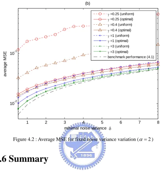
With fixed δ = , Figure 4.1 shows the computed average MSE as 2 α varies 0.5 to 8. With fixed 2

from α= , Figure 4.2 shows the average MSE as δ varies 0.5 to 8. Both figures show that the estimation accuracy improves as E from

increases. It is expect alloc

environm

T

ed. The proposed solution (4.26) outperforms uniform energy ation (4.32), especially when ET is small. It is more effective in an energy-limited

ent. The simulated average MSE increases with both α and β .

100

0 1 2 3 4 5 6 7 8

10-2 10-1

noise variance variation α

av e rag e M S E (a) γ =0.25 (uniform) γ =0.25 (optimal) γ =0.4 (uniform) γ =0.4 (optimal) γ =1 (uniform) γ =1 (optimal) γ =3 (uniform) γ =3 (optimal) benchmark performance (4.1) 2 δ = Figure 4.1 : Average MSE for fixed minimal noise variance threshold ( )

1 2 3 4 5 6 7 8 10-2 10-1 minim se va nce δ a v er age M S E (b) γ =0.25 (uniform) γ =0.25 (optimal) γ =0.4 (uniform) γ =0.4 (optimal) γ =1 (uniform) γ =1 (optimal) γ =3 (uniform) γ =3 (optimal) benchmark performance (4.1) al noi ria

Figure 4.2 : Average MSE for fixed noise variance variation (α = ) 2

4.6 Su

This chapter provides a solution to th ma ation problem

expre

distribution, MSE minimization is reformulated as convex optimization problem. The analytic closed-form solution reveals the energy saving policy. The proposed solution channel gain and shut off those suffering from poor link quality. Numerical simulation shows that the estimation accu

hus is ore effective in an energy-limited environment.

mmary

e mini l-MSE decentralized estim by exploiting a statistical noise variance model. Based on a closed-form ssion of the MSE performance measure averaged over the noise variance

simply allocates energies to sensors with a large

racy improves as total energy increases. The proposed solution outperforms uniform energy allocation especially when the total used energy is small, and t

Chapter 5

Equation Chapter (Next) Section 1

Minimal Energy Decentralized

r Noise

n esign, the minimal-energy decentralized estimation problem which is formulated in an optimal bit-loading setup has been recently considered. In order to improve the estimation performance against the variation of sensing conditions, repeated update of the noise profile would be needed. This comes inevitably at the cost of more training overhead and extra energy consumption. One typical approach to resolving such a drawback is to exploit the partial (or long-term) information of the noise characteristics.

Another key feature common to the existing related works [1, 6, 7 ] is that they all assume error-free transmission. They consider the sensors experiencing the perfect wireless channel. There is no bit error in the wireless channels between sensors and

Estimation over Rayleigh Fading

Channel Based on Senso

Variance Statistics

the FC. The work in [6] uses the upper bound (2.15) to show that the actual achieved MSE is at most a constant factor away from what is achievable with perfect sensor channels. It use the MSE constraint with perfect channel to formulate the convex optimization problem which derive an optimal bit loading scheme. Chapter 3 and Chapter 4 of my thesis also use the MSE constraint with perfect channel to formulate the optimization problems instead by the long-term information of the noise characteristics. The work in [19] considers the noisy channel between each sensor and the FC by modeling it as a binary symmetric channel (BSC) model with crossover probability which is controlled by the transmitted bit energy, but it uses the instantaneous local sensor noise characteristics to formulate the optimization problem.

This chapter attempts to provide a solution to the minimal-energy decentralized estimation with the noisy channel between each sensor and the FC by exploiting long

term ] for ise

variance is used and the estimation performance is assessed through an MSE based metric average with respect to the considered distribution. The BSC models [19] are used to characterize the wireless multi-path fading channels with path loss. A closed-form expression for the overall MSE requirement is derived. The analysis of the energy-minimization problem is formulated in the form of convex optimization. The problem is then analytically solved.

The proposed suboptimal scheme shares several interesting aspects pertaining to those based on the instantaneous noise variance information. Sensors with bad channel quality (specified via the path distance to FC) are shut off to conserve energy, and for those active nodes the allocated energy is proportional to the individual channel gain. Simulation results show that the proposed optimal solution yields energy saving against the equal-bit allocation policy.

5.1 System Model

There are N spatially deployed sensors which cooperate with a FC for estimating an unknown deterministic parameter θ where θ∈

[ ]

0, 1 . In order to simplify the

[ ]

following analysis, we set θ∈ 0, 1 which is a special case for general case

[

R 2, 2R

]

θ∈ − where R is the parameter range. The following analytic results for

the general case and special case are different in a constant factor. The local observation at the ith node is

, x_i = +θ n_i 1≤ ≤i N, (5.1)

where ni is a zero-mean measurement noise with variance [6, 7]

2

.

i zi

σ = +δ α (5.2)

In (5.2), δ models the network-wide noise variance threshold, α controls the underlying variation from the nominal minimum, and z_i ∼χ₁2 is a central Chi-Square distributed random variable with degrees-of-freedom equal to one. Due to bandwidth and power limitations each sensor quantizes its observation into a bi-bit

message, and then transmits this locally processed data to the FC to generate a final estimate of θ.

The uniform quantization scheme with nearest-rounding is adopted. The quantized message at the ith sensor can be modeled as

, m_i = +x_i q_i 1≤ ≤i N, (5.3)

where qi is the quantization error which is uniformly distributed with zero mean and

variance 2 1 12 4

(

i

)

i

b q

σ = ⋅ , and [0, 1] is the available signal amplitude range common