利用隨機邊界法估計台灣各縣市之總要素能源效率

行政院國家科學委員會專題研究計畫 成果報告

利用隨機邊界法估計台灣各縣市之總要素能源效率

研究成果報告(精簡版)

中 華 民 國 101 年 10 月 30 日

中 文 摘 要 ： 自 Hu and Wang (2006) 及 Hu and Kao (2007) 首次提出總 要素能源效率（TFEE）指標以來，後續應用 TFEE 指標的實證 研究一直利用資料包絡分析法（DEA）來進行能源投入目標值 （或總能源投入差額）的計算。在引述 Hu and Wang (2006) 下，Zhou et al. (2012) 利用將單一方程式、隨機邊界生產 函數移項的方式，推導出總要素能源效率的估計式。然而 Zhou et al. (2012) 的版本目前仍只考慮橫斷面（cross section），並只利用 2001 年 21 個 OECD 國家的資料作分 析。本計畫進一步將之延伸改寫為縱橫面資料（panel）型 式，並將用以估計台灣 23 縣市在 2004-2008 年期間的總要素 能源效率。 本計畫自行延伸並推導的隨機邊界法模型，符合 Battese and Coelli (1992) 的縱橫面資料、隨機邊界法模型之設 定，並可利用 Coelli 教授所提供的免費軟體 Frontier 4.1 進行估計。模型中有一項產出項：各縣市所得，及六項投入 項：各縣市就業人口、生產用電力用電量、家庭電燈用電 量、其他非家庭電燈用電量、汽油用油量、柴油用油量等。 名目變數藉由 GDP 平減指數轉換為以 2005 為基期的實質變 數。實證結果與 Hu et al. (2012) 利用資料包絡分析法的 發現大致上一致：隨機邊界法所得到的總要素能源效率排序 非常穩定。大多數台灣各縣市在各項能源使用上皆呈現無效 率狀態。在 2004 年至 2008 之間台灣各縣市平均的總要素能 源效率值為：生產用電力用電 (0.6444)、家庭電燈用電 (0.875134)、非家庭其他電燈用電 (0.895671)、汽油 (0.846243)、柴油 (0.672207)。可知台灣各縣市的生產用電 力及柴油使用效率特別需要提升。有製造業聚落的科學園區 或工業區的縣市宜優先提升生產用電力的效率。非都會區縣 市宜優先提升家庭電燈用電效率及非家庭其他電燈用電效 率。台灣各縣市皆須改善汽油使用效率。非都會縣市宜優先 提升柴油使用效率。 中文關鍵詞： 隨機邊界法、總要素能源效率、縱橫面資料

英 文 摘 要 ： This research applies the panel data stochastic production frontier to estimate total factor-energy efficiency (TFEE) scores for regions in Taiwan during 2004-2008. The panel data stochastic frontier

analysis (SFA) model to estimate TFEE is extended from the cross-section version of Zhou et al. (2012). This SFA panel data model can be empirically

estimated by using that proposed by Battese and Coelli (1992) and hence the free software kindly

provided by Professor T.J. Coelli (1996) can be used for estimation. This paper is an effort to

complement the work of the TFEE index proposed by Hu and Wang (2006)； moreover, it is also a very good experiment to further try to extend the SFA modeling for estimating energy efficiency.

There are six inputs (the employed population, amount of productive electricity power consumed, amount of electricity consumed for household electric light, amount of electricity consumed for non-household electric light, amount of gasoline sales, and amount of diesel sales) and one output (the total real income in the base year of 2005) in the SFA models. Note that the rankings in TFEE scores of the same energy source, obtained by the SFA models, are all stable over time. Most administrative regions in Taiwan are not efficient in almost all kinds of energy use. The average TFEE scores in various energy sources during 2004-2008 are: productive electricity power (0.6444), household lighting (0.875134), non-household lighting (0.895671), gasoline (0.846243), and diesel (0.672207). It can be seen that the efficiencies of using productive electricity power and diesel need to improve very much. It is a priority for regions where

manufacturing and high-tech industries concentrate to achieve more efficient use of productive electricity. It is a priority for non-metropolitan regions to

improve the efficiency of both household and non-household lighting. It is a priority for all regions to improve the motor-vehicle energy efficiency in order to improve gasoline efficiency. It is a

priority for non-metropolitan regions to improve the diesel use efficiency.

英文關鍵詞： Stochastic Frontier Analysis (SFA), Total-factor Energy Efficiency (TFEE), Panel Data

利用隨機邊界法估計台灣各縣市之總要素能源效率

Applying the Stochastic Frontier Analysis to Estimate the

Total-Factor Energy Efficiency for Regions in Taiwan

計畫編號：NSC 100-2410-H-009 -051

計畫報告

執行期限：民國 100 年 8 月 1 日至 101 年 7 月 31 日

主持人：胡均立 國立交通大學經營管理研究所

兼任研究助理：潘京蒂、李昱墨、盧煒婷、張嘉文、簡瑞祥

電子信箱(E-mail)位址：

jinlihu@mail.nctu.edu.tw

關鍵字：隨機邊界法、總要素能源效率、縱橫面資料

中文摘要

自 Hu and Wang (2006) 及 Hu and Kao (2007) 首次提出總要素能

源效率（TFEE）指標以來，後續應用 TFEE 指標的實證研究一直利

用資料包絡分析法（DEA）來進行能源投入目標值（或總能源投入

差額）的計算。在引述 Hu and Wang (2006) 下，Zhou et al. (2012) 利

用將單一方程式、隨機邊界生產函數移項的方式，推導出總要素能

2

源效率的估計式。然而 Zhou et al. (2012) 的版本目前仍只考慮橫斷

面（cross section），並只利用 2001 年 21 個 OECD 國家的資料作分

析。本計畫進一步將之延伸改寫為縱橫面資料（panel）型式，並用

以估計台灣 23 縣市在 2004-2008 年期間的總要素能源效率。

本計畫自行延伸並推導的隨機邊界法模型，符合 Battese and

Coelli (1992) 的縱橫面資料、隨機邊界法模型之設定，並可利用

Coelli 教授所提供的免費軟體 Frontier 4.1 進行估計。模型中有一項

產出項：各縣市所得，及六項投入項：各縣市就業人口、生產用電

力用電量、家庭電燈用電量、其他非家庭電燈用電量、汽油用油

量、柴油用油量等。名目變數藉由 GDP 平減指數轉換為以 2005 為

基期的實質變數。實證結果與 Hu et al. (2012) 利用資料包絡分析法

的發現大致上一致：隨機邊界法所得到的總要素能源效率排序非常

穩定。大多數台灣各縣市在各項能源使用上皆呈現無效率狀態。在

2004 年至 2008 之間台灣各縣市平均的總要素能源效率值為：生產用

電力用電 (0.6444)、家庭電燈用電 (0.875134)、非家庭其他電燈用電

(0.895671)、汽油 (0.846243)、柴油 (0.672207)。可知台灣各縣市的

生產用電及柴油使用效率特別需要提升。有製造業聚落的科學園區

或工業區的縣市宜優先提升生產用電力的效率。非都會區縣市宜優

3

先提升家庭電燈用電效率及非家庭其他電燈用電效率。台灣各縣市

皆須改善汽油使用效率。非都會縣市宜優先提升柴油使用效率。

4

二、英文摘要及全文初稿

The Total-factor Energy Efficiency of Regions in Taiwan:

An Application of the Stochastic Frontier Analysis

Jin-Li Hu

Institute of Business Management, National Chiao Tung University

Taiwan

Abstract

This research applies the panel data stochastic production frontier to estimate total factor-energy efficiency (TFEE) scores for 23 administrative regions in Taiwan during 2004-2008. The panel data stochastic frontier analysis (SFA) model to estimate TFEE is extended from the cross-section version of Zhou et al. (2012). This SFA panel data model can be empirically estimated by using that proposed by Battese and Coelli (1992) and hence the free software kindly provided by Professor T.J. Coelli (1996) can be used for estimation. This paper is an effort to complement the work of the TFEE index proposed by Hu and Wang (2006); moreover, it is also a very good experiment to further try to extend the SFA modeling for estimating energy efficiency.

There are six inputs (the employed population, amount of productive electricity power consumed, amount of electricity consumed for household electric light, amount of electricity consumed for non-household electric light, amount of gasoline sales, and amount of diesel sales) and one output (the total real income in the base year of 2005)

5

in the SFA models. Note that the rankings in TFEE scores of the same energy source, obtained by the SFA models, are all stable over time. Most administrative regions in Taiwan are not efficient in almost all kinds of energy use. The average TFEE scores in various energy sources during 2004-2008 are: productive electricity power (0.6444), household lighting (0.875134), non-household lighting (0.895671), gasoline (0.846243), and diesel (0.672207). It can be seen that the efficiencies of using productive electricity power and diesel are needed to improve very much. It is a priority for administrative regions where manufacturing and high-tech industries to concentrate to achieve more efficient use of productive electricity. It is a priority for metropolitan regions to improve the efficiency of both household and non-household lighting. It is a priority for all administrative regions to improve the motor-vehicle energy efficiency in order to improve gasoline efficiency. It is a priority for non-metropolitan regions to improve the diesel use efficiency.

Keywords: Stochastic Frontier Analysis (SFA), Total-Factor Energy Efficiency

(TFEE), Panel Data

*

This is a preliminary draft. Mailing address: 118, Chung-Hsiao W. Rd., Sec.1, Taipei City, Taiwan 10044. FAX: +886-2-2344922; Email: jinlihu@mail.nctu.edu.tw; URL: http://jinlihu.tripod.com.

6

Introduction

Taiwan is insufficient in natural resources and constrained by a limited environment-carrying capacity (Ministry of Affairs 2008). Since 97.9% of Taiwan’s total energy consumption is imported (Bureau of Energy 2008), the foreign market fluctuations or policy changes can easily affect its energy supply and security. Because energy has great impacts on economic development as well as ecological environment, whether or not the energy use is efficient is an important issue for Taiwan.

Since Hu and Wang (2006) and Hu and Kao (2007) first proposed the total-factor energy efficiency (TFEE) index, the follow-up empirical papers have been applying the data envelopment (DEA) approach to compute the energy input target (or the total energy input slack). By referring to Hu and Wang (2006), Zhou, Ang and Zhou (2012) derive an econometric equation for estimating TFEE via re-arranging a single-equation stochastic production function. The current version of Zhou, Ang and Zhou (2012) is still for only cross section data and analyzes 21 OECD countries in the year 2001. This paper further extends the cross-section SFA model of Zhou, Ang and Zhou to a panel data, stochastic frontier analysis (SFA) model. The total-factor energy efficiency scores of 23 administrative regions in Taiwan from 1999 to 2008 will be estimated by this extended panel data SFA model. Fortunately, the panel data SFA approach of Battese and Coelli (1992) can be used to estimate by this extended panel data SFA model.

The application of the total-factor energy efficiency index to Taiwan’s regions can be found in Hu et al. (2012). Their study applies data envelopment analysis (DEA) to compute the efficient energy-saving ratios for 23 administrative regions in Taiwan from 1999-2005. One output (total income) and seven inputs (local government expenditure, employment, processed trash, household and commercial

7

electricity consumption, industrial electricity consumption, gasoline sales volume, and diesel sales volume) are considered in the DEA models. It is found that most of the 23 administrative regions do not efficiently use household and commercial electricity, industrial electricity, gasoline, and diesel, even with respect to Taiwan’s own efficiency frontier. Their results suggest that improving energy efficiency in household and commercial electricity use is a priority for non-metropolitan regions. There is still much room to improve the efficiency of electricity use for industries, especially for regions where manufacturing and high-tech industries concentrate, by means of cleaner production, energy-saving technology and equipment, etc. Motor vehicle energy efficiency is the key factor for saving gasoline. The energy efficiency of farming machines and carrying equipment should be continuously improved, especially for rural regions.

Hu et al. (2011) applies the four-stage DEA procedure to calculate the energy efficiency of 23 regions in Taiwan from 1998 to 2007. After controlling for the effects of external environments, only Taipei City, Chiayi City, and Kaohsiung City are energy efficient. Note that Kaohsiung City reaches the efficiency frontier due to the adjustment via partial environmental factors such as higher education attainment and transport vehicles. They also find a worsening trend for Taiwan’s energy efficiency. Not only is there a gap of energy efficiency between Taiwan’s metropolitan and non-metropolitan regions, but the gap has also widened in recent years. Those inefficient counties should be given priority and the savings potential. Except for road density, the evidence indicates that each environmental factor has partial incremental effects on input slacks. As more cars and motorcycles are unfavorable externalities affecting partial energy efficiency, the central government should help local governments retire inefficient old motor vehicles, encourage energy-saving vehicle models, and provide convenient mass transportation systems. Besides, people with higher education cause

8

industrial energy inefficient in Taiwan. The consciousness of effective energy saving is necessary to schools, communities, and employee accordingly.

This paper is a follow-up work which is most similar to Hu et al. (2012) by applying the panel data stochastic production frontier to estimate TFEE scores for 23 administrative regions in Taiwan. Instead of the sample period of 1999-2005, this paper uses the data during 2004-2008. Similar patterns with those found in Hu et al. (2012) are found by the SFA approach extended from Zhou et al. (2012). This paper is an effort to complement the work of the TFEE index proposed by Hu and Wang (2006); moreover, it is also a very good experiment to further try to extend the SFA modeling for estimating energy efficiency.

Research Methodology

Zhou et al. (2012) apply the single-equation, output-oriented stochastic frontier analysis (SFA) model to estimate the total-factor energy efficiency. Their version is still a cross-section SFA model, which analyze 21 OECD countries in 2001. Combining Zhou et al. (2012) and Battese and Coelli (1992), this paper further extends a panel data SFA model to estimate the total-factor energy efficiency.

Following Zhou et al. (2012), we assume that the stochastic frontier distance function is in the Cobb-Douglas functional form:

ln D (Kit, Lit, Eit, Yit) = 0 + k lnKit + L lnLit + E lnEit + E lnYit + vit (1)

where D() is the distance function, Kit is the capital stock, Lit is labor employment, Eit

is the energy input, Yit is the real economic output, i indicates the region, and t indicates the time, and vit is the statistical noise following the normal distribution,.

Since the distance function is homogeneous of degree one in the energy input, the above equation can be re-arranged as:

9 which can be also arranged as

-lnEit = 0 + klnKit + LlnLit + E ln1 + ElnYit + vit - lnDE (Kit, Lit, Eit, Yit)(3)

That is,

ln(1/Eit) = 0 + k lnKit + L lnLit + E lnYit + vit - uit (4)

where uit is the ineffciency term which follows a non-negative distribution and vit -

uit is the error component term of a stochastic production frontier. Eq. fits in the panel data, stochstic frontier model proposed by Battese and Coelli (1992). The free software Frontier 4.1 kindly provided by Professor Coelli (1996) can be used to estimate Eq (4). The total-factor energy effciency of region i at time t then is

TFEEit = exp(-uit) (5)

Therefore, we then can apply the panel data, stochastic production frontier approach to estimate the total-factor energy efficiency and are limited to use the input-oriented data envelopment analysis (DEA) suggested by Hu and Wang (2006) and Hu and Kao (2007). Moreover, if we use disaggregate energy inputs, we can also change the logged inverse energy input on the left-hand side of Eq. (4) and keep other logged inputs on the right-hand side of Eq. (5), such that we can obtain the TFEE scores of different energy inputs.

Data and Variables

The data are regional and annual for 23 administrative regions in Taiwan during 2004-2008. There are six inputs (the employed population, amount of productive electricity power consumed, amount of electricity consumed for household electric light, amount of electricity consumed for non-household electric light, amount of gasoline sales, and amount of diesel sales) and one output (the total real income) in the stochastic frontier analysis (SFA) models.

The data of productive electricity power, electricity of household light, non-household light are from Taiwan Power Company. The productive electricity power usage refers to non-lighting electricity usage including most of the production and service operations. The data of gasoline and diesel sales are from Bureau of Energy, Administrative Yuan. The data of regional income is obtained by multiplying the

10

average household income and the total number of households, from the National Statistics maintained by Directorate-General of Budget, Accounting, and Statistics, Administrative Yuan. The nominal total income is converted into the real income in 2005 prices by dividing the GDP deflator. Therefore, this is a panel data set of 23 administrative regions in Taiwan from 2004 to 2008.

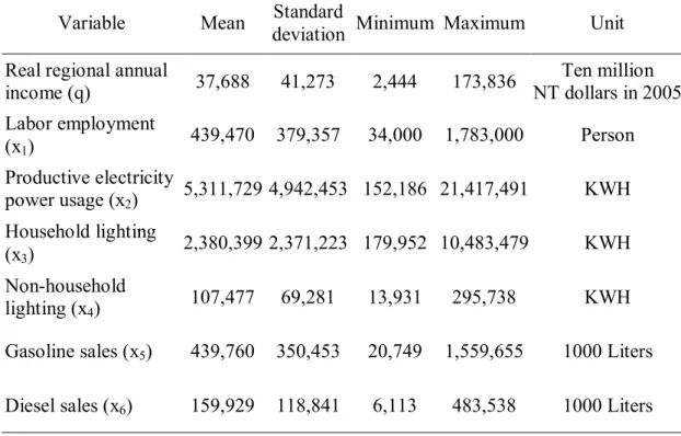
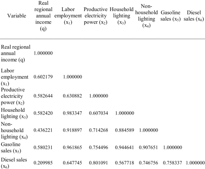
The definitions and units of these input and output variables can be found in Table 1. Table 2 lists the correlation coefficients among these input and output variables. The isotonicity property that an output cannot decrease as an input increases is satisfied.

Empirical findings

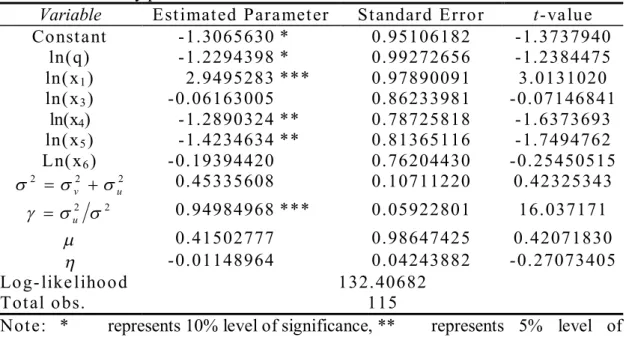
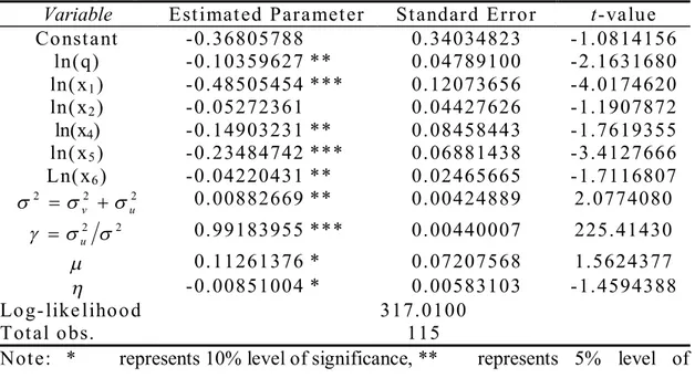
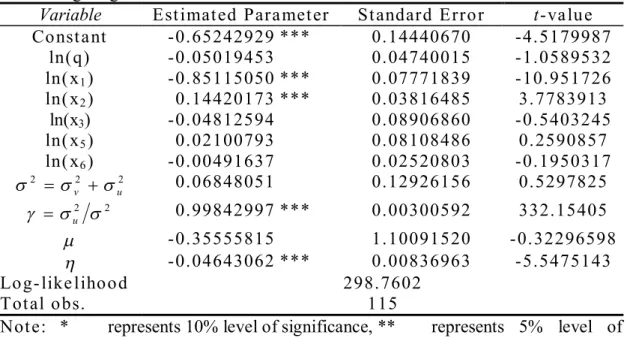
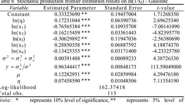
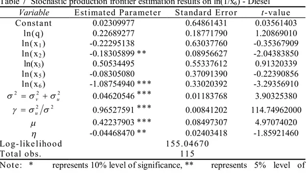
Tables 3-7 list the SFA regression results on each logged inversed energy input. As the methodology section shows, the efficiency score obtained from the SFA model depicted in Eq. (4) is exactly the TFEE score for region i at time t.

The parameter  is the proportion of variance in the inefficiency term (u) to the total variance of the error component term (v - u). As Tables 3-7 show, all estimated  values are significantly different from zero and more than 0.9, indicating that the stochastic frontier analysis model is more appropriate than the ordinary least square method by taking into account the inefficiency term.

As Coelli et al. (2005) define, the parameter  is the parameter for a non-negative

truncated distribution. An estimated  which is not significantly different from zero

implies that the inefficiency term u should follow the half normal distribution. On the contrary, an estimated  which is significantly different from zero implies that the

inefficiency term u should follow a truncated normal distribution. Tables 3-7 show that most of the inefficiency terms should follow truncated normal distributions.

11

The parameter  indicates the trend of time-varying inefficiency. A negative

(positive)  implies that the inefficiency is decreasing (increasing) over time.

Therefore, productive electricity power usage has no significant efficiency changes over time. Household lighting, non-household lighting, and diesel showed decreasing inefficiency (improving TFEE scores). However, the use of gasoline showed increasing inefficiency (worsening TFEE scores).

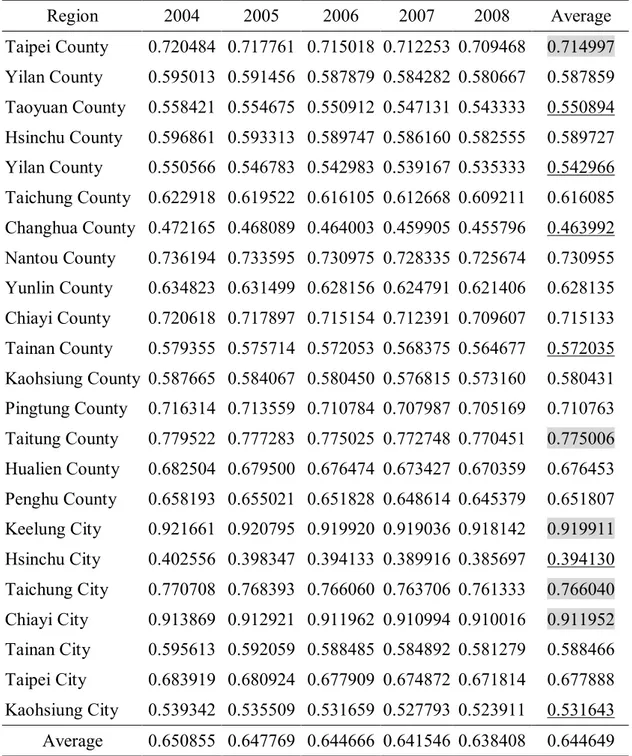
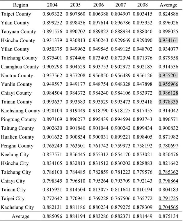
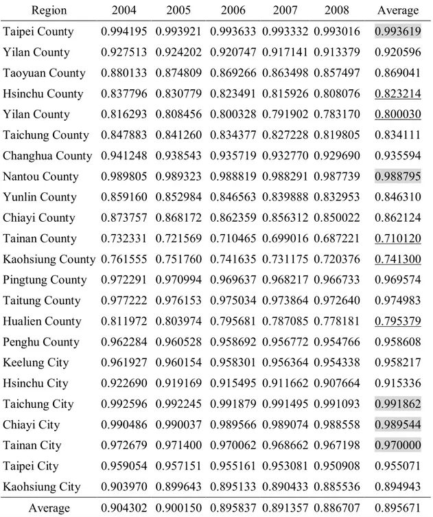
Note that the rankings in TFEE scores of the same energy source, obtained by the SFA models, are all stable over time. Most administrative regions in Taiwan are not efficient in almost all kinds of energy use. The average TFEE scores in various energy sources during 2004-2008 are: productive electricity power (0.6444), household lighting (0.875134), non-household lighting (0.895671), gasoline (0.846243), and diesel (0.672207). It can be seen that the efficiencies of using productive electricity power and diesel are needed to improve very much.

The five most productive electricity power-efficient regions in Taiwan are: Keelung City (0.919911), Chiayi City (0.911952), Taitung County (0.775006), Taichung City (0.766040), and Taipei County (0.714997). The five most productive electricity power-inefficient regions in Taiwan are: Hsinchu City (0.394130), Changhua County (0.463992), Taoyuan County (0.550894), Yilan County (0.542966), and Tainan County (0.572035). Among them Hsinchu City and Tainan County have science parks while Changhua County, Taoyuan County, and Yilan County have large industrial parks. These regions are of many manufacturing industries.

Using the average TFEE scores, the five most household lighting-efficient regions in Taiwan are: Chiayi County (0.986128), Tainan County (0.978335), Yilan County (0.955966), Nantou County (0.955201), and Hsinchu County (0.934161). All of these top five lighting-efficient regions are non-metropolitan areas. Using the average TFEE scores, the five most household lighting-inefficient regions in Taiwan are:

12

Kaohsiung City (0.704565), Penhgu County (0.780697), Taichung City (0.785362), Taipei City (0.791725), and Chiayi City (0.798864). Four out of the five most lighting-inefficient regions in Taiwan are metropolitan regions.

Using the average TFEE scores, the five most non-household lighting-efficient regions in Taiwan are: Taipei County (0.993619), Taichung City (0.991862), Chiayi City (0.9895449), Taitung County (0.974983), and Pingtung County (0.969574). Using the average TFEE scores, the five most non-household lighting-inefficient regions in Taiwan are: Tainan County (0.710120), Kaohsiung County (0.741300), Hualien County (0.795379), Yilan County (0.800030), and Hsinchu County (0.823214). The five most non-household lighting-inefficient regions in Taiwan are all non-metropolitan regions.

Using the average TFEE scores, the five most gasoline-efficient regions in Taiwan are: Penghu County (0.997407), Yilan County (0.908660), Changhua County (0.897513), Kaohsiung City (0.887033), and Hualien County (0.881621). Four out of the five most gasoline-efficient regions in Taiwan are non-metropolitan regions. Using the average TFEE scores, the five most gasoline-inefficient regions in Taiwan are: Taichung City (0.760268), Chiayi City (0.779064), Nantou County (0.798919), Hsinchu County (0.790638), and Tainan County (0.798919). The five most gasoline-inefficient regions in Taiwan are metropolitan as well as non-metropolitan regions.

Using the average TFEE scores, the five most diesel-efficient five regions in Taiwan are: Taipei City (0.976926), Hsinchu City (0.958829), Tainan City (0.879633), Chiayi City (0.778340), and Taichung City (0.768783). All these five most diesel-efficient regions in Taiwan are metropolitan regions. Using the average TFEE scores, the five most diesel-inefficient regions in Taiwan are: Hualien County (0.549941), Yilan County (0.565606), Taichung County (0.574413), Yunlin County

13

(0.575256), and Taitung County (0.592946). The five most diesel-inefficient regions in Taiwan are all non-metropolitan regions.

Conclusion

This paper applies the panel data stochastic production frontier to estimate TFEE scores for regions in Taiwan, using the panel data during 2004-2008. The SFA approach extended from the cross-section SFA of Zhou et al. (2012) to a panel-data SFA. This paper is an effort to complement the work of the TFEE index proposed by Hu and Wang (2006) and Hu and Kao (2007).

Most administrative regions in Taiwan are not efficient in almost all kinds of energy use. The average TFEE scores in various energy sources during 2004-2008 are: productive electricity power (0.6444), household lighting (0.875134), non-household lighting (0.895671), gasoline (0.846243), and diesel (0.672207). That is, the efficiencies of using productive electricity power and diesel need to improve very much.

Although here we use a different sample period and a different methodology, the empirical findings are generally consistent with Hu et al. (2012) who use the DEA approach to compute TFEE scores. Based on the empirical findings, we come up with the following energy efficiency policy suggestions:

1. It is a priority for regions where manufacturing and high-tech industries concentrate to achieve more efficient use of productive electricity. Firms should be encouraged with incentive measures and administrative schemes to engage in cleaner production and adopt energy-conserving technology and equipments. The industrial sector can be restructured towards a high value-added and low energy intensive structure.

14

household and non-household lighting. For these regions, energy-saving facilities such as LED bulbs should be especially encouraged.

3. It is a priority for all regions to improve the motor-vehicle energy efficiency in order to improve gasoline efficiency. Both of the central and local governments should put more efforts on retiring inefficient old motor vehicles, encouraging energy-saving vehicle models, providing convenient mass transportation systems to reduce the usage of private vehicles, and building the user-oriented and green-oriented municipal transportation environment.

4. It is a priority for non-metropolitan regions to improve the diesel use efficiency. Energy efficiency of farming machines and diesel trucks should be continuously improved especially for these regions. The local administrations of these regions should encourage these equipments to change into hybrid energy systems with financial incentives such as tax reductions and subsidies.

References

Battese, G.E. and T.J. Coelli (1992), Frontier Production Functions, Technical Efficiency and Panel Data: With Application to Paddy Farmers in India,

Journal of Productive Analysis, 3, 153-169.

Bureau of Energy 2008. Taiwan Energy Statistical Hand Book. Taipei.

Coelli, T.J. (1996), A Guide to FRONTIER Version 4.1: A Computer Program for Stochastic Frontier Production and Cost Function Estimation, CEPA Working Paper 96/7, University of New England, Armidale, NSW, Australia.

Coelli, T.J., D.S.P. Rao, C.J. O’Donnell and G.E. Battese (2005), An Introduction to

Efficiency and Productivity Analysis, 2nd ed., Springer.

Hu, J.L. and C.H. Kao (2007), Efficient Energy-saving Targets for APEC Economies. Energy Policy, 34, 373–382.

15

Hu, J.L., M.C. Lio, C.H. Kao and Y.L. Lin (2012), Total-factor Energy Efficiency for Regions in Taiwan, Energy Sources, Part B, 7(3), 292-300.

Hu, J.L., M.C. Lio, F.Y. Yeh and C.H. Lin (2011), Environment-adjusted regional energy efficiency in Taiwan, Applied Energy, 88, 2893-2899.

Hu, J.L., and S.C. Wang (2006), Total-factor energy efficiency of regions in China.

Energy Policy, 34, 3206–3217.

Zhou, P., B.W. Ang and D.Q. Zhou (2012), Measuring Economy-wide Energy Efficiency Performance: A Parametric Frontier Approach. Applied Energy, 90, 196-200.

16

Table 1 The summary of statistics of output and input variables Variable Mean Standard

deviation Minimum Maximum Unit Real regional annual

income (q) 37,688 41,273 2,444 173,836 Ten million NT dollars in 2005 Labor employment (x1) 439,470 379,357 34,000 1,783,000 Person Productive electricity power usage (x2) 5,311,729 4,942,453 152,186 21,417,491 KWH Household lighting (x3) 2,380,399 2,371,223 179,952 10,483,479 KWH Non-household lighting (x4) 107,477 69,281 13,931 295,738 KWH

Gasoline sales (x5) 439,760 350,453 20,749 1,559,655 1000 Liters

17

Table 2 Correlation coefficient among the output and input variables

Variable Real regional annual income (q) Labor employment (x1) Productive electricity power (x2) Household lighting (x3) Non-household lighting (x4) Gasoline sales (x5) Diesel sales (x6) Real regional annual income (q) 1.000000 Labor employment (x1) 0.602179 1.000000 Productive electricity power (x2) 0.582644 0.630882 1.000000 Household lighting (x3) 0.582420 0.983347 0.607034 1.000000 Non-household lighting (x4) 0.436221 0.918897 0.714268 0.884589 1.000000 Gasoline sales (x5) 0.580231 0.961865 0.754496 0.944641 0.907651 1.000000 Diesel sales (x6) 0.209985 0.647745 0.801091 0.567718 0.746756 0.758337 1.000000

18

Table 3 Stochastic production frontier estimation results on ln(1/x2) - Productive

electricity power

Variable Est imat ed Para met er St andard Erro r t-va lu e

Co nst a nt -1.3065630 * 0.95106182 -1.3737940 ln(q) -1.2294398 * 0.99272656 -1.2384475 ln( x1) 2.9495283 *** 0.97890091 3.0131020 ln( x3) -0.06163005 0.86233981 -0.07146841 ln(x4) -1.2890324 ** 0.78725818 -1.6373693 ln( x5) -1.4234634 ** 0.81365116 -1.7494762 Ln( x6) -0.19394420 0.76204430 -0.25450515 2 2 2 u v      0.45335608 0.10711220 0.42325343 2 2 _    _u 0.94984968 *** 0.05922801 16.037171  0.41502777 0.98647425 0.42071830  -0.01148964 0.04243882 -0.27073405 Lo g- like liho o d 132.40682 Tot al o bs. 115

Not e: * represents 10% level of significance, ** represents 5% level of significance, *** represents 1% level of significance.

19

Table 4 Stochastic production frontier estimation results on ln(1/x3) - Household

lighting

Variable Est imat ed Para met er St andard Erro r t-va lu e

Co nst a nt -0.36805788 0.34034823 -1.0814156 ln(q) -0.10359627 ** 0.04789100 -2.1631680 ln( x1) -0.48505454 *** 0.12073656 -4.0174620 ln( x2) -0.05272361 0.04427626 -1.1907872 ln(x4) -0.14903231 ** 0.08458443 -1.7619355 ln( x5) -0.23484742 *** 0.06881438 -3.4127666 Ln( x6) -0.04220431 ** 0.02465665 -1.7116807 2 2 2 u v      0.00882669 ** 0.00424889 2.0774080 2 2 _    _u 0.99183955 *** 0.00440007 225.41430  0.11261376 * 0.07207568 1.5624377  -0.00851004 * 0.00583103 -1.4594388 Lo g- like liho o d 317.0100 Tot al o bs. 115

Not e: * represents 10% level of significance, ** represents 5% level of significance, *** represents 1% level of significance.

20

Table 5 Stochastic production frontier estimation results on ln(1/x4) - Non-household

lighting

Variable Est imat ed Para met er St andard Erro r t-va lu e

Co nst a nt -0.65242929 *** 0.14440670 -4.5179987 ln(q) -0.05019453 0.04740015 -1.0589532 ln( x1) -0.85115050 *** 0.07771839 -10.951726 ln( x2) 0.14420173 *** 0.03816485 3.7783913 ln(x3) -0.04812594 0.08906860 -0.5403245 ln( x5) 0.02100793 0.08108486 0.2590857 ln( x6) -0.00491637 0.02520803 -0.1950317 2 2 2 u v      0.06848051 0.12926156 0.5297825 2 2 _    _u 0.99842997 *** 0.00300592 332.15405  -0.35555815 1.10091520 -0.32296598  -0.04643062 *** 0.00836963 -5.5475143 Lo g- like liho o d 298.7602 Tot al o bs. 115

Not e: * represents 10% level of significance, ** represents 5% level of significance, *** represents 1% level of significance.

21

Table 6 Stochastic production frontier estimation results on ln(1/x5) - Gasoline

Variable Est imat ed Para met er St andard Erro r t-va lu e

Co nst a nt 0.33323690 ** 0.19457004 1.71268350 ln(q) 0.17231044 *** 0.06390736 2.69625340 ln( x1) -0.76565384 *** 0.10935708 -7.00141090 ln( x2) -0.16215459 *** 0.03361443 -4.82395770 ln(x3) -0.30629892 ** 0.11947036 -2.56380690 ln( x5) 0.28850358 *** 0.06887592 4.18874370 ln( x6) -0.13425355 *** 0.03171400 -4.23325780 2 2 2 u v      0.00391488 *** 0.00089233 4.38726330 2 2     _u 0.96344417 *** 0.00848173 113.59049000  0.12282951 *** 0.02859984 4.29476180  0.07458590 *** 0.01048506 7.11354190 Lo g- like liho o d 162.37418 Tot al o bs. 115

Not e: * represents 10% level of significance, ** represents 5% level of significance, *** represents 1% level of significance.

22

Table 7 Stochastic production frontier estimation results on ln(1/x6) - Diesel

Variable Est imat ed Para met er St andard Erro r t-va lu e

Co nst a nt 0.02309977 0.64861431 0.03561403 ln(q) 0.22689277 0.18771790 1.20869010 ln( x1) -0.22295138 0.63037760 -0.35367909 ln( x2) -0.18305899 ** 0.08956627 -2.04383850 ln(x3) 0.50534495 0.55337612 0.91320339 ln( x5) -0.08305080 0.37091390 -0.22390856 ln( x6) -1.08754940 *** 0.33020392 -3.29356910 2 2 2 u v      0.04620546 *** 0.01183768 3.90325380 2 2     _u 0.96527591 *** 0.00841202 114.74962000  0.42237903 *** 0.08497307 4.97074020  -0.04468470 ** 0.02403418 -1.85921460 Lo g- like liho o d 155.04670 Tot al o bs. 115

Not e: * represents 10% level of significance, ** represents 5% level of significance, *** represents 1% level of significance.

23

Table 8 The TFEE scores of productive electricity power usage for regions in Taiwan

Region 2004 2005 2006 2007 2008 Average Taipei County 0.720484 0.717761 0.715018 0.712253 0.709468 0.714997 Yilan County 0.595013 0.591456 0.587879 0.584282 0.580667 0.587859 Taoyuan County 0.558421 0.554675 0.550912 0.547131 0.543333 0.550894 Hsinchu County 0.596861 0.593313 0.589747 0.586160 0.582555 0.589727 Yilan County 0.550566 0.546783 0.542983 0.539167 0.535333 0.542966 Taichung County 0.622918 0.619522 0.616105 0.612668 0.609211 0.616085 Changhua County 0.472165 0.468089 0.464003 0.459905 0.455796 0.463992 Nantou County 0.736194 0.733595 0.730975 0.728335 0.725674 0.730955 Yunlin County 0.634823 0.631499 0.628156 0.624791 0.621406 0.628135 Chiayi County 0.720618 0.717897 0.715154 0.712391 0.709607 0.715133 Tainan County 0.579355 0.575714 0.572053 0.568375 0.564677 0.572035 Kaohsiung County 0.587665 0.584067 0.580450 0.576815 0.573160 0.580431 Pingtung County 0.716314 0.713559 0.710784 0.707987 0.705169 0.710763 Taitung County 0.779522 0.777283 0.775025 0.772748 0.770451 0.775006 Hualien County 0.682504 0.679500 0.676474 0.673427 0.670359 0.676453 Penghu County 0.658193 0.655021 0.651828 0.648614 0.645379 0.651807 Keelung City 0.921661 0.920795 0.919920 0.919036 0.918142 0.919911 Hsinchu City 0.402556 0.398347 0.394133 0.389916 0.385697 0.394130 Taichung City 0.770708 0.768393 0.766060 0.763706 0.761333 0.766040 Chiayi City 0.913869 0.912921 0.911962 0.910994 0.910016 0.911952 Tainan City 0.595613 0.592059 0.588485 0.584892 0.581279 0.588466 Taipei City 0.683919 0.680924 0.677909 0.674872 0.671814 0.677888 Kaohsiung City 0.539342 0.535509 0.531659 0.527793 0.523911 0.531643 Average 0.650855 0.647769 0.644666 0.641546 0.638408 0.644649

24

Table 9 The TFEE scores of household lighting for regions in Taiwan

Region 2004 2005 2006 2007 2008 Average Taipei County 0.809322 0.807860 0.806388 0.804907 0.803415 0.824886 Yilan County 0.899252 0.898436 0.897614 0.896786 0.895952 0.896026 Taoyuan County 0.891576 0.890702 0.889822 0.888934 0.888040 0.898025 Hsinchu County 0.931379 0.930813 0.930243 0.929669 0.929090 0.934161 Yilan County 0.950375 0.949962 0.949545 0.949125 0.948702 0.934077 Taichung County 0.875401 0.874406 0.873403 0.872394 0.871376 0.879558 Changhua County 0.905298 0.904529 0.903753 0.902972 0.902185 0.914536 Nantou County 0.957562 0.957208 0.956850 0.956489 0.956126 0.955201 Yunlin County 0.949597 0.949177 0.948754 0.948328 0.947898 0.955966 Chiayi County 0.984504 0.984372 0.984240 0.984106 0.983972 0.986128 Tainan County 0.993637 0.993583 0.993529 0.993473 0.993418 0.978335 Kaohsiung County 0.920104 0.919449 0.918790 0.918125 0.917455 0.914042 Pingtung County 0.897109 0.896277 0.895439 0.894594 0.893743 0.896571 Taitung County 0.902630 0.901840 0.901044 0.900242 0.899434 0.900832 Hualien County 0.901632 0.900834 0.900031 0.899221 0.898405 0.871982 Penghu County 0.765249 0.763501 0.761742 0.759973 0.758192 0.780697 Keelung City 0.857571 0.856445 0.855312 0.854170 0.853021 0.850476 Hsinchu City 0.834105 0.832813 0.831512 0.830202 0.828883 0.821642 Taichung City 0.786100 0.784485 0.782859 0.781223 0.779576 0.785362 Chiayi City 0.798345 0.796810 0.795264 0.793709 0.792143 0.798864 Tainan City 0.815921 0.814504 0.813077 0.811641 0.810194 0.804183 Taipei City 0.772642 0.770941 0.769228 0.767506 0.765772 0.791725 Kaohsiung City 0.882131 0.881186 0.880234 0.879275 0.878309 0.704565 Average 0.885096 0.884194 0.883286 0.882371 0.881449 0.875134

25

Table 10 The TFEE scores of non-household lighting for regions in Taiwan

Region 2004 2005 2006 2007 2008 Average Taipei County 0.994195 0.993921 0.993633 0.993332 0.993016 0.993619 Yilan County 0.927513 0.924202 0.920747 0.917141 0.913379 0.920596 Taoyuan County 0.880133 0.874809 0.869266 0.863498 0.857497 0.869041 Hsinchu County 0.837796 0.830779 0.823491 0.815926 0.808076 0.823214 Yilan County 0.816293 0.808456 0.800328 0.791902 0.783170 0.800030 Taichung County 0.847883 0.841260 0.834377 0.827228 0.819805 0.834111 Changhua County 0.941248 0.938543 0.935719 0.932770 0.929690 0.935594 Nantou County 0.989805 0.989323 0.988819 0.988291 0.987739 0.988795 Yunlin County 0.859160 0.852984 0.846563 0.839888 0.832953 0.846310 Chiayi County 0.873757 0.868172 0.862359 0.856312 0.850022 0.862124 Tainan County 0.732331 0.721569 0.710465 0.699016 0.687221 0.710120 Kaohsiung County 0.761555 0.751760 0.741635 0.731175 0.720376 0.741300 Pingtung County 0.972291 0.970994 0.969637 0.968217 0.966733 0.969574 Taitung County 0.977222 0.976153 0.975034 0.973864 0.972640 0.974983 Hualien County 0.811972 0.803974 0.795681 0.787085 0.778181 0.795379 Penghu County 0.962284 0.960528 0.958692 0.956772 0.954766 0.958608 Keelung City 0.961927 0.960154 0.958301 0.956364 0.954338 0.958217 Hsinchu City 0.922690 0.919169 0.915495 0.911662 0.907664 0.915336 Taichung City 0.992596 0.992245 0.991879 0.991495 0.991093 0.991862 Chiayi City 0.990486 0.990037 0.989566 0.989074 0.988558 0.989544 Tainan City 0.972679 0.971400 0.970062 0.968662 0.967198 0.970000 Taipei City 0.959054 0.957151 0.955161 0.953081 0.950908 0.955071 Kaohsiung City 0.903970 0.899643 0.895133 0.890433 0.885536 0.894943 Average 0.904302 0.900150 0.895837 0.891357 0.886707 0.895671

26

Table 11 The TFEE scores of gasoline for regions in Taiwan

Region 2004 2005 2006 2007 2008 Average Taipei County 0.813757 0.825899 0.837331 0.848083 0.858186 0.836651 Yilan County 0.895266 0.902412 0.909096 0.915343 0.921181 0.908660 Taoyuan County 0.795528 0.808715 0.821149 0.832860 0.843879 0.820426 Hsinchu County 0.762199 0.777220 0.791426 0.804844 0.817500 0.790638 Yilan County 0.833778 0.844742 0.855047 0.864724 0.873804 0.854419 Taichung County 0.824511 0.836024 0.846854 0.857032 0.866587 0.846202 Changhua County 0.882586 0.890543 0.897993 0.904963 0.911481 0.897513 Nantou County 0.766764 0.781539 0.795507 0.808695 0.821130 0.794727 Yunlin County 0.835971 0.846804 0.856984 0.866543 0.875509 0.856362 Chiayi County 0.789420 0.802949 0.815714 0.827743 0.839066 0.814978 Tainan County 0.771446 0.785968 0.799690 0.812641 0.824848 0.798919 Kaohsiung County 0.845872 0.856109 0.865721 0.874739 0.883192 0.865127 Pingtung County 0.790795 0.804247 0.816938 0.828895 0.840150 0.816205 Taitung County 0.844796 0.855098 0.864772 0.873849 0.882358 0.864175 Hualien County 0.864546 0.873636 0.882159 0.890144 0.897619 0.881621 Penghu County 0.997007 0.997222 0.997421 0.997606 0.997778 0.997407 Keelung City 0.819304 0.831123 0.842246 0.852702 0.862523 0.841580 Hsinchu City 0.845432 0.855695 0.865332 0.874374 0.882851 0.864737 Taichung City 0.728409 0.745188 0.761108 0.776187 0.790450 0.760268 Chiayi City 0.749299 0.765003 0.779874 0.793934 0.807210 0.779064 Tainan City 0.836136 0.846960 0.857130 0.866680 0.875638 0.856509 Taipei City 0.795935 0.809098 0.821510 0.833200 0.844199 0.820788 Kaohsiung City 0.870684 0.879392 0.887552 0.895193 0.902344 0.887033 Average 0.824804 0.836168 0.846874 0.856950 0.866423 0.846243

27

Table 12 The TFEE scores of diesel for regions in Taiwan

Region 2004 2005 2006 2007 2008 Average Taipei County 0.644817 0.632020 0.618910 0.605492 0.591772 0.618602 Yilan County 0.594101 0.580135 0.565882 0.551352 0.536558 0.565606 Taoyuan County 0.623243 0.609924 0.596302 0.582384 0.568176 0.596006 Hsinchu County 0.742308 0.732273 0.721924 0.711260 0.700277 0.721608 Yilan County 0.645303 0.632519 0.619421 0.606015 0.592307 0.619113 Taichung County 0.602558 0.588773 0.574696 0.560335 0.545703 0.574413 Changhua County 0.652801 0.640205 0.627295 0.614072 0.600545 0.626984 Nantou County 0.656340 0.643836 0.631015 0.617881 0.604440 0.630702 Yunlin County 0.603367 0.589600 0.575540 0.561196 0.546579 0.575256 Chiayi County 0.640749 0.627851 0.614642 0.601127 0.587312 0.614336 Tainan County 0.679057 0.667156 0.654935 0.642395 0.629539 0.654616 Kaohsiung County 0.625852 0.612595 0.599033 0.585172 0.571022 0.598735 Pingtung County 0.662087 0.649731 0.637058 0.624071 0.610773 0.636744 Taitung County 0.620316 0.606930 0.593241 0.579257 0.564987 0.592946 Hualien County 0.579031 0.564755 0.550204 0.535389 0.520324 0.549941 Penghu County 0.676223 0.664245 0.651946 0.639330 0.626398 0.651628 Keelung City 0.621389 0.608027 0.594363 0.580403 0.566156 0.594068 Hsinchu City 0.962340 0.960659 0.958905 0.957075 0.955165 0.958829 Taichung City 0.786529 0.777950 0.769080 0.759913 0.750445 0.768783 Chiayi City 0.795457 0.787187 0.778631 0.769784 0.760641 0.778340 Tainan City 0.889500 0.884759 0.879828 0.874702 0.869375 0.879633 Taipei City 0.978910 0.977961 0.976970 0.975935 0.974855 0.976926 Kaohsiung City 0.649338 0.636654 0.623657 0.610349 0.596737 0.623347 Average 0.694855 0.683806 0.672480 0.660882 0.649014 0.672207

1

類

別：國外訪問

題目：九州產業大學經濟學部

服務機關：國立交通大學經營管理研究所

姓名職稱：胡均立 教授兼所長

前往國家：日本九州福岡市

出國期間：自民國 101 年 6 月 25 日 101 年 7 月 1 日

報告日期：民國 101 年 7 月 15 日

2 與共同著作人本間聰教授在九州產業大學門口合影 本人係於 6 月 25 日上午由桃園機場直飛福岡機場，而福岡機場至九州產業大學校園直線 距離約僅 10 公里，本間教授親自開車來接機。敝人係住在福岡西鐵貝塚驛附近的 Vessel Hotel，房間很小但有網際網路設施，到九州產業大學直線距離約僅 4 公里。貝塚社區多為平 價出租公寓，附近還有回收工廠及物流業等，有一間中型的貝塚醫院。在 Honma 教授的教導 下，敝人主要依靠公車及電車往返校園及旅館之間，西鐵香椎驛為最接近九州產業大學的電 車站，仍需步行約 2 公里，但卻是很好的運動。公車路線非常複雜，同樣的 23 號公車卻有 5 個不同的目的地及路線，Honma 教授第一次帶敝人坐公車時，就誤搭至其他支線，後來兩人 步行 3 公里到學校。 6 月 25 日下午立即與本間聰教授討論未來一年的研究議題。敝人並詢問一年前已完成修 改答覆的日本觀光旅館效率文章的審查進度。九州產業大學提供敝人一間之前由講座教授使 用的研究室，具有非常優美的視野。

3

九州產業大學經濟學部臨時研究室的窗外視野

敝人係於 6 月 27 日下午在 Honma 教授的環境經濟學課程上，對 300 多名選修這門課的 大學部學生進行英語演講，演講題目為「Industry Total-factor Energy Efficiency in Developed Countries: A Japan-centered Analysis」，係與 Honma 教授合著進行中的論文。研究方法為資料 包絡分析法 (DEA)，研究對象為日本及其他 OECD 國家的產業。為了提升大學部學生對能源 經濟的興趣，敝人以日本為故事之核心，刻意準備了許多新聞時事及圖片，包含日本能源結 構的圓餅圖及 2011 年 3 月 11 號日本發生的福島核災等。為了方便日本學生理解，Honma 教 授在敝人製作的英文投影片下方一一加入簡短的日文翻譯，並且當場以日文簡短翻譯敝人的 口語表達。為了提高聽眾的吸收程度，敝人刻意放慢英語說話速度，利用簡短有力的句子並 加強日常生活中的事例列舉 (例如：教室中的照明、空調、電腦、投影機要用到能源等設備)。

4

6 月 27 日下午對大學部學生英語演講的現場

當場經濟系系主任吉田裕司 (Yushi Yoshida) 教授及日籍台裔教授朝元照雄 (Teruo Asamoto) 教授還親自到場協助散發紙本講義。會後有大學生以生硬的英語表示對能源經濟的 興趣及感謝，也有學生寫電子郵件來表示感謝，敝人皆一一予以回答。有學生向 Honma 教授 表示舉辦英語學術演講是很好的經驗，有助於學生的國際化學習。

5

6 月 27 日下午對大學部學生英語演講的部分聽眾

敝人另有一場對教授的演講，有 9 位教授出席，係在 6 月 28 日下午舉行。題目是「An Analysis of a Feed-in Tariff in Taiwan’s Electricity Market」，這篇文章係與開南大學財金系張民 忠教授及東南科技大學韓宗甫教授合著，已在某國際期刊完成修改及答覆二審中。這是一篇 包含賽局理論模型並利用實際參數值進行模擬的理論文章。在台灣許多使用再生能源發電的 小型電廠銷售電力給傳統石化燃料發電的大型電廠。在這篇文章中，我們使用 Stackelberg 模 型分析保證收購價格的制度對社會福利的影響。研究發現，再生能源保證收購價格制度使得 大型公有電廠產生虧損，並有可能使社會福利降低。 為了提高日本教授的閱讀興趣，敝人在 PPT 檔中增加了一跟台灣能源市場有關的英語新 聞報導。日本教授認為台灣的再生能源收購制度仍有檢討之必要，且對於經濟部要求民營電 廠重新議價遭遇的困難，表示理解與理解。

6

二、心得

敝人主要的合作夥伴 Honma 教授，在過去 7 年與敝人的合作當中，一路榮升為正教授。 但他並不以升等為滿足，希望能在未來五年內繼續合作發表 10 篇以上的優良類國際期刊論 文。Honma 教授與敝人聯合發表的國際期刊論文至少包含：

Honma, Satoshi and Jin-Li Hu (Forthcoming), "Total-factor Energy Efficiency for Sectors in Japan," Energy Sources, Part B (SCI, IF = 1.395).

Honma, Satoshi and Jin-Li Hu (2009), "Total-Factor Energy Productivity Growth of Regions in Japan," Energy Policy (SSCI, IF = 2.614), 37(10), 3941-3950.

Honma, Satoshi and Jin-Li Hu (2009), "Efficient Waste and Pollution Abatements for Regions in Japan," International Journal of Sustainable Development and World Ecology (SCI), 16(4), 270-285.

Honma, Satoshi and Jin-Li Hu (2009), "Efficient Waste and Pollution Abatements for Regions in Japan," International Journal of Sustainable Development and World Ecology (SCI), 16(4), 270-285.

此 外 ， Honma 教 授 與 敝 人 合 著 的 「 Analyzing Japanese Hotel Efficiency: a DEA Application」一文榮獲 2010 年 International Conference on Business and Information 的最佳論 文獎（Best Paper Award）。

這次訪問參訪中，Honma 教授及敝人另外就應用賽局理論的議題，研擬出兩個廠商與居 民談判賽局的研究架構，並進行賽局樹描繪及初步求解。 此外，並與鑽研台灣高科技產業發展的朝元照雄教授交換意見，並獲贈一本他親筆簽名 的《台灣的經濟發展》日文專書。朝元教授強調工業技術研究院等研發育成中心對產業發展 的重要性，啟發了我對科技管理領域及台灣產業政策的進一步認識。 廣瀨恭子 (Kyoko Hirose) 教授主動前來討論她進行中的國際貿易論文 (與吉田裕司教 授合著)，經常替國際期刊審稿的敝人從匿名審查人的立場給了一些修改及發展意見。 系主任吉田裕司教授係於 2005 年在國際會議與敝人相識，並邀請敝人前往該校演講， 他將於暑假後轉往國立滋賀大學經濟學院任教。吉田主任與敝人在學校餐廳及附近餐廳共用

7 了四次午餐，對短期造訪的敝人非常照顧。 值得一題的是，九州產業大學的課程幾乎為 2 學分之設計，每次上課連續上 90 分鐘， 中間不休息。平均每位教授每週有 5 門課。而朝元教授已為正教授，每週仍有 9 門課。這些 課程皆無助教。而 Honma 教授除了親自為每張投影片加註日文說明外，還親自列印裝訂 300 多份講義。他們認真教學，親自動手做事的精神，令人欽佩。 三、建議 日本各大學越來越重視優良類國際期刊的發表，而不只是表面上收錄於 SSCI 或影響指 數高。故而未來應以具有良好聲譽的優良類國際期刊為優先投稿對象。日本在 311 福島核災 後檢討能源結構、辯論核能安全、提升能源效率、推行節能措施的各項做法，皆值得我國借 鏡。日本教授於研究發表之餘，重視教學，鼓勵督促年輕學子的認真精神，則值得我輩效法。 敝人或許在累積國際發表及論文被引述次數上有些小成就，但是在求真求實的研究精神與鼓 勵後進的教學精神上，仍有太多要向日本這群認真負責的教授學習之處。

1

類

別：學術交流與共同研究

題目：前往南開大學經濟與社會發展學院進行學術交流

與共同研究

服務機關：國立交通大學經營管理研究所

姓名職稱：胡均立 教授兼所長

前往國家：中國大陸天津市

出國期間：自 100 年 9 月 2 日至 100 年 9 月 8 日

報告日期：100 年 9 月 28 日

2 為南開大學經發院的老師與碩博士生。其餘時間則與共同著作人白雪潔教授、龐瑞芝教 授、李蘭冰教授、支燕教授、劉維林教授研討修改進行中論文，並選定今年度繼續研究議 題。 與南開大學經發院師長之學術發表合作，主要是利用效率與生產力的研究方法，分析對 象則為中國大陸的企業或兩岸企業之比較研究。透過平日的電子郵件討論，近年與南開大學 師長合作發表論文已達七篇 (其中有 2 篇 SSCI、2 篇 EI、1 篇 ABI、2 篇 CSSCI 期刊論文) 以 上：

1. Li, Lan-Bing and Jin-Li Hu (2011), "Efficiency and Productivity of the Chinese Railway System: Application of a Multi-Stage Framework," African Journal of Business Management (SSCI, IF = 1.105), 5(22), 8789-8803.

2. Zhi, Yan and Jin-Li Hu (2011), "A Cross-Strait Comparative Study of Efficiency of Life Insurance Companies – An Application of the Input Slack Adjustment Approach," African Journal of Business Management (SSCI, IF = 1.105), 5(14), 5746-5752.

3. 李蘭冰、胡均立、黃國彰 (2011)，〈海峽兩岸證券業經營效率比較研究：基於 Metafrontier

方法〉，《當代經濟科學》 (CSSCI)，33(1)，40-46。

4. Li, Lan-Bing and Jin-Li Hu (2010), "Efficiency Analysis of the Regional Railway in China: An Application of DEA-Tobit Approach," Journal of Information & Optimization Sciences (EI), 31(5), 1071–1085.

5. Pang, Rui-Zhi, Jin-Li Hu and Bing-Lian Liu (2010), "Cost Efficiency of Listed Highway Enterprises in China," Journal of Information & Optimization Sciences (EI), 31(2), 387–398.

6. 支燕、胡均立、朱振儀 (2009)，〈海峽兩岸壽險業動態效率比較研究 - 投入鬆弛變數調

整方法的應用〉，《經濟管理》(CSSCI)，31(5)，29-35。

7. Bai, Xue-Jie, Jin-Li Hu and Wen-Ling Liu (2009), "Cost Efficiency of Listed Electronics-Information Firms in China," Journal of Management Research (ABI), 9(1), 27-34.

在與大陸學者進行聯合發表時，皆注意到我方國家/地區名稱的適當性。由於英文論文投 稿皆由敝人擔任通訊作者，一開始就以「Taiwan」作為我方國家/地區標示。偶而遇到有初次

3 排版上的不當標示，擔任通訊作者的敝人皆於校稿時特別強調標示要求修改為「Taiwan」，而 目前出版社皆從善如流。至於目前已有發表的大陸境內的兩本 CSSCI 核心期刊，皆尊重我方 使用「台灣交通大學」的稱謂，共同著作人及我方皆只只標示城市名稱及郵遞區號。由於本 所位在台北校區，故地區標示為「台北 10044」。 二、心得 中國大陸學者亟需進階計量方法及英文論文寫作上的協助。五年前商管經濟類中國大陸 學者在重點高校升等希望能有一篇以上的國際期刊論文發表，近兩年已提升到希望有一篇以 上的 SSCI 期刊論文發表。已升完等的共同著作人則希望向頂級 SSCI 期刊發表邁進。拜經濟 實力增長之助，中國大陸學者的研究經費相對寬裕。加上大陸研究生的數理與外語能力普遍 提升，對台灣商管經濟類的國際期刊發表已形成一股競爭壓力。 到中國大陸進行實地觀察與學術研究合作，對於長期研究中國經濟的學者而言，是必要 的投入。在未來對兩岸經濟交流提供政策建議時，有助提出穩健可行的提醒。中國經濟發展 同時有其機會與隱憂，必須加以客觀看待與科學分析。 兩岸企業的比較研究有助於了解兩岸經濟擴大交流下，兩岸企業的競爭優勢與合作機 會，我方企業的因應之道與市場機會等。畢竟，兩岸企業之間不是只有合作機會，也有競爭 關係，必須加以客觀看待與科學分析。 三、考察參觀活動 無。本次活動只有學術交流及合作學術論文行程。

4 敝人(右)與南開大學經發院劉維林教授(左)及其公子(中)於公寓住家大門前合照 四、建議 我方學者仍應永續發展在計量方法及英文寫作上的兢爭優勢，保有在國際學術界的領先 學術聲望與研究量能。台灣學者同時具有中文及英文論文之寫作能力，是華人經濟體與世界 市場的樞紐橋樑。藉由學術研究合作與成果發表，我們可鼓勵中國大陸學者與學生與世界接 軌，有助於中國大陸持續進行改革開放。 五、攜回資料名稱及內容 進行中學術論文初稿。 六、其他 無。

國科會補助計畫衍生研發成果推廣資料表

國科會補助計畫

無研發成果推廣資料

100 年度專題研究計畫研究成果彙整表

期刊論文 5 2 250% 篇 1. Li, Lan-Bing and

Jin-Li Hu (2012), ＇＇Ecological Total-Factor Energy Efficiency of Regions in China,＇＇ Energy Policy (SSCI, IF = 2.614), 46, 216-224. 2. Chang, Tzu-Pu, Jin-Li Hu, Ray Li, Lan-Bing and Jin-Li Hu (2012), ＇＇Ecological Total-Factor Energy Efficiency of Regions in China,＇＇ Energy Policy (SSCI, IF = 2.614), 46, 216-224. Yeutien Chou and Lei Sun (2012), ＇＇The Sources of Bank Productivity Growth in China during

2002-2009: A

Finance and Banking (EconLit), 2(4), 85-101. 研 究 報 告 / 技 術 報 告 0 0 100% 研討會論文 0 0 100% 專書 0 0 100% 申請中件數 0 0 100% 專利 已獲得件數 0 0 100% 件 件數 0 0 100% 件 技術移轉 權利金 0 0 100% 千元 碩士生 0 0 100% 博士生 0 0 100% 博士後研究員 0 0 100% 參與計畫人力 （本國籍） 專任助理 0 0 100% 人次 期刊論文 0 0 100% 研 究 報 告 / 技 術 報 告 0 0 100% 研討會論文 0 0 100% 篇 論文著作 專書 0 0 100% 章/本 申請中件數 0 0 100% 專利 已獲得件數 0 0 100% 件 件數 0 0 100% 件 技術移轉 權利金 0 0 100% 千元 碩士生 0 0 100% 博士生 0 0 100% 博士後研究員 0 0 100% 國外 參與計畫人力 （外國籍） 專任助理 0 0 100% 人次 其他成果

(

獲得 2012 年亞洲最佳經濟學教授獎 (2012 Asia's Best Professor in Economics)

成果項目 量化 名稱或內容性質簡述 測驗工具(含質性與量性) 0 課程/模組 0 科 教 處 電腦及網路系統或工具 0

教材 0 舉辦之活動/競賽 0 研討會/工作坊 0 電子報、網站 0 計 畫 加 填 項 目 計畫成果推廣之參與（閱聽）人數 0

國科會補助專題研究計畫成果報告自評表

請就研究內容與原計畫相符程度、達成預期目標情況、研究成果之學術或應用價

值（簡要敘述成果所代表之意義、價值、影響或進一步發展之可能性）

、是否適

合在學術期刊發表或申請專利、主要發現或其他有關價值等，作一綜合評估。

1. 請就研究內容與原計畫相符程度、達成預期目標情況作一綜合評估

■達成目標

□未達成目標（請說明，以 100 字為限）

□實驗失敗

□因故實驗中斷

□其他原因

說明：

2. 研究成果在學術期刊發表或申請專利等情形：

論文：■已發表 □未發表之文稿 □撰寫中 □無

專利：□已獲得 □申請中 ■無

技轉：□已技轉 □洽談中 ■無

其他：（以 100 字為限）

3. 請依學術成就、技術創新、社會影響等方面，評估研究成果之學術或應用價

值（簡要敘述成果所代表之意義、價值、影響或進一步發展之可能性）（以

500 字為限）

自 Hu and Wang (2006) 及 Hu and Kao (2007) 首次提出總要素能源效率（TFEE）指標以 來，後續應用 TFEE 指標的實證研究一直利用資料包絡分析法（DEA）來進行能源投入目標 值（或總能源投入差額）的計算。在引述 Hu and Wang (2006) 下，Zhou et al. (2012) 利 用將單一方程式、隨機邊界生產函數移項的方式，推導出總要素能源效率的估計式。然而

Zhou et al. (2012) 的版本目前仍只考慮橫斷面（cross section），並只利用 2001 年 21

個 OECD 國家的資料作分析。本計畫進一步將之延伸改寫為縱橫面資料（panel）型式，並 用以估計台灣 23 縣市在 2004-2008 年期間的總要素能源效率。本計畫自行延伸並推導的 隨機邊界法模型，符合 Battese and Coelli (1992) 的縱橫面資料、隨機邊界法模型之設 定，並可利用 Coelli 教授所提供的免費軟體 Frontier 4.1 進行估計。