行動設備之無線定位技術

(1)

Wireless Location Estimation and Tracking System for Mobile

Devices

Student : Chao-Lin Chen Advisor : Kai-Ten Feng

Department of Communication Engineering National Chiao Tung University

(2)

Introduction

Wireless location technologies have drawn a significant amount of attention over the past few decades. Different types of Location-Based Services (LBSs) have been proposed and studied, including the emergency 911 (E-911) subscriber safety services, the location-based billing, the navigation system, and applications for the Intelligent Transportation System (ITS). Due to the emergent interests in LBSs, it is required to provide enhanced precision in the location estimation of a mobile device under different environments.

The wireless location techniques can be classified into (i) the satellite-based and (ii) the network-based location estimation schemes. To simplify the introduction of these techniques, in the following we use two-dimensional (2D) cases as application examples. A variety of wireless location techniques have been studied and investigated in [1] and the introduction of the wireless location techniques as follows is referred to the research.

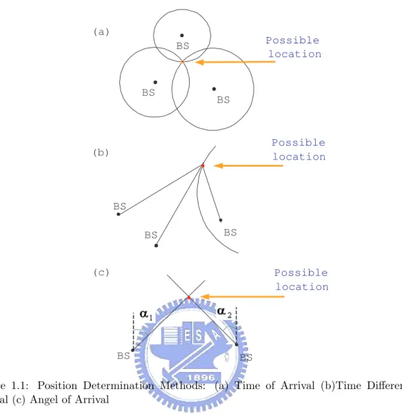
The well-adapted technology for the satellite-based location estimation method is to utilize the Global Positioning Systems (GPSs). It measures the Time-Of-Arrival (TOA) of the signals coming from different satellites. The TOA scheme determines the mobile device position based on the intersection of the range circles, as shown in Fig. 1.1a. Since the propagation time of the radio wave is directly proportional to its traversed range, multiplying the speed of light to the time can obtain the range from the mobile device to the communicating Base Station (BS). It is noted that two range measurements provide an ambiguous fix, while three

(5)

Possible location BS BS BS (a) (b) (c) BS Possible location BS BS Possible location BS BS

Figure 1.1: Position Determination Methods: (a) Time of Arrival (b)Time Difference of Arrival (c) Angel of Arrival

measurements determine a unique position. The same principle is used by GPS, where the circles become the spheres in space and the fourth measurement is required to obtain the 3-D position for mobile device.

The network-based location estimation schemes have been widely proposed and employed in the wireless communication system. These schemes locate the position of the MS based on the measured radio signals from its neighborhood BSs. The representative algorithms for the network-based location techniques are the Time Difference-Of-Arrival (TDOA) and the Angle-Of-Arrival (AOA). The TDOA scheme determines the mobile device position based on the trilateration, as shown in Fig. 1.1b. The scheme uses time difference measurements rather than absolute time measurements as TOA dose. It is often referred to as the hyperbolic system

(6)

because the time difference is converted to a constant distance difference to two base stations (as foci) to define a hyperbolic curve. The intersection of two hyperbolas determines the mobile device position. Therefore, it utilizes two pairs of BSs for positioning. The accuracy of the scheme is a function of the relative base station geometric locations. For the network-based systems, it also requires either precisely synchronized clocks for all transmitters and receivers or a means to measure these time differences.

The AOA technique determines the mobile device position based on triangulation, as shown in Fig. 1.1c. It is also called direction of arrival in some literature. The intersection of two directional lines of bearing defines a unique position, each formed by a radial from a BS to the mobile device in the 2-D space. This technique requires a minimum of two BSs to determine a position. If available, more than one pair can be used in practice. However, since directional antennas or antenna arrays are required, it is generally difficult to realize the AOA technique at the mobile device.

It has been studied in several research [4]- [6] that the performance of the location es-timation techniques listed above varies under different environments, where each technique provides its advantages and limitations. In order to provide consistent location estimation accuracy under different circumstances, a hybrid location estimation scheme is proposed in part I of this thesis.

On the other hand, two algorithms are proposed in part II of this thesis for enhanced wireless location estimation. As mentioned before, the major methods for the location esti-mation techniques are the TOA, TDOA, and the AOA techniques. The equations associated with the location estimation schemes are inherently nonlinear. Some different linear methods have been proposed to obtain an approximate location. However, the methods are primar-ily feasible for location estimation under Line-Of-Sight (LOS) environments. In part II, an Geometry-constrained Location Estimation (GLE) algorithm and a location estimation with the Virtual Base Stations (VBS) are proposed to obtain location estimation of the MS, espe-cially for NLOS environments.

(7)

mathematic modeling, the sources of ranging errors, and other existing location estimation algorithms, is briefly described in chapter 2. The overview of the proposed hybrid location estimation algorithm can be obtained in chapter 3. Chapter 4 presents the system architecture of the proposed algorithm. The proposed hybrid location estimation, filtering, and fusion techniques are described in chapter 5. Chapter 6 illustrates the performance evaluation of the proposed hybrid location estimation scheme in simulations. Chapter 7 shows the overview of the proposed GLE and VBS algorithms. Chapter 8 describes both the GLE and VBS algorithms in detail. The performance of the proposed two schemes are conducted in chapter 9 via simulations. Chapter 10 draws the conclusions.

(8)

Chapter 2

Related Work

2.1 Mathematical Modeling

In this section, the mathematical models for the TOA, TDOA, and AOA measurements are

presented. The TOA measurement t_` from the `th _{BS is obtained by}

t`= r_c` = 1_cζ`+ n` ` = 1, 2, ...n (2.1)

where c is the speed of light, and r_` represents the measured relative distance between the

MS and the `th _{BS contaminated with the TOA measurement noise n}

`. The noiseless relative

distance ζ` between the MS and the `th BS can be obtained as

ζ_` = kx − x_`k (2.2)

where x = (x, y) represents the MS’s position, and x` = (x`, y`) is the location of the `th BS

in the 2-D setting; while in the 3-D formulation, x = (x, y, z) and x` = (x`, y`, z`). On the

other hand, the cellular-based TODA measurement ti,j is obtained by computing the time

difference between the MS w.r.t. the ith and the jth BSs:

(9)

where n_i and n_j represent the measurement noises from the MS to the ith _{and the j}th _BSs.

Since it is assumed that the antenna arrays at the home BS can only measure the incoming signals along the x and y directions, the AOA measurement θ of the cellular system is obtained as

θ = tan−1(y − y1

x − x1

) + n_θ (2.4)

where θ represents the horizontal angle between the MS and its home BS. (x1, y1) is the

horizontal coordinate of the home BS, and nθ is measurement noise associated with θ.

2.2 Sources of Ranging Errors

The location accuracy reduces due to the influence of the measurement noises. Several main sources of ranging errors are described in this section and this content is referred to [7]. Non-Line-of-Sight Errors

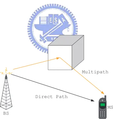
In dense urban environment, there may be no direct path from the MS to the BS as shown in Fig. 2.1. Due to reflection and diffraction, the propagating wave may actually travel excess path lengths on the order of hundreds of meters and the direct path is blocked. This phenomenon, which we refer to as the NLOS error, ultimately translates into a biased estimate of the mobile’s location. This problem has been recognized as a killer issue for mobile location. In order to mitigate the effect of the measurement bias, it is necessary to develop location algorithms that are robust to the NLOS error.

Multipath Errors

Multipath effects are caused by reflected signals entering the receiver antenna along with direct path signal, as shown in Fig. 2.2. Since the reflected path is longer than the direct path, the multipath signal blurs the peak of the direct signal at the output of the receiver correlation channel and distorts the pseudorange measurement.

(10)

MS

BS

Direct

Path NLOS Path

Figure 2.1: Geometry of the NLOS Error

BS

MS Direct Path

Multipath

(11)

Receiver Measurement Processing

Advances in digital processing technology have enabled the implementation of small, afford-able multiple channel receivers for parallel tracking of more than the minimum reference points for navigation solutions. This technology, in conjunction with advances in the speed and precision of microprocessor computations, has resulted in great reductions in receiver range measurement processing errors.

2.3 Studies on Existing Location Estimation Algorithms

Different location estimation schemes have been proposed to acquire the MS’s position. Var-ious types of information (e.g. the signal traveling distance, the received angle of the signal, or the Receiving Signal Strength (RSS)) are involved to facilitated the algorithm design for location estimation. The primarily objectives in most of the location estimation algorithms are to obtain higher estimation accuracy with promoted computational efficiency. The super-resolution (or high-resoluction) schemes are proposed as in [8] - [11]. The scheme studied in [8] considers arbitrary-located antennas and a particular covariance matrix within a noisy environment. The covariance matrix is composed of various types of properties, including gain, phase, frequency, polarization, and AOA information. The subspace method is pro-posed in the scheme generates these component estimates of the covariance metrix based on an eigen-analysis or eigen-composition. The most well-known super-resolution algorithm is the MUltiple SIgnal Classification (MUSIC) [9], It is experimentally illustrated to be a robust solution for location estimation, especially for a near-far environment. However, it has also be shown in [10] and [11] that the drawbacks of the MUSIC approach include (i) comparably high sensitivity to large noise and (ii) its complexity in computation.

The beamforming system is a space-time processor that operates on the output of a sensor array. It provides spatial filtering capability by enhancing the amplitude of a coherent signal associated with surrounding noises. Since the conventional beamforming technique is sensitive to the estimation error for the MS’s position, a combination of localization and beamforming is proposed as in [12]. It increases the robustness to location errors without sacrificing the

(12)

computation efficiency. An enhanced algorithm for simultaneous multi-source beamforming and adaptive multi-target tracking is studied in [13]. The correlation between the adaptive minimum variance beamforming and the optimal source localization is also investigated and developed as in [14].

Instead of exploiting the spatial and temporal information of the signal, the location fingerprinting technique locates the MS based on the the RSS [15] [16]. The technique involves both the off-line and the on-line phases. A location grid that is related to a signal signature database for a specific service area is developed in the off-line phase; while a measured RSS vector at the MS is delivered to the central server to compare with the location grid in the on-line phase. In addition, a hybrid algorithm which combines the RF propagation loss model is proposed to both mitigate the requirement of the training data and to adjust the configuration changes [17]. On the other hand, the ray-tracing and ray-launching techniques are the two ray optical approaches for location estimation. The radio signals that are launched from a transmitter and reflected or diffracted by various objects are aggregated in a receiver. The field strength and the signal propagation can therefore be predicted [18]; while [19] proposed an efficient algorithm for prediction. The three dimensional indoor radio propagation models are developed in [20] and [21]. Experimental formulas from extensive measurements of urban and suburban propagation losses are studied as in [22] [23].

There are also different approaches adopting linearized methods to acquire the computing efficiency while obtaining an approximate estimation of the MS’s position. The Taylor Series Expansion (TSE) method was utilized in [24] to acquire the location estimation from the TDOA measurements. The method requires iterative processes to obtain the location estimate from a linearized system. The major drawback of this method is that it may suffer from the convergence problem due to an incorrect initial guess of the MS’s position. The two-step LS method was adopted to solve the location estimation problem from the TOA [25], the TDOA [26], and the TDOA/AOA measurements [27]. It is an approximate realization of the Maximum Likelihood (ML) estimator and does not require iterative processes. The two-step LS scheme is advantageous in its computational efficiency with adequate accuracy for

(13)

location estimation. However, the scheme is demonstrated to be feasible for acquiring the MS’s position under the LOS situations.

Instead utilizing the Circular Line Of Position (CLOP) methods (e.g. the TSE and two-step LS schemes), the Linear Line Of Position (LLOP) approach is presented as a new inter-pretation for the cell geometry from the TOA measurements. Since two TOA measurements that intersect at two points will generate a connecting line, two independent lines will be created by using three BSs in the scenario of two-dimensional location estimation. Therefore, the LS method can be adopted to estimate the location of the MS. The detail algorithm of the LLOP approach can be obtained by using the TOA measurements as in [28], and the hybrid TOA/AOA measurements in [29].

Some well-known schemes are improved continuously in order to achieve higher accu-racy or promote the computational efficiency. The famous linear time-based algorithms, the Taylor-Series Estimation (TSE) [24], the two-step LS method, and the Linear Line-of-Position (LLOP) [28], are briefly described in the following subsection. For simplification, the thesis described the TSE, two-step LS and LLOP methods in two-dimensional plane.

2.3.1 Taylor-Series Estimation

The content of this section will show the Taylor-Series Estimation (TSE), which is available in [24].

Assuming that (x, y) is the position of the MS, (x`, y`) is the position of the `th base

station and r` is the TOA measurement from the base station `. Since in practice, especially

in urban or in mountainous areas, the signals from the mobile device are usually unable to arrive at the base stations directly (or in the oppositive direction), they always take a longer path than the direct one. So by incorporating the influences of NLOS propagation on the location estimation, there exists

f`(x, y, x`, y`) = ζ`= r`− n` (2.5)

(14)

mea-surement noise and is statistically distributed. We take the noises to have zero-mean values

< n_`>=0 and nij =< ninj > is the i − jth term in the covariance matrix

Q = [nij]

If the xv, yv are guesses of the true variable position, write

x = xv+ δx y = yv+ δy (2.6)

and expand f_` in Taylor’s series keeping only terms below second order

f`v + a`1δx+ a`2δy ' r`− n` (2.7)

where

f`v = f`(xv, yv, x`, y`)

a`1= ∂f`/∂x|xv,yv a`2= ∂f`/∂y|xv,yv

and the approximate relations of 2.7 can be written as

Aδ ' z − n (2.8) where A =          a11 a12 a21 a22 . . aN 1 aN 2          δ =    δx δy    z =          r1− f1v r2− f2v . rN − fN v          n =          n1 n2 . nN         

(15)

δ = (ATQ−1A)−1ATQz (2.9)

Thus, to estimate the position of the MS, compute δ_x, δ_y with (2.9), replace

xv ← xv+ δx yv ← yv+ δy (2.10)

in (2.9), and repeat the computations. The iterations will have converged when δx and δy are

essentially zero.

2.3.2 Two-Step Least Square Location Algorithm

The content of this section will show the Two-step Least Square (two-step LS) location algo-rithm for TOA measurements and it can be obtained in [25]. For simplification, the two-step LS method will be described for TOA measurements in a two-dimensional (2-D) plane. The two-step LS method for TDOA measurements can be derived from the similar concept.

Assuming that (x, y) is the position of the mobile device, (x`, y`) is the position of the

`th _{base station and r}

` is the TOA measurement from the base station `. Since in practice,

especially in urban or in mountainous areas, the signals from the mobile device are usually unable to arrive at the base stations directly (or in the oppositive direction), they always take a longer path than the direct one. So by incorporating the influences of NLOS propagation, killer issue for location estimation, on the location estimation, there exists

r2_` ≥ (x`− x)2+ (y`− y)2 = κ`− 2x`x − y`y + x2+ y2 ` = 1, 2, ...N (2.11)

where κ_` = x2

` + y`2, r` = ct` is the measured distance between the MS and the `th base

station, and c is the speed of light. And by defining a new variable β = x2_{+ y}2_{, we rewrite}

(2.11) through a set of linear expressions

(16)

Let x_a= [x y β]T _{and express (2.12) in matrix form} Hxa≤ J (2.13) where H =          −2x1 − 2y1 1 −2x2 − 2y2 1 . . . −2xN − 2yN 1          J =          r2 1− κ1 r2 2− κ2 . r2 N− κN         

With measurement noise, the error vector is

ψ = J − Hx_a (2.14)

When r` can be expressed as ξ`+ cn`, the error vector ψ is found to be

ψ = 2cBn + c2n ¯ n

B = diag{ξ1, ξ2, ..., ξN} (2.15)

The symbol ¯ represents the Schur product (element-by-element product). In addition, the

second term on the right of (2.15) can be ignored since the condition cn` ≤ ξ` is usually

satisfied. As a result, ψ becomes a Gaussian random vector with covariance matrix given by

Ψ = E[ψψT] = 4c2BQB (2.16)

Q is the covariance matrix of measured noise, and ξ1,...,ξN are denoted as the true values of

distances between the sources and the receiver. The element xa are related by the equation,

β = x2 + y2, which means that (2.13) is still a set of nonlinear equations in two variables

x and y. The approach to solve the nonlinear problem is to first assume that there is no

relationship among x, y and β. That can then be solved by Least Square (LS). The final solution is obtained by imposing the known relationship to the computed result via another

(17)

LS computation. This two step procedure is an approximation of a true ML estimator. By

considering the elements of xa independent, the ML estimator of xa is

xa = arg min{(J − Hx )TΨ−1(J − Hx )}

= (HTΨ−1H)−1HTΨ−1J (2.17)

The covariance matrix of xais obtained by evaluating the expectations of xaand xaxTa from

(2.17). The covariance matrix of x_a can be calculated as [26]

cov(xa) = (HTΨ−1H)−1 (2.18)

Since we have used the independent supposition of variables x, y, and β in the estimation

of xathough the variable β is dependent on the variable x and y, we should revise the results

as follows. Let the estimation errors of x, y, and β be e1, e2, and e3. Here and below, denote

the ith _{entry of a matrix M as [M ]}

i; then the entries in vector xa become

[xa]1 = xo+ e1 (2.19a)

[xa]2 = yo+ e2 (2.19b)

[xa]3 = βo+ e3 (2.19c)

where xo, yo, and βo are denoted as the true values of x, y, and β. Let another error vector

ψ_b = J_b− H_bx_b (2.20) where Hb=      1 0 0 1 1 1      Jb=      [xa]21 [xa]22 [xa]3     

(18)

and x_b=   x 2 y2  

. Substituting 2.19a- 2.19c into 2.20, we have

[ψ]1 = 2xoe1+ e21 ≈ 2xoe1

[ψ]2 = 2yoe2+ e22≈ 2yoe2

[ψ]₃ = e₃

Obviously, the above approximations are valid only when the errors e1, e2, and e3 are fairly

small. Subsequently, the covariance matrix of ψb is

Ψ_b = E[ψ_bψT_b] = 4B_bcov(x )B_b

Bb = diag{xo, yo, 0.5} (2.22)

As an approximation, elements xoand yoin matrix x can be replaced by the first two elements

x and y in xa. Similarly, the ML estimate of xb is given by

xb = (HTbΨ−1b Hb)−1HTbΨ−1b Jb (2.23)

≈ (HT_bB−1_b (cov(x )a)−1B−1_b Hb)−1 (2.24)

• (HT_bB−1_b (cov(x )a)−1B−1_b )Jb (2.25)

So the final position estimation x = [x y]T _is

x =√x_b, or x = −√x_b (2.26)

Here the sign of x should coincide with the sign of [xa]1 calculated by solving 2.17, and the

sign of y coincides with the sign of [xa]2.

The complete derivation of the two-step LS for TOA measurements is shown above. In addition, the two-step LS method can be adopted to estimate MS location from the TDOA [26], and the TDOA/AOA measurements [27]. The following two subsections describe the 3-D

(19)

TOA location estimation for the satellite-based system, and the 3-D TDOA/AOA location estimation algorithm for the cellular network.

2.3.3 Linear Line-of-Position

The content of this section will show the linear Line-of-Position (LLOP) and it can be referred to [28].

The TOA location method measures the ranges between MS and BSs. This range between

the `th _{BS and the MS can be expressed as}

ζ` =

p

(x`− x)2+ (y`− y)2 (2.27)

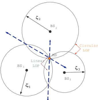
where (x, y) is the position of the MS, (x`, y`) is the position of the `th BS. The relationship

between the ranges for three BSs, their location, and the position of the MS are shown in Fig. 2.3 in two dimensions.

The Linear Line-of-Position (LLOP) method is based on the observations of Fig. 2.3. In-stead utilizing circular LOPs, LLOP presents the approach of the linear LOPs (LLOP), a new interpretation of the geometry of TOA location. Since two TOA measurements intersections at two points generate a line, the least number of BSs (i.e. 3)used to estimate the location of MS in 2D scenarios will produce two independent lines. As indicated in the figure, the new LLOPs also intersect at the location of the MS.

To determine the equations for the new linear LOPs, we must start with the original LOP equations, given in (2.27) for ` = 1, 2, 3. The lines which pass through the intersection of the three circular LLOPs can be obtained by squaring and differentiating the ranges in (2.27) for

` = 1, 2 and ` = 1, 3 which result in

(x2− x1)x + (y2− y1)y = 1₂(x22− x21+ ζ12− ζ22) (2.28)

(x₃− x₁)x + (y₃− y₁)y = 1 2(x

2

3− x21+ ζ12− ζ32) (2.29)

(20)

BS BS BS 1 2 3 Circular LOP Linear LOP MS

Figure 2.3: The Geometry of TOA-Based Location with Circular LOPs and Linear LOPs and (2.29). The location of the MS (x, y) can be obtained as

x = (y2− y1)C2− (y3− y1)C1 (x3− x1)(y2− y1) − (x2− x1)(y3− y1) (2.30) y = (x2− x1)C2− (x3− x1)C1 (x2− x1)(y3− y1) − (x3− x1)(y2− y1) (2.31) where C1 = (x22− x21+ ζ12− ζ22) C2 = (x23− x21+ ζ12− ζ32)

The previous section developed the location geometry for locating a MS in 2-D with three BSs. When there are more than the minimum number (i.e. greater than three BSs in 2-D and when there are measurement errors in the TOAs, two approaches to algorithm development can be taken: an intersection solution (geometry based) and a least squares solution.

(21)

Intersection Solution

This approach can be generalized for N total BSs where independent N − 1 lines can be produced from the intersections of the N circles. These N − 1 linear LOPs could then be used to compute the intersection points. All of the intersections of the independent N − 1 lines

could be used to obtain (N −1)(N −2)₂ intersection points. As a result, the location of the MS

could be found from the mean of the intersection points or the centroid of a polygon formed by these points.

Least Squares Solution

An alternative approach to the solution of geometric equations is to compute the position of the MS using a least squares when the number of the received BSs (N ) is more than three. Each of the independent N − 1 lines is the form (shown as in (2.28)- (2.29))

a`,1x + a`,2y = aT`x = b` (2.32)

for the `th _{line, where a}

` = [a`,1, a`,2]T and x = [x, y]T. The system of equations describing

all of the lines can be written in matrix form as

Ax = b (2.33)

where AT = [a1 a2...aG] and b = [b1 b2...bG]T, and G is the number of lines used. Due to the

measurement errors , LS estimate is used to solve a LS solution

ˆ

x = (ATA)−1ATb (2.34)

This algorithm is obviously much less difficult than the geometric one since there is no need to compute intersections of many lines.

(22)

Part I

Hybrid Location Estimation and

Tracking System for Mobile Devices

(23)

Chapter 3

Overview

In general, the location estimation schemes can be classified into (i) the satellite-based and

(ii) the network-based location estimation algorithms. The well-adapted technology for the satellite-based location estimation method is to utilize the Global Positioning Systems (GPSs). The representative algorithms for the network-based location techniques are the Time Difference-Of-Arrival (TDOA) and the Angle-Of-Arrival (AOA). It has been studied in [4] that the performance of the location estimation techniques listed above varies under dif-ferent environments. Due to weak incoming signals or shortage of signal sources (e.g. at rural area), the network-based (i.e. TDOA, AOA) methods result in degraded performance for the location determination of mobile devices [5] [6]. On the other hand, the major problem for the satellite-based method is that the performance considerably degrades while the satellite signals are severely blocked (e.g. at urban valley area).

In order to achieve better accuracy for location estimation, a hybrid approach should be considered to satisfy the requirements under different environments. In this thesis, a hybrid location estimation and tracking system is proposed for the Mobile Stations (MSs). The proposed location estimation scheme determines the MS’s location by combining the outcomes from both the network-based and the satellite-based techniques. In addition to the longitude (x) and latitude (y) of the MS can be estimated, the altitude information (z) of the MS is obtainable from the proposed system. The two-step Least Square (LS) method [25]- [27]

(24)

is utilized to estimate the MS’s position based on the measurements. The Kalman filtering technique [30] is exploited to smooth out the measurement noises and to track the position and velocity of the MS. The Bayesian Inference Model [31] [32] is adopted as the fusion mechanism to acquire the final position estimate from the GPS system and the cellular networks. The performance of the proposed hybrid location estimation scheme is evaluated via simulations under different environments.

(25)

Chapter 4

System Architecture

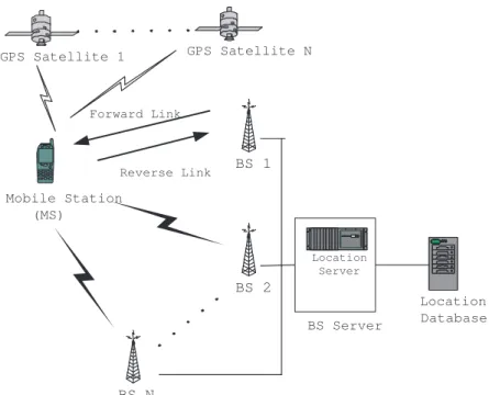
Fig. 4.1 shows the schematic diagram of the system architecture for the proposed hybrid location estimation. The hybrid system combines the signals coming from both the satellies and the cellular networks. In order to obtain the TOA measurements from the satellites, it is assumed that each MS is equipped with a GPS receiver. On the other hand, the proposed hybrid system adopts the following features from the 3GPP standard [33] [34]:

1. Each Base Station (BS) has a forward-link pilot channel that continuously broadcast its pilot signal in order to provide timing and phase information for all the MS in this cellular network..

2. Each BS has a dedicated reverse-link pilot channel from the MS to provide initial ac-quisition, time tracking, and power control measurements..

3. Each BS is equipped with antenna arrays for adaptive beam steering in order to facilitate the AOA measurements. As shown in Fig. 4.1, the TDOA measurements are conducted at the MS by obtaining the signals via the forwrd-link pilot channels from the BSs. The AOA signals are transmitted from the MS to the BSs using the reverse-link pilot channel. The AOA measurements are performed at the BS using its antenna arrays for two-dimensional adaptive beam steering. In order to avoid signal degradation due to the near-far effect, it is assumed in the proposed system that only the home BS provides

(26)

Mobile Station (MS) BS 1 BS N BS 2 GPS Satellite N Forward Link Reverse Link GPS Satellite 1 Location Database BS Server Modem Bank Location Server

Figure 4.1: The Schematic Diagram of the Hybrid Mobile Location Scheme the capability of the AOA measurements.

As stated in the 3GPP standard, the location determination of the MS can either be MS-Based or MS-Assisted. The choice between these two types of system depends on the requirement of the communication bandwidth and the computation power of the MS. The hy-brid location estimation scheme proposed in this paper can be applied to either MS-Assisted or MS-Based system. The following two subsections describe the proposed system architectures based on these two types of system:

The Mobile-Assisted System

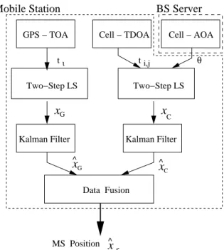
The left schematic diagram of Fig. 4.2 shows the proposed hybrid algorithm that implements on the MS-Assisted positioning system. This type of architecture is suitable for the MS with insufficient computation capability. The following steps describe the procedures of the proposed scheme for the MS-Assisted system:

1. The GPS-equipped MS receives signals from the satellites and conducts TOA

(27)

GPS − TOA Cell − TDOA Kalman Filter Mobile Station t Cell − AOA Two−Step LS Kalman Filter MS Position _x^ f xG ^ x ^ C ι x_G x C i,j t θ BS Server Two−Step LS Data Fusion

Figure 4.2: The Hybrid Location Estimation Scheme based on the Mobile-Assisted System .

three-dimensional position (i.e. xG=[xG yG zG]T) of the MS using the two-step LS

method. On the other hand, the TDOA measurement are calculated at the MS by obtaining signals from its home Base Station (BS) and the neighboring BSs via the forward-link pilot channel

2. These two sets of information, the location estimation (xG) and the TDOA

measure-ments (ti,j), are transmitted back to the home BS via the reverse-link pilot channel.

3. The AOA measurement (θ) is conducted at the home BS by receiving the signals from the MS via the reverse-link channel.

4. The location server at the home BS performs location estimation by combining the AOA and the TDOA measurements. The two-step LS method is utilized to estimate

three-dimensional position (x_C) of the MS.

5. The BS location server performs Kalman filtering technique to smooth out the measure-ment noises and to track the position data both from the TOA and the TDOA/AOA channels.

(28)

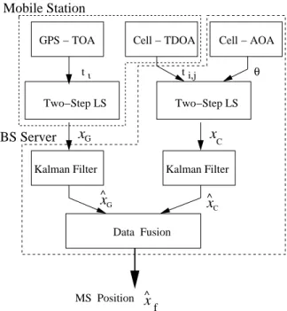
GPS − TOA Cell − TDOA Kalman Filter Mobile Station t Cell − AOA Two−Step LS Kalman Filter MS Position _x^ f xG ^ x ^ C ι xG x_C i,j t θ Two−Step LS Data Fusion BS Server

Figure 4.3: The Hybrid Location Estimation Scheme based on the Mobile-Based System .

6. Data Fusion is performed to incorporate both the means (ˆx_G and ˆx_C) of the filtered

estimations (ˆx_G and ˆx_C) from the TOA and the TDOA/AOA measurements based on

their signal variations. The fused position estimate (ˆx_f) of the MS can be obtained.

The Mobile-Based System

The right schematic diagram of Fig. 4.3 shows the proposed scheme for the MS-Based po-sitioning system. This type of architecture is suitable for the MS that possesses adequate computation capability. The following procedures describe the proposed algorithm for the MS-Based system:

1. The AOA measurement (θ) is obtained from the home BS and is transmitted to the MS

via the forward-link pilot channel. The TDOA measurements (t_i,j) is computed within

the MS using the signals coming from the MS’s home and neighboring BSs.

2. The GPS-equipped MS receives signals from the satellites and provides location estimate

(29)

3. The MS performs location estimate (x_C) by combining the TDOA and the AOA mea-surements using the two-step LS method.

4. The Kalman filtering techniques for both the TOA and the TDOA/AOA channels are

performed at the MS to obtain the location estimates, ˆx_G and ˆx_C. The final position

estimation (ˆx_f) is acquired after the fusion results from the mean values of the location

(30)

Chapter 5

The Location Estimation and

Tracking Algorithms

As described in chapter 4, the proposed hybrid location estimation and tracking system con-sists of three major components for location estimation and filtering: the two-step LS method, the Kalman filtering technique, and the data fusion. The following subsections describe these three components.

5.1 Two-Step Least Square Location Algorithm

Different approaches have been proposed for wireless location estimation in previous stud-ies [24] [25] [26] [27]. The Taylor serstud-ies expansion method proposed in [24] was utilized to acquire the location estimation from the TDOA measurements. The method requires iterative processes to obtain the location estimate from a linearized system. The major drawback of this method is that it may suffer from the convergence problem due to the initial position guess. The two-step LS (Least Square) method, an approximate realization of the Maximum Likelihood (ML) estimator, was adopted to solve the location estimation problem and does not require iterative processes. In addition to estimating the two-dimensional position of the MS as in the previous research, the two-step LS method is applied in the proposed hybrid system to calculate the 3-D location of the MS.

(31)

3-D TOA Location Estimation

In order to solve for the two-step LS problem from the TOA measurements, it is assumed that signals coming from at least four satellites are available. The 3-D TOA measurements as described in (2.1) can be rewritten as

Hx = J (5.1) where x = · x y z β ¸_T H =          −2x1 − 2y1 − 2z1 1 −2x2 − 2y2 − 2z2 1 . . . . −2xN − 2yN − 2zN 1          J =          r2 1 − κ1 r2 2 − κ2 . r2_N− κN         

It is noted that β = x2 _{+ y}2_{+ z}2 _{and κ}

` = x2` + y`2+ z`2 for ` = 1, 2, ...N . The concept

of the two-step LS method is to acquire an intermediate location estimate in the first step by assuming that x, y, z and β are not correlated. The second step of the method releases this assumption by adjusting the intermediate result to obtain an improved location estimate,

xG=[xG yG zG]T. The details of the two-step LS method is shown in [25].

3-D TDOA/AOA Location Estimation

To solve for the two-step LS problem for the cellular-based system, the home BS should provide both the TOA and AOA measurements, while three additional TOA measurements are assumed to be obtainable from other BSs. The 3-D TDOA and AOA measurements as in

(32)

(2.3) and (2.4) can also be rewritten as (8.5), where the matrices H and J becomes H = −             x2− x1 y2− y1 z2− z1 r2,1 x3− x1 y3− y1 z3− z1 r3,1 . . . . xN − x1 yN − y1 zN− z1 rN,1 − sin θ cos θ 0 0             J =1 2             r2 2,1− κ2+ κ1 r2 3,1− κ3+ κ1 . r2 N,1− κN+ κ1 2x1sin θ − 2y1cos θ            

In both matrices, the AOA components are computed based on the geometric approximation as described in [27]. The two-step LS method is applied to obtain the location estimates from the TDOA/AOA measurements.

5.2 Kalman Filtering

The content of this section will show the Kalman filtering and it can be referred to [28]. The Kalman filtering technique [30] is employed in the proposed scheme for post-processing of measured signals. It provides the capabilities of range measurement, smoothing, and noise mitigation for the TOA and the TDOA/AOA data. Furthermore, the Kalman filter can also be utilized for trajectory tracking of the MS. The state equation for the Kalman filter can be written as

ˆ

x_k= Aˆx_k−1+ Γw_k−1 (5.2)

The state vector, ˆxk=[ˆxk yˆkzˆkvˆxk ˆvyk vˆzk]T, is defined as the estimated position and velocity

of the MS. The state matrix A represents the state change between the current time step k

(33)

Q = σ2 eI, and A =   I 4tI 0 I   _{Γ =}   0 4tI  

The measurement process is described as

xk= Bˆxk+ ek (5.3)

where x_k=[x_k y_k z_k]T _{represents the measured data coming from the two-step LS algorithm.}

The matrix B relates the state vector ˆxk to the measurements xk and B = [I 0]. wk

represent the measurement noises with covariance matrix R = σ2

ˆ

xI. (5.4)- (5.8) show the

iteration operation of the Kalman filter

ˆ x_k,k−1 = Aˆx_k−1,k−1 (5.4) Ck,k−1 = ACk−1,k−1AT + ΓQΓT (5.5) K = Ck,k−1BT(BCk,k−1BT + R−1)T (5.6) C_k,k = C_k,k−1− KBC_k,k−1 (5.7) ˆ xk,k = ˆxk,k−1+ K(xk− BAˆxk−1,k−1) (5.8)

where K is the kalman gain and C_k,k is the covariance matrix of the ˆx_k,k.

As shown in Fig. 4.2, the Kalman filtering technique is applied to both the TOA and the TDOA/AOA channels. The effectiveness of the Kalman filter will be illustrated in the next section via simulations.

5.3 Data Fusion

The main functionality of data fusion is to merge disparate types of information in order to enhance the position accuracy. By merging the TOA and the TDOA/AOA estimations, the resulting data provides feasible location estimates under different environments (i.e. urban,

(34)

suburban, and rural). The fusion process used in this paper is based on the Bayesian Inference model [31] [32], which improves an estimate with known statistics. The fused position estimate ˆ

x_f and its variance σ2

f are obtained as follow:

ˆ xf = σ2 G σ2 G+ σC2 ˆ x_C+ σ 2 C σ2 G+ σ2C ˆ x_G (5.9) σ_f2 = 1 σ_C−2+ σ_G−2 (5.10)

where ˆx_C=[ˆx_C ˆy_C ˆz_C]T _{represents the mean value of the location estimate ˆ}_x

C from the

TDOA/AOA channel; ˆx_G=[ˆx_G ˆy_G ˆz_G]T _{is the mean value of the location estimate ˆ}_x

G from

(35)

Chapter 6

Performance Evaluation

6.1 The Noise Model

Different noise models [25] [27] [37] [38] for the satellite-based and network-based system are considered in the simulations. The models for measurement noises will be described as follows: The Noise Model of TOA Measurements for the Satellite-based System

The probability distribution of the noise model for the satellite-based system, p_n`(τ ), is

ob-tained as

pn`(τ ) = τ_cg · Ug(τ ) (6.1)

where Ug(τ ) represents a uniform distribution function on the interval [0, 1]. τg is assumed

(36)

TABLE I

Parameters for Noise Models under Different Environments

Environment τg(m) τa τm (µs)

Urban 140 9o 0.4

Suburban 90 7o _0.3

Rural 40 5o 0.1

The Noise Model of AOA Measurements for the Network-based System

The probability distribution of the noise model for the AOA measurements, pnθ(τ ), is assumed

as

pnθ(τ ) = τa· Ua(τ ) (6.2)

where Ua(τ ) is a uniform distribution function on the interval [0, 1]. The selection of the τa

is also dependent on the environment.

The Noise Model of TOA/TDOA Measurements for the Network-based System The model for the measurement noise of the TOA signals is selected as the Gaussian distribu-tion with zero mean and 10 meters of standard deviadistribu-tion. On the other hand, an exponential

distribution pn`(τ ) is assumed for the NLOS noise model of the TOA measurements as pnk(τ )

as p_nk(τ ) =      1 τke −τ τk τ > 0 0 otherwise (6.3)

for ` = 1, 2,...N. τ` = τmζ`ερ is the RMS delay spread between the `th BS to the MS; τm is

the median value of τ` whose value depends on the various environment. ε is the path loss

exponent which is assumed to be 0.5, and the factor for shadow fading ρ is set to 1 in the simulations. On the other hand, the noise model of the TDOA measurements is described as

(37)

the exponential distribution for k = i, j.

6.2 Simulation Parameters

Simulations are performed to show the effectiveness of the proposed location estimation scheme. In the simulations, signals from four satellites and four BSs are assumed available for estimating the position of the MS. The positions of the four satellites are located at (0, 0, 20000), (8000, 16000, 9000), (12000, 9000, 7000), and (8000, 7000, 17000) in kilometers. The home BS is located at (0, 0, 330) in meters, while the positions of the other three neighboring

BSs are at (-1000, 1000√3, 350), (1000, 1000√3, 370), and (2000, 0, 340) all in meters. The

MS is assumed to travel at a constant speeds of (3, 4, 0) m/sec along the x, y, and z direc-tions, i.e. (x, y, z) = (27 + 3t, 36 + 4t, 300) in meters. The total traveling time of the MS

is assumed to be 100 seconds. τg, Ua(τ ), and τm are assumed to be constant values varying

under different types of environment as given in Table I.

6.3 Simulation Results

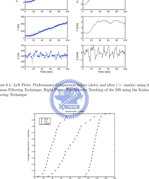
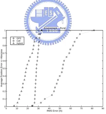
The effectiveness of using the Kalman filtering technique can be observed from Fig. 6.1. It eliminates measurement noises and tracks the MS’s position and velocity in the longitude, latitude, and altitude directions. Fig. 6.2 - Fig. 6.4 shows the performance comparison between the proposed hybrid location estimation system, the satellite-based system, and the cellular-based system under urban, suburban, and rural environments. It can be seen that

the RMS error of the MS’s position (i.e. ∆P_f = [(x_f− x)2_{+ (y}

f− y)2+ (zf− z)2]

1

2) obtained

from the hybrid scheme is smaller comparing with that from the other two approaches. It is also noted that the estimation error acquired from the satellite-based system has the worst performance comparing with the other two systems in the urban area; while the cellular-based system causes degraded results in the rural area. The hybrid system is capable of adjusting itself to accommodate different situations, which provides consistent performance comparing with the satellite-based and the cellular-based systems.

(38)

0 20 40 60 80 100 −200 0 200 400 MS position X (m) 0 20 40 60 80 100 0 200 400 600 Y (m) 0 20 40 60 80 100 270 280 290 300 310 Z (m) Time (sec) 0 20 40 60 80 100 −2 0 2 4 6 MS velocity X (m/s) 0 20 40 60 80 100 −2 0 2 4 6 Y (m/s) 0 20 40 60 80 100 −4 −2 0 2 Z (m/s) Time (sec)

Figure 6.1: Left Plots: Performance Comparison before (dots) and after (’+’ marks) using the Kalman Filtering Technique; Right Plots: The Velocity Tracking of the MS using the Kalman Filtering Technique . 0 20 40 60 80 100 120 140 160 180 0 0.1 0.2 0.3 0.4 0.5 0.6 0.7 0.8 0.9 1

Average Position Error <= Abscissa

RMS Error (m) Environment − Urban

GPS Cell Hybrid

Figure 6.2: Performance Comparison between the Hybrid System, the Satellite-based System, and the Cellular-based system under Urban Environment

(39)

0 20 40 60 80 100 120 0 0.1 0.2 0.3 0.4 0.5 0.6 0.7 0.8 0.9 1

RMS Error (m) Environment − Suburban

GPS Cell Hybrid

Figure 6.3: Performance Comparison between the Hybrid System, the Satellite-based System, and the Cellular-based system under Suburban Environment

0 10 20 30 40 50 60 70 80 90 0 0.1 0.2 0.3 0.4 0.5 0.6 0.7 0.8 0.9 1

RMS Error (m) Environment − Rural

GPS Cell Hybrid

Figure 6.4: Performance Comparison between the Hybrid System, the Satellite-based System, and the Cellular-based system under Rural Environment

(40)

Part II

Enhanced Wireless Location

Estimation Algorithms

(41)

Chapter 7

Overview

A variety of wireless location techniques have been studied and investigated [1]- [3]. The network-based location estimation schemes have been widely exploited in the wireless com-munication system. These schemes locate the position of the MS based on the measured radio signals from its neighborhood BSs. The major time-based methods for the network-based lo-cation estimation techniques are the TOA, and the TDOA. The TOA scheme measures the arrival time of the radio signals coming from different wireless BSs; while the TDOA scheme measures the time difference between the radio signals.

Since the equations accompanied with the network-based location estimation schemes are inherently nonlinear, it is required to adapt approximation techniques for location estimation. In addition, the uncertainties induced by the measurement noises make it more difficult to acquire the estimated MS position with tolerable precision. Different approaches have been proposed to obtain an approximate location. The Taylor-Series Estimation (TSE) method was utilized in [24] to acquire the location estimation from the TDOA measurements. The method requires iterative processes to obtain the location estimate from a linearized system. The major drawback of this method is that it may suffer from the convergence problem due to an incorrect initial guess of the MS’s position. The two-step LS method was adopted to solve the location estimation problem from the TOA [25], the TDOA [26], and the TDOA/AOA measurements [27]. It is an approximate realization of the Maximum Likelihood (ML)

(42)

estima-tor and does not require iterative processes. The Linear Line-of-Position (LLOP) [28] method presents a different interpretation of the TOA geometry to estimate the MS’s location com-paring with the conventional circular TOA methods. However, the algorithms as described above are primarily feasible for location estimation under Line-Of-Sight (LOS) environments. The Non-Line-Of-Sight (NLOS) situations, which occur mostly under urban or suburban ar-eas, greatly affect the precision of these location estimation schemes. On the other hand, the algorithm proposed in [35] alleviates the NLOS errors by considering the cell layout between the MS and its associated BSs. A constrained nonlinear optimization is adopted to obtain improved location estimate for the MS. However, the approach proposed in [35] involves the requirement of solving an optimization problem based on a nonlinear objective function. The inefficiency incurred by the algorithm may not be feasible to be applied in practical systems. In this thesis, an efficient Geometry-constrained Location Estimation (GLE) algorithm and a location estimation algorithm with the Virtual Base Stations (VBS) are proposed to obtain location estimation of the MS, especially for NLOS environments. The proposed GLE scheme integrates the geometric information from the cell layout into the conventional two-step LS algorithm. The MS’s position is obtained by confining the estimation based on the signal variations and the geometric layout between the MS and the BSs. Moreover, the proposed VBS scheme integrates the geometric information from the extended cell layout into the conventional two-step LS algorithm, especially not only NLOS environments but also poor Geometric Dilution of Precision (GDOP) [36]. The MS’s position is obtained from the time measurements by confining the estimation based on the signal variations and the geometric layout extended by the virtual base stations. The reasonable location estimations can be acquired from both the VBS and GLE within two computing iterations even with the existence of the NLOS errors. The numerical results via simulations shows that the VBS and GLE approaches can acquire higher accuracy for location estimation.

(43)

Chapter 8

The Proposed GLE and VBS

Algorithms

The time-based algorithms, i.e. TSE, LLOP, and two-step LS as described in chapter 2, are primarily feasible for location estimation under Line-Of-Sight (LOS) environments. In order to preserve the computation efficiency and to obtain higher accuracy under Non-Line-Of-Sight (NLOS) environments, the Geometry-Constrained Location Estimation (GLE) and the location estimation with the Virtual Base stations (VBS) are designed to incorporate geometric constraints within the formulation of the two-step LS method with the consideration of the different geometric layouts between the MS and its associated BSs. The details of the proposed GLE and VBS algorithms are described in this chapter.

8.1 The GLE Algorithm

The proposed GLE algorithm associated with the applications within three different scenarios

are described in this section. The measured distances r_`, for ` = 1, 2, and 3, are illustrated

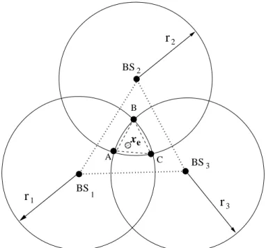
as in Fig. 8.1. It is noted that the three circles which define the TOA measurements will intersect to a single point (i.e. the MS’s position) if the measurements are LOS and are free of the measurement noises. The concept of the GLE algorithm is to consider the geometric constraints between the MS and the BSs within the formulation of the two-step LS method. It

(44)

0 0 1 1 BS BS BS A B C

r

_r

x_e 1 1 3 3 2 2

Figure 8.1: The Schematic Diagram of the TOA-based Location Estimation for NLOS envi-ronments (Generic Case)

is recognized that the range measurements are in general corrupted by both the measurement noises and the NLOS errors. The conventional two-step LS algorithm obtains location estimate primarily by considering the measurement noises with gentle NLOS errors. In the TOA-based location estimation as shown in Fig. 8.1, the location estimation by using the two-step LS method may fall around the boundaries of the three arcs, AB, BC, and CA, i.e. either inside or outside of these arcs. Since the overlap region (i.e. constrained by the points A, B, and

C) grows as the NLOS errors are increased, the location estimation of the MS acquired by

the two-step LS method will result in deficient accuracy (i.e. the location estimate still falls around the boundaries of the enlarged arcs AB, BC, and CA).

The primary objective of the proposed GLE algorithm is to confined the location estimate within the overlap region by including the geometric constraints into the two-step LS method. The following three different cases are considered based on the various cell layouts which may occur:

(45)

8.1.1 3 TOA Measurements – Generic Case

As illustrated in Fig. 8.1, three BSs associated with three TOA measurements are required for the location estimation of the MS. The overlap region (i.e. confined by the arcs AB, BC, and CA) is formed with the assumption that there is at least one NLOS error occurred from one of the three TOA range measurements. Since the objective of the proposed GLE scheme is to confine the estimated MS position within the region of ABC, the following constrained cost function is defined:

γ =   X µ=a,b,c 1 3kx − µk 2   1/2 (8.1)

where x is the MS’s location as mentioned before; a = (xa, ya), b = (xb, yb), and c = (xc, yc)

represent the corresponding coordinates of the points A, B, and C. γ is defined as a virtual

distance between the MS’s position and the three points A, B, and C. It is also noted that the

value of γ varies as the three coordinates a, b, and c are changed. An expected MS’s position

x_e is chosen to locate within the triangular area ABC in order to fulfill the constraints from

the geometric layout. The corresponding expected virtual distance γe can be obtained as

γe =   X µ=a,b,c 1 3kxe− µk 2   1/2 = γ + nγ (8.2)

where nγ is the error induced by the computed deviation between γe and γ. The major

functionality of the constrained cost function as in (8.2) is to minimize the deviation between

the virtual distance γ and the expected virtual distance γe. The selection of the expected MS

position xeis obtained by considering the signal variations from the three TOA measurements.

The coordinates of xe = (xe, ye) are chosen with different weights (w1, w2, w3) with respect

to the A, B, and C points of the triangle as

xe= w1xa+ w2xb+ w3xc (8.3a)

(46)

where w` = σ2 ` σ2 1 + σ22+ σ32 for ` = 1, 2, 3 (8.4)

σ₁, σ₂, and σ₃ are the corresponding standard deviations obtained from the three TOA

mea-surements, r1, r2, and r3. The decision of the weight w` is explained as follows. For the

measurement r1 (as shown in Fig. 8.1), the MS position should be located around the

bound-ary of the circle with the radius r1 without the existence of the NLOS errors. If the standard

deviation σ1 of the measurement r1 is comparably large, it indicates that the true position of

the MS should move toward inside of the circle boundary of the radius r1 due to the NLOS

errors. Consequently, the weight w1 is assigned with a larger value, which specifies that the

position of the MS should move toward the endpoint A of the triangle. The design concept is

applied to the selection of the other two weights, w₂ and w₃, in the same manner. With the

selection of the expected MS’s position xe, the expected virtual distance γe can be computed

from (8.2).

The proposed GLE algorithm is formulated by solving the two-step LS problem with the additional geometric constraint. The solution is obtained by minimizing both (i) the errors coming from the three TOA measurements (as in (2.1)) and (ii) the deviation between the

expected virtual distance and the virtual distance (as in (8.2)). By rearranging and combining

(2.1) and (8.2) in matrix format, the following equation can be obtained:

Hx = J + ψ (8.5) where x = · x y β ¸_T

(47)

H =          −2x1 −2y1 1 −2x2 −2y2 1 −2x3 −2y3 1 −2γx −2γy 1          J =          r₁2− κ1 r₂2− κ2 r2 3 − κ3 γ2 e− γκ         

The corresponding coefficients are given by

β = x2+ y2 κ` = x2` + y`2 for ` = 1, 2, 3 γx = 1₃(xa+ xb+ xc) γ_y = 1 3(ya+ yb+ yc) γκ = 1₃(x2a+ x2b + x2c+ y2a+ yb2+ yc2)

The noise matrix ψ in (8.5) can be obtained as

ψ = 2 c Bn + c2n2 (8.6) where B = diag ½ ζ1, ζ2, ζ3, γ ¾ n = · n1 n2 n3 nγ/c ¸_T

(48)

be obtained as

ˆ

x = (HTΨ−1H)−1HTΨ−1J (8.7)

where

Ψ = E[ψψT] = 4 c2 BQB

It is noted that Ψ is obtained by neglecting the second term of (8.6). The matrix Q can be acquired as Q = diag ½ σ2 1, σ22, σ23, σγe2 /c2 ¾

It can be observed that Q represents the covariance matrix for both the TOA measurements

and the expected virtual distance, where σ2

γe/c corresponds to the standard deviation of γe/c.

The final location estimation after the second step of the two-step LS algorithm can be obtained by referring the approach as stated in [25].

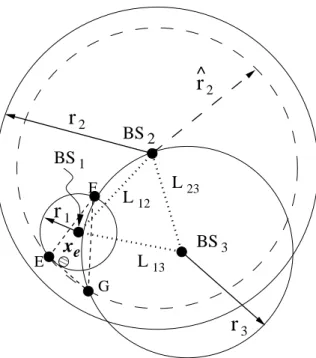
8.1.2 3 TOA Measurements – MS Locates Closer to its Home BS

In certain situations, the MS may locate much closer to its home BS compared to the other BSs. Due to the fact that the NLOS errors grow as the distance between the MS and the BS is increased [37], there is high possibility to result in no geometric intersection formed by these TOA measurements. As is illustrated in Fig. 8.2, there is no intersection between

the circles with the radiuses r1 and r2. Since the MS is located closer to its home BS (i.e.

BS₁), the non-intersect scenario occurs while there is larger NLOS error induced by the TOA

measurement from the BS₂. The original proposal as stated in the previous generic case will

not be applicable in this type of situation.

In order to employ the GLE algorithm within this circumstance, it is required to impose an

additional constraint to appropriately formulate the problem. The inequality of r` > L1`+ r1,

for ` = 2, 3, should be changed to ˆr` = L1`+ r1, where L1` corresponds the the distance

between the `th _{BS to the home BS. As shown in the Fig. 8.2, the modified radius ˆ}_r

2 results

(49)

0 0 1 1 BS BS 2 L L L₁₂ 23 13

r

E F G

^

x

_e 2 2 3 3 BS₁

r

₁

Figure 8.2: The Schematic Diagram of the TOA-based Location Estimation for NLOS envi-ronments (Special Case: MS Locates Closer to its Home BS)

proposed GLE scheme. It is noted that the assumption is applicable since the non-intersect situation is generally induced by the excessive amount of NLOS errors from the measurement

r2. As a result, the GLE algorithm can be applied in this case by substituting the points A.

B, and C (as in Fig. 8.1) with the points E, F , and G. Similar procedures can be employed

to solve for the two-step LS problem as mentioned in the previous case. The location estimate of the MS can therefore be constrained within the updated triangular area, which is enclosed by the points E, F , and G.

8.1.3 2 TOA and 1 AOA Measurements

Due to the weak incoming signals or the shortage of signal sources (e.g. at the rural area), there is great possibility that the MS may not be able to acquire enough signal sources from

the environment, i.e. only two TOA measurements are available from the BS1 and the BS2.

In order to employ the proposed GLE algorithm within this circumstance, an additional AOA measurement from the home BS is adopted. As mentioned in the 3GPP standard [33] [34], each BS should be equipped with the antenna arrays for adaptive beam steering in order to

(50)

0 0 1 1 θ

r

x_e I 2 AOA measurement K J

r

₁ BS₁ BS₂

Figure 8.3: The Schematic Diagram of the TOA/AOA-based Location Estimation for NLOS environments (Special Case: 2 TOA and 1 AOA Measurements)

facilitate the AOA measurements. It is also noted that only the AOA measurement from the home BS is applied to avoid the signal degradation due to the near-far effect. The geometric layout of the two TOA and the one AOA measurements is illustrated as in Fig. 8.3. The proposed GLE algorithm can be applied in this case with some modifications from the generic case. The region enclosed by the points A, B, and C (as in Fig. 8.1) is replaced by the

triangular area defined by the points I, J, and K. The selection of σ₃ within the expected

MS’s position (i.e. in (8.4)) should be modified as σ3 = r1· σθ/c, where σθ corresponds to the

standard deviation of the measurement noise n_θ as in (2.4). It is noted that σ3 is referred as

the signal variations coming from the AOA measurement. As the value of σ3 is increased, the

expected MS’s position xe should move away from the line which connects the points I and

J. The resulting location of xe is expected to move toward the point K as can be obtained

from (8.4).

In additions, the matrices, H and J, within (8.5) should be reformulated as

H =          −2x1 −2y1 1 −2x2 −2y2 1 − sin θ cos θ 0 −2γ_x −2γ_y 1         

(51)

J =          r2 1 − κ1 r2 2 − κ2 y1cos θ − x1sin θ γ_e2− γκ         

The matrices B, n, and Q associated with the noise matrix ψ as in (8.6) can be obtained as B = diag ½ ζ1, ζ2, ζ1, γ ¾ n = · n₁ n₂ n_θ n_γ/c ¸_T Q = diag ½ σ2 1, σ22, σ2θ, σ2γe/c2 ¾

It is noted that value in the third diagonal term within the matrix B, i.e. the element ζ1,

can be obtained as in [27] based on geometric approximation of the AOA measurement. The performance of the proposed GLE algorithm under the three different cases will be evaluated and compared via simulations in the next section.

8.2 The VBS Algorithm

In this section, the proposed VBS scheme is described in details. The observation from the GDOP effect is addressed in the chapter 8.3.1. Chapter 8.3.2 describes the concepts and motivations of the proposed VBS scheme; while the formulation of the algorithm is presented in the chapter 8.3.3.

8.2.1 Observation from the GDOP

The GDOP [36] is defined as the ratio between the location estimation error and the associated measurement errors. It is utilized as an index for observing the location precision of the MS under different geometric location within the network. In order to investigate the GDOP effect, a cell layout with three TOA measurements are considered as shown in Fig. 8.4.

(52)

0 0 1 1 BS BS BS 2 1 A B C r r 1 2 3 BS BS v v2 BS_v 1 x_e 3 r₃

Figure 8.4: The Schematic Diagram of the TOA-based Location Estimation with the Virtual Base Stations 0 500 1000 1500 2000 0 500 1000 1500 0.5 1 1.5 2 Y(m) X(m) GDOP 0 500 1000 1500 2000 0 500 1000 1500 0.5 1 1.5 2 Y(m) X(m) GDOP

Figure 8.5: Left Plot: GDOP Contours using Three TOA Measurements; Right Plot: GDOP Contours with One Virtual BS inside the Triangular Area

(53)

0 500 1000 1500 2000 0 500 1000 1500 0.5 1 1.5 2 Y(m) X(m) GDOP 0 500 1000 1500 2000 0 500 1000 1500 0.5 1 1.5 2 Y(m) X(m) GDOP

Figure 8.6: Left Plot: GDOP Contours with One Virtual BS outside the Triangular Area; Right Plot: GDOP Contours with Three Virtual BSs outside the Triangular area

The three BSs are assumed to locate at the coordinates (0, 0), (1000, 1000√3), and (2000,

0) in meters. The locations of the MS are designed to be within the enclosed triangular area

formed by the three base stations. i.e. points BS1, BS2, and BS3. The left plot of Fig. 8.5

shows the GDOP effect for the three TOA measurements within the triangular region. It can be seen that there is worse GDOP effect (i.e. with higher GDOP values) around the areas close to the three BSs comparing with the other region within the triangular area. In order to further observe the GDOP effect, it is possibility to provide an additional BS with adjustable location within the network. The right plot of Fig. 8.5 illustrates the GDOP effect with the

4th _{BS located at the center of the triangle BS}

1BS2BS3; while the left plot of Fig. 8.6 shows

that with the 4th _{BS situated outside of the triangular area, i.e. at point BS}

v2 as in Fig.

8.4. It can be observed form the right plot of Fig. 8.5 that not much GDOP improvement

is achieved by placing the 4th _{BS within the triangular region. On the other hand, it is}

interesting to find that the high GDOP value around the BS₁ and BS₃ can be reduced by the

4th_{BS situated outside of the triangular area (as in the left plot of Fig. 8.6). Moreover, it can}

be seen from the right plot of Fig. 8.6 that the comparably worse GDOP values around the

行動設備之無線定位技術

Wireless Location Estimation and Tracking System for Mobile

Devices

Contents

Chapter 1

Introduction

Chapter 2

Related Work

2.1

Mathematical Modeling

2.2

Sources of Ranging Errors

BS

2.3

Studies on Existing Location Estimation Algorithms

Part I

Hybrid Location Estimation and

Tracking System for Mobile Devices

Chapter 3

Overview

Chapter 4

System Architecture

Chapter 5

The Location Estimation and

Tracking Algorithms

5.1

Two-Step Least Square Location Algorithm

5.2

Kalman Filtering

5.3

Data Fusion

Chapter 6

Performance Evaluation

6.1

The Noise Model

6.2

Simulation Parameters

6.3

Simulation Results

Part II

Enhanced Wireless Location

Estimation Algorithms

Chapter 7

Overview

Chapter 8

The Proposed GLE and VBS

Algorithms

8.1

The GLE Algorithm

r

r

r

r

r

r

^

x

r

r

r

8.2

The VBS Algorithm

_r