解碼端影像誤差估測用於分散式視訊編碼法校正優先權的設計

國

立

交

通

大

學

多媒體工程研究所

碩

碩

碩

碩

士

士

士

士

論

論

論

論

文

文

文

文

解碼端影像誤差估測用於分散式視訊編碼

法校正優先權的設計

Adaptive Decoder Side Information Error Estimation for

Priority-based Error Correcting Distributed Video Coding

研 究 生：連曉玉

指導教授：蔡淳仁 教授

中

中

中

中 華

華

華

華 民

民

民

民 國

國

國

國

九

九

九

九 十

十 八

十

十

八

八

八

年

年

年

年 二

二

二

二 月

月

月

月

解碼端影像誤差估測用於分散式視訊編碼法校正優先權的設

計

Adaptive Decoder Side Information Error Estimation for

Priority-based Error Correcting Distributed Video Coding

研 究 生：連曉玉 Student：Shiau-Yu Lian

指導教授：蔡淳仁 Advisor：Chun-Jen Tsai

國 立 交 通 大 學

多 媒 體 工 程 研 究 所

碩 士 論 文

Submitted to Institute of MultimediaEngineering College of Computer Science

National Chiao Tung University in partial Fulfillment of the Requirements

for the Degree of Master

in

Computer Science February 2009

Hsinchu, Taiwan, Republic of China

解碼端影像誤差估測用於分散式視訊編碼法校正優先

權的設計

摘要

摘要

摘要

摘要

分類的資訊經由一個上傳 channel 傳回編碼端，所以誤差程度相似的 macro-block 會被聚集在一起以進行 channel coding。使用這種方法，解碼端可 以為 side information 品質比較不好的 macro-block 要求多一點的 parity bits 以更正這些部分的錯誤。而對於 side information 誤差較小的 macro-block 則 要求比較少的 parity bits。比起目前最好的 DISCOVER DVC codec，對於 QCIF sequences，在較低的 bitrate 範圍裡(低於 200 kbps)我們所提出的 DVC 架構可

以使 R-D performance 增加 0.3 至 0.5 dB。因為低複雜度的編碼器對於像是 sensor network 之類的低 bitrate 監視應用系統是很重要的，所以我們所提出

Adaptive Decoder Side Information Error Estimation

for Priority-based Error Correcting Distributed

Video Coding

Student: Shiau-Yu Lian Advisor: Dr. Chun-Jen Tsai

Institute of Multimedia Engineering National Chiao Tung University

Abstract

In this thesis, a distributed video coding technique with prioritized channel coding of W-Z frames is presented. In the proposed framework, W-Z frame

macro-blocks are classified into different groups based on the estimated errors of the side information. The information is transmitted via uplink channel back to the encoder so that macroblocks with similar error statistics can be grouped tighter in same coding blocks for channel coding. With this approach, decoder can request more parity bits to correct macroblocks whose side information quality is worse and request less or no parity bits for macroblocks with small side information errors. The

proposed DVC scheme can increase R-D performance about 0.3 to 0.5 dB over the state-of-the-art DISCOVER DVC codec for low bitrate (less than 200 kbps)

applications for QCIF sequences. Since low-complexity encoder is important for low bitrate surveillance applications such as those for sensor networks, the proposed scheme is very promising for practical applications.

謝誌

謝誌

謝誌

謝誌

Table of Contents

摘要... I

Abstract ... III

謝誌... V

Table of Contents ... VI List of Figures ... VII List of Tables ... IX

Chapter 1: Introduction ... 1

Chapter 2: Previous Work ... 4

2.1 Stanford’s DVC Frameworks ... 6

2.2 Side Information Generation... 8

2.2.1 Interpolation and Symmetric Motion Model ... 9

2.2.2 Hash Information as Motion Cue ... 11

2.3 Channel Coding for Side Information Correction ... 13

2.3.1 Virtual Channel Model ... 13

2.3.2 Channel Code ... 15

Chapter 3: Analysis on DVC Virtual Channel Error Characteristics ... 17

3.1 Study on Virtual Channel Models ... 17

3.1.1 Types of Channel Models ... 17

3.1.2 Adaptive Laplace Channel Model for Each Bit-planes ... 22

3.2 LDPCA Decoding ... 24

3.2.1 LLR (Log Likely-hood Ratio) Values ... 24

3.2.2 Over-Corrected Pixels ... 28

3.2.3 Prioritized Decoding of Side Information Pixels ... 31

Chapter 4: System Architecture ... 32

4.1 System Block Diagram ... 32

4.2 Side Information Generation... 34

4.3 Macroblock Classification and Grouping ... 37

4.4 Transform and Quantize ... 42

4.5 LDPCA Encoding ... 45

4.6 LDPCA Decoding and Reconstruction ... 45

4.7 Pixel Domain DVC Codec ... 48

Chapter 5: Experimental Results ... 50

List of Figures

Figure 1. Performance of the cue-based DVC scheme in [22] ... 6

Figure 2. R-D performance of the DVC scheme in [18] ... 11

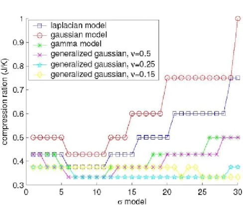
Figure 3. Compression ratio when different error models are used ... 14

Figure 4. Decoding graph of LDPC codes and LDPCA codes ... 16

Figure 5. Rate required by turbo codes and SLDPCA codes ... 16

Figure 6. Histograms of Laplace parameters (mean and scale) ... 19

Figure 7. R-D curve of ‘Foreman’ and ‘Mother and Daughter’ ... 21

Figure 8. Error distributions when 1st ~ 4th bit-planes are decoded ... 23

Figure 9. R-D curve of ‘Foreman’ when different Laplace models are used for each bit-plane 24 Figure 10. P(x = 0) and corresponding LLR values ... 25

Figure 11. Absolute values of LLR when decoding 1st bit-plane of ‘Foreman’ 2nd frame ₂₅ Figure 12. Absolute value of LLR and pixel value of side information when decoding 1st bit-plane of ‘Foreman’ 2nd _{frame ... 26}

Figure 13. Absolute value of LLR and pixel value of side information when decoding 2nd bit-plane of ‘Foreman’ 2nd _{frame ... 27}

Figure 14. Absolute value of LLR and pixel value of side information when decoding 2nd bit-plane of ‘Foreman’ 2nd _{frame ... 27}

Figure 15. R-D performance when ignoring pixels with side information near ‘crossing threshold’ and small residual ... 30

Figure 16. R-D performance when decoder ignore pixels with side information values near ‘crossing threshold’ ... 30

Figure 17. System flow of our transform domain DVC codec ... 33

Figure 18. Motion estimation for neighboring key frames ... 34

Figure 19. Bi-directional motion adjustment ... 34

Figure 20. Macroblock rearrange ... 39

Figure 21. R-D performance when different cues are used by the decoder to pick up worse macroblocks... 42

Figure 22. Quantization matrices ... 43

Figure 23. The relationship between AC coefficients and quantized values ... 45

Figure 24. Probability calculation of second significant bit when most significant bit is decoded as 1 ... 46

Figure 25. Side information is reconstructed to the stripe pattern area when the decoded value is 0 ... 47

List of Tables

Table 1. PSNR of side information using different prediction tools ... 20

Table 2. Percentage of over-corrected pixels and under-corrected pixels of foreman 2nd _{frame ... 28}

Table 3. QP Values for encoding key frames ... 43

Table 4. DISCOVER DVC codec testing setting ... 51

Chapter 1: Introduction

Distributed video coding (DVC) is a new video coding paradigm which allows more flexible coding complexity distribution between encoder and decoder. Traditional video codecs, for example, H.264, is designed for the situation where video is encoded once and decoded many times. The coding efficiency is mainly determined by the computational power of the encoder. But now there are many new applications, such as sensor networks and security camera systems, where the computational power of the encoder (sensors or cameras) is weaker than the decoder (central receiver of recorded videos). For these applications, a reversed paradigm is needed, and distributed video coding is suitable for this situation.

In traditional closed-loop video coding systems, motion estimation at the encoder side is used to eliminate temporal correlation of video data and the information of correlation is transmitted to decoders as motion vectors. The main idea of DVC is to estimate-and-construct the inter-frame correlation at the decoder side with little help from the encoder; therefore, the computation burden of motion estimation is shifted to the decoder [1]. For a typical DVC system, the video source would be divided into two interleaving sub-sequences: key frame subsequences and Wyner-Ziv (W-Z) frame subsequences. Key frames would be encoded using traditional encoder (such as the motion JPEG encoder or any video encoder).

For W-Z frames, the encoder takes the original video frame as input and applies a low-complexity algorithm to predict and generate some data (refer to as W-Z bits) that can help the decoder correct any errors in generation of the target frames (refer to as the side information). On the decoder side, the side information (SI) would be generated first using any information reconstruction technologies based on temporal correlation of neighboring key frames. And then, a W-Z decoder uses the W-Z bits

from the encoder to correct any potential errors in the SI such that the resulting W-Z frames would be close to the original frames at the encoder side. The key components in a DVC framework are the W-Z bits generator and the SI generator.

The main complexity of encoder in traditional video codec architecture is due to motion estimation. For distributed video coding, we want a simple, low power encoder and a powerful decoder. So the encoder cannot perform motion estimation anymore; the job of predictive coding should be shifted to the decoder side. Whether this new paradigm can achieve the same coding performance as traditional video codec is an important research topic. According to previous information theory research results, the compression efficiency of distributed video coding should match that of traditional video coding techniques. Two of the most fundamental results related to the concept of distributed video coding from information theory are Slepian-Wolf theorem [2] and Wyner-Ziv theorem [3]. The latter is a lossy version of the former theorem.

Consider when we want to encode two statistically dependent variables, X and Y. According to information theory, fewer bits (H(X, Y)) are needed to describe the two variables if we jointly encode them. For video coding, two successive frames can be coded more efficiently if we consider their predictable relationship by motion estimation, and then encode the unpredictable residuals. But if the two variables X and Y are separately encoded, how many bits are required to describe them? For video coding, what bitrate will be required if frames are intra coded instead of inter coded?

The Slepian-Wolf theorem tell us that even if two variables X and Y are separately encoded, once they are jointly decoded, only H(X, Y) bits are required to decode them. For video coding, when frames are intra coded, if the decoder can jointly decoded them, the same coding efficiency can be reached. So, theoretically, in distributed

video coding, if the decoder can jointly decode frames, that is, the decoder know the relationship between the frames and use the information to decode the frames, then only H(X, Y) bits will be sent to the decoder even if the encoder encodes the frames in intra mode. The theorem tells us that the performance of distributed video coding should as good as that of traditional video coding in theory. But until today, there is no technique based on distributed video coding principle whose performance can be close to that of traditional video coding.

In this thesis, a macroblock rearranging method is proposed to enhance R-D performance of distributed video coding. Existing distributed video coding methods performs particularly worse at low bit-rate end of the R-D curve. For QCIF sequence with frame rate 15 Hz, the proposed techniques can improve the performance of existing method by about 0.5 dB in PSNR measure when bit-rate below 200 kbps. This bit-rate range is reasonable for QCIF sequence. The proposed technique uses some cues to detect at the decoder side which part of the predicted side information has potentially high prediction errors and provide the encoder with this information. The encoder then rearranges the macroblocks so that the channel code-based W-Z bits generation process can be more efficient. As a result, the decoder can request W-Z bits to correct the hard-to-predict macroblocks first. Experimental results show that this technique outperforms current distributed video coding techniques, particularly at low bit-rate ends.

The organization of this thesis is as follows. Chapter 2 presents a literature survey on previous work of distributed video coding. In chapter 3, some analyses are conducted to identify the weakness of current techniques. In chapter 4, the proposed block rearranging method and system architecture will be described. And the experimental results will be presented in chapter 5. Finally discussions and future work are given in chapter 6.

Chapter 2: Previous Work

The key components of distributed video coding are generation of side information (predicted target frame at the decoder, using only key frames as the hypotheses) and coding of W-Z bits (data used to correct prediction error at the decoder side). Currently, there are two major approaches on side information generation: projection-based motion compensation and cue-based motion compensation. The first method performs moving block trajectory projection based on motion smoothness assumption. The projection-based compensation has several variations such as multi-frame reference projection [20] or sub-pixel motion projection [5].

An alternative approach on SI generation is the cue-based motion estimation scheme. In this method, the encoder sends not only W-Z correction bits but also some image cues for side information generation. The decoder can thus do more accurate inter-frame correlation discovery using cue bits. Several techniques have been proposed for cue generating functions, such as CRC codes [6], high pass filters in the DCT domain [40], and low pass filters in the DCT domain [13]. Although projection-based methods do not require the encoder to send extra cue bits, comparing to cue-based estimation, projection-based methods only performs well with ideal motion behavior. On the other hand, cue-based estimation could provide more robust and accurate side information but consumes extra bandwidth.

As in traditional close-loop codecs, it is not efficient to use only one coding tool to handle coding of all video signals. For DVC, the motion projection-based tool and the cue-based tool are suitable for constructing SI for different types of video signals. Therefore, low-complexity mode decision at the encoder side is crucial for improving the performance of DVC codecs. Some DVC frameworks use the differences of

co-located blocks to distinguish the background from the foreground and to determine the cue bits [13]; however, this approach is limited to stable background patterns.

Kang and Lu proposed a wavelet-based DVC framework [26]. They use Structural Digital Signature (SDS) [30] to determine which wavelet coefficients are important, and only these coefficients are sent. For a wavelet tree structure, SDS records magnitude relation of every node and its child node. If the SDS of wavelet coefficients is different between two frames, then the two frames are perceptually different.

SDS of each frame are calculated and compared with the previous frame. Wavelet coefficients with SDS different from their co-located blocks in previous frame are marked as important coefficients. Only important coefficients are sent to the decoder. For non-important coefficients, the decoder copies coefficients from previous frame. If there are too many important coefficients, then H.264 intra coder will be used instead. This is a framework that both the complexity of the encoder and the decoder are low at the same time.

Figure 1 is the RD performance of this method. The plot above in this figure is R-D curve of Hall sequence, and the plot below is R-D curve of Foreman sequence. Most part of the Hall sequence is the background without motion, so the number of important coefficients is small. The performance is near other DVC methods, but comparing to a traditional video codec such as H.264, there is still a gap. For the Foreman sequence, most part of the frames is composed of the moving face, the PSNR of current frame and previous frame is small, so the number of important coefficients is large. Most blocks are coded using H.264 intra coder, so the performance is near the H.264 intra case. We can see, this method is only suitable for sequences with little foreground moving objects, such as in some security camera applications.

Figure 1.Performance of the cue-based DVC scheme in [22]

2.1 Stanford’s DVC Frameworks

One of the most adopted DVC framework is proposed by Aaron et al. [1][7][8][11][12][13][14]. In this work, the encoder consists of a quantizer, a channel encoder, a buffer, and a traditional intra encoder. The decoder consists of a channel decoder, a side information generator, a frame reconstructor, and a traditional intra decoder.

At the encoder side, frames in a video sequence are first divided into even frames and odd frames. The odd frames are intra coded using traditional video codec such as H.264, and these frames are called ‘key frames.’ The even frames are like B-frames in

traditional video codecs, and these frames are called ‘W-Z frames.’ But in DVC the encoder does not perform motion estimation and encode the residual. Instead, it treats these W-Z frames like I frames and encodes them independently by a channel encoder. The systematic channel encoder produces systematic message bits (the original pixel values) and parity bits (refer to as the W-Z bits), but only W-Z bits are stored in the buffer. The systematic bits are all discarded.

At the decoder side, for the ‘key frames,’ the decoder use traditional intra decoder to decode them. For the ‘W-Z frames,’ the decoder use key frames neighboring the W-Z frame to generate “side information” of this W-Z frame. The side information is like predictor in traditional video codec but is only known by the decoder. The decoder can use any information it has to generate (predict) side information. For example, the key frames already received can be used as the motion compensation hypotheses.

After generating the side information, the decoder needs additional bits for correcting the errors in the side information and reconstructing the original frames. This is like receiving residuals from encoder in traditional video codec. But the encoder does not know side information; it only generates W-Z bits of frame. The decoder requests for W-Z bits and use channel decoder to decode frames. The systematic bits are discarded at encoder side, so the decoder uses side information as the systematic bits. By the theory of channel coding, if the channel condition is good (that is, the decoder prediction error is small), the cross probability is small, and then fewer bits are needed for recovering the original signal. To be more specific, for DVC, if the side information of the target frame predicted by the decoder is almost the same as the W-Z frame we want to decode, then fewer W-Z bits are requested, coding efficiency is better.

DCT domain, and spatial redundancy within a frame is not explored. In [14], DCT domain coding is added to the framework because the performance is better.

In traditional video codecs, when GOP size increases, the coding efficiency will increase too. That is because there will be more P frames and B frames. In the first version of the Stanford DVC framework, GOP size is 2. That is, for every two frames, there is only one W-Z frame. Aaron et al. [11] try to use larger GOP size but the performance decreases as the GOP size increases. This is very different from traditional video codec. This is because when GOP size increases, the distance between W-Z frame and available key frames used to generate side information also increases, hence, the quality of the side information decreases.

To further improve the coding efficiency, Brites er al. from the DISCOVER DVC team [16] proposed a variable step size quantization which can make DCT coefficients less distorted when the dynamic range of coefficient band is smaller. That is, for a fixed number of quantization levels, if we know the dynamic range, then a sufficient and small step size can be used, and the distortion can be smaller. But additional bits are required for representing the value of dynamic range. This method may be inspired from H.264.

2.2 Side Information Generation

Side information quality directly affects coding efficiency in a DVC codec, therefore, a lot of research efforts in DVC are devoted to side information generation algorithms. In [17], some experiments are conducted to show the relation between PSNR of side information (compared with the original W-Z frame), and number of W-Z bits requested. In summary, when PSNR of side information is higher, fewer W-Z bits are needed and the compression ratio is higher.

2.2.1 Interpolation and Symmetric Motion Model

Side information can be interpolated or extrapolated from key frames and previously reconstructed WZ-frames. This is similar to motion-compensated frame interpolation which is used to increase frame rate at decoder side. There are many models being proposed for motion-compensated interpolation. For example, Liu et al. [29] assume that every frame has same motion field. This model of course is too simple so that the side information generated are not good. The symmetric motion model is a simple model but its performance is acceptable for some cases. Many researchers adopt symmetric motion model and use processing to enhance its performance [7][18].

The algorithm of the symmetric motion model is explained as follows. If the W-Z frame is frame Y, and its previous key frame is frame X, next key frame is frame Z. Symmetric motion model assumes that the object moves at a constant speed. So if the position of object O is (x1, y1) in frame X and (x1+mvx, y1+mvy) in frame Z, then

the position of object O should be (x1+mvx/2, y1+mvy/2). When the decoder wants to

generate side information of frame Y, it has already received frame X and Z. So it can perform traditional motion estimation on frame X and Z. For macroblock M at (x1, y1)

in frame Z, there is a best matched macroblock N at (x1+mvx, y1+mvy) in frame X.

Then the decoder will project the average of M and N to (x1+mvx/2, y1+mvy/2) onto

frame Y along the motion path of M and N.

Of course there are many problems when using this model to implement side information generator. First of all, there may be some macroblocks which do not satisfy this single-object constant motion model. A macroblock may contain two or more objects, or objects which do not move at a constant speed. Secondly, when the decoder projects every matched macroblock pair to W-Z frame, there may be some

pixels which have no projection, or twice or more projections. For pixels that are projected twice or more, it is not trivial to choose the best projection pair without knowledge of the original W-Z frame. For pixels that have no projections, the decoder must use some algorithms to interpolate their values as well.

Klomp et al. [5] believe that using motion estimation with more accuracy may increase side information quality. However, due to motion model mismatch, the actual improvements could be very little. Li and Delp [20] conducted some experiments on the amount of macroblocks in key frames used to generate side information. They discovered that the more macroblocks used, the better side information is generated, especially when these macroblocks come from different key frames.

In the above two proposals, decoders must do more computations to either increase motion estimation accuracy or to increase the number of reference macroblocks used. Ascenso et al. in DISCOVER team [18] adopt a different approach and develop a pixel domain DVC codec IST-PDWZ and a transform domain DVC codec IST-TDWZ. Their proposed technique is also based on the framework from Stanford with symmetric motion model. But before performing motion estimation on key frames, a low pass filter is used to make the estimated motion vectors less noisy. After obtaining motion vectors, if macroblock Y would be the average of macroblock X and Z. Bi-directional motion estimation is then used to fine-tune the motion vectors. After that, a smoothing filter is applied to the motion vectors because the motion field should be smooth. We can see the R-D performance in 0, this adjustment indeed makes performance better.

Figure 2.R-D performance of the DVC scheme in [18]

2.2.2 Hash Information as Motion Cue

In previous section we see how to use symmetric motion model to utilize key frames to generate good side information. We know symmetric motion model is limited. To further increase the quality of side information, it is possible for the encoder to compute and transmit some extra information to assist the decoder to generate better side information. Some researchers refer to this information as hash [13]. When decoder wants to generate side information, it does not perform motion estimation on neighboring key frames. Instead, it can obtain motion vector by directly comparing hashes of macroblocks. When hashes of two macroblocks are similar, the content of these two macroblocks are expected to be similar too.

Traditional hashes, for example, CRC and MD5, are very sensitive to content changing. But hashes used to compare image similarity should only be sensitive to perceptual changes in the pixel data. This kind of hash is called media hash, robust hash, soft hash, and image fingerprinting. Distance between hashes can be used as a measure of content similarity. If the hash is good enough, that is, a decent

representation of macroblocks, motion estimation by comparing hash shall give us a good result.

Media hash design is an active research topic, and many papers have already been published. But most of these papers design media hash for content-based retrieval, watermarking, image authentication, and image database management. Media hash can be implemented by calculating the histogram of image [34], or the position of edges [35] or feature points [36]. DCT sign information is also useful [37]. The researchers hope that the media hash can be robust to geometric transformation and compression. So calculations of some media hashes are sometimes too complicated, and they are not suitable for DVC. Furthermore, these applications do not concern about the size of hashes, but for DVC, hash size affects bitrate.

For DVC, simple and small hashes are considered. In [13], using hash to help decoder to generate side information is first mentioned. The authors use sub-sampled and coarsely quantized version of macroblock in W-Z frame as their hash. To decrease overhead of hash, when co-located macroblock in previous key frame is similar to macroblock in current W-Z frame, no-hash bit is sent instead.

Girod et al. [8] also mentioned that the possibility of using high frequency portion of a macroblock as a distinct feature of the block. For an 8-by-8 block, 54 most high frequency coefficients (most of them may be zeros) with run-length and Huffman compression are sent to decoder as hashes. The remaining 10 low frequency coefficients are channel encoded and decoded. Although this idea seems reasonable, but in practice, it is not trivial for decoder to perform motion estimation based on high frequency coefficients.

2.3 Channel Coding for Side Information Correction

The key concept in DVC is that the side information predicted at the decoder side can be regarded as a video frame corrupted during the transmission over a (hypothetical) noisy channel. In DVC, the communication channel between the encoder and the decoder is a virtual noisy channel and side information is the noisy version of the original frame transmitted from the encoder across the channel to the decoder. Since the encoder has knowledge of the original frames, it can generate systematic channel codes to correct any potential errors of the side information at the decoder side. In practice, only the W-Z bits of the channel codes have to be transmitted to the decoder. There are many factors of channel coding that affect the coding efficiency of the DVC framework. Two of the most significant factors are the model of the virtual noisy channel and the channel code used.

2.3.1 Virtual Channel Model

For channel decoding, fewer W-Z bits will be requested if we know more about the nosie characteristics of the channel. But in DVC the noise is strongly related to side information quality which is not stationary. In early days, only one single statistics model (usually Laplace distribution), is used to describe the noise distribution for the whole sequence or the whole frame. This is not practical, because actual noise distribution is far more complicated and cannot be modeled by a single Laplace distribution. Borchert et al. [21] propose that if each frame is partitioned into two types of regions, occluded regions and non-occluded regions, and two different statistics models are used to model the errors for different types of regions, the performance will be better than using one statistics model for the whole frame.

parameters of the error distribution. The decoder need to estimate the parameters. However, one may not need exact parameters since the decoding algorithm allows some tolerance on the exactness of the statistics model. The tolerance range of the parameters is different from frame to frame. A distribution which is not sensitive to errors in parameter estimates and achieves high compression ratio such that decoder only needs few W-Z bits from the encoder to correct SI prediction errors is desired. Westerlaken et al. [22] have shown that when a single distribution is used to describe channel noise, two-sided Gamma and generalized Gaussian distribution have better decoding performance than Laplace and Gaussian distributions when LDPC codes are used. The compression ratio when using different error models is in Figure 3. They also discovered that for generalized Gaussian, there is a small range of shape parameter that makes LDPC performance less sensitive to the choice of the variance parameter. But they do not mention how to find this small range.

2.3.2 Channel Code

In DVC, the virtual channel noise is not stationary, so rate-adaptive channel codes are needed in distributed video coding schemes. Channel codes near theoretical bound and rate-adaptive are suitable for DVC. Punctured turbo codes are well known for their burst error correcting capability and their performance is very close to Slepian-Wolf bound [23], so at the beginning, many DVC papers use turbo codes as their channel codes.

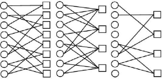
Low Density Parity Check (LDPC) codes are also channel codes near Slepian-Wolf bound. They have been used effectively in fixed-rate distributed source coding [25]. But in rate-adaptive cases, syndromes are punctured before they are sent, when compression ratio is high, the performance will be poor because in the decoding graph there are many single-connected or isolated nodes. The Stanford team presents two kinds of LDPC-based rate-adaptive codes: LDPC Accumulate codes (LDPCA) and Sum LDPC Accumulate codes (SLDPCA) [15]. The syndrome bits of LDPCA and SLDPCA codes contain more redundant information because of accumulation, so when a subset of syndrome bits are truncated, the performance will not be affected as much as the original LDPC codes. In Figure 4, circles are source bits and squares are parity bits after encoding. Left picture is the decoding graph of LDPCA code when all parity bits are not discarded. The center picture is the decoding graph of LDPCA code and the right picture is decoding graph of LDPC when half of parity bits are discarded. All nodes in the LDPCA decoding graph are neither isolated nor single-connected, so when compression ratio is high, LDPCA codes still have good performance.

Figure 4.Decoding graph of LDPC codes and LDPCA codes

Figure 5.Rate required by turbo codes and SLDPCA codes

In 0, we can see that when conditional entropy H(X|Y) is larger than 0.5, the rate required for turbo codes increases faster and becomes bigger than LDPC codes, especially when H(X|Y) is larger than 0.8. Furthermore, LDPCA has one advantage over turbo codes, that is, syndrome bits can be used to test the correctness after decoding. When the error position can be detected after decoding, we can do something to enhance the regions where errors are serious. In [28], the authors decode the first 3 bit-planes and then perform full searches for side information which significantly reduces decoding errors. After adjusting the side information, the decoder keeps decoding remaining bit-planes, and the performance is better.

Chapter 3: Analysis on DVC Virtual Channel

Error Characteristics

In this chapter, we have conducted some investigations on the performance of DVC-based coding mechanisms. In addition to examine the impact of error distribution models on coding efficiency, we also study the validity of the common DVC assumption of using log likelihood ratio as an indication of the reliability of the side information values. All experiments we describe here are tested using our pixel-domain DVC framework with lossless key frames. The frame rate is 30 fps.

3.1 Study on Virtual Channel Models

3.1.1 Types of Channel Models

In DVC coding schemes, a Laplace distribution L (µ, b) is in general used to model the prediction error of side information. The parameter µ is the mean parameter and often set to 0. The parameter b is the scale parameter. So, the probability density function of errors is f x =be−bx−µ

2 )

( . This definition is often adopted in DVC papers, which is slightly different from the traditional Laplacian probability density function

b x e b x f µ − − = 2 1 )

( . We use the definition former, so when the errors are more concentrated, the value of scale parameter will be larger. The two parameters may be estimated using some sample video sequences offline or estimated by the decoder adaptively while decoding a sequence. However, our initial experiments show that when a single distribution model with few parameters is used, the coding efficiency of the DVC schemes is relatively insensitive to the distribution being used to model the “channel-imposed” error of side information. In other words, correctly choosing parameters of distribution does not affect number of LDPC correction bits very much.

The reason is that the side-information prediction error model is quite different from the communication channel error model. In side-information prediction, large errors may also occur when energy of original signals are high due to errors in motion compensation models. That is, even when pixel values in original frames are big, it is still possible that the side-information errors are serious.

In order to test the relation between the accuracy of channel error model parameters and the error-correction efficiency on the prediction errors of the side information, we use three different distributions: Laplace, Gaussian, and uniform distributions to model channel errors. The parameters of Laplace distribution and Gaussian distribution are calculated offline. The uniform distribution is used to simulate the situation where we do not know error distributions at all.

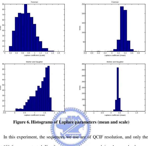
In addition, an adaptive channel error model is also used in which, the distribution parameters are estimated not for the whole sequence, but adaptively for every 44×48 region of pixels. Therefore, the adaptive error model should fit the true error distribution mush better than the non-adaptive ones. The histograms of the estimated Laplace parameters of the side-information prediction error models for the ‘Foreman’ and the ‘Mother-and-Daughter’ sequences are shown in Figure 6. One can see that when the ‘scale’ parameter of Laplace distribution is larger, the error distribution is more concentrated around the mean. Many areas in the ‘Mother-and-Daughter’ sequence have very small residuals, so when using a Laplace model to fit it, the scale parameters are larger than that of the ‘Foreman’ sequence.

-0.80 -0.6 -0.4 -0.2 0 0.2 0.4 0.6 0.8 1 50 100 150 200 250

Laplace coefficient (mean)

ti m e s Foreman -1.50 -1 -0.5 0 0.5 1 1.5 2 50 100 150 200 250 300 350 400

Laplace coefficient (mean)

ti

m

e

s

Mother and Daughter

Figure 6.Histograms of Laplace parameters (mean and scale)

In this experiment, the sequences we use are of QCIF resolution, and only the first 101 frames are tested. Key frames are not compressed, in other words, they are lossless. The motion compensated interpolation procedure similar to that proposed in IST-PDWZ [38] with key frame smoothing and fine-tuning of bi-directional motion vectors is used to increase side information quality. The side information PSNR values using different tool combinations are listed in Table 1. Based on Table 1, tool set (d) is used in the following experiments. We calculate the R-D curves for W-Z frames and see how channel noise model chosen affects coding performance of side information prediction errors.

0 0.2 0.4 0.6 0.8 1 1.2 1.4 1.6 1.8 2 0 10 20 30 40 50 60 70 80 90

Laplace coefficient (scale)

ti m e s Foreman -0.50 0 0.5 1 1.5 2 2.5 10 20 30 40 50 60 70 80 90

Laplace coefficient (scale)

ti

m

e

s

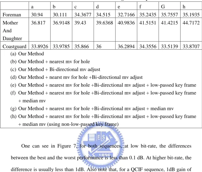
Table 1. PSNR of side information using different prediction tools a b c d e f G h Foreman 30.94 30.111 34.3677 34.515 32.7166 35.2435 35.7557 35.1935 Mother And Daughter 36.817 36.9148 39.43 39.6368 40.9836 41.5151 41.4215 44.7172 Coastguard 33.8926 33.9785 35.866 36 36.2894 34.3556 33.5139 33.8707 (a) Our Method

(b) Our Method + nearest mv for hole (c) Our Method + Bi-directional mv adjust

(d) Our Method + nearst mv for hole +Bi-directional mv adjust

(e) Our Method + nearest mv for hole +Bi-directional mv adjust + low-passed key frame (f) Our Method + nearest mv for hole +Bi-directional mv adjust + low-passed key frame

+ median mv

(g) Our Method + nearest mv for hole +Bi-directional mv adjust + median mv

(h) Our Method + nearest mv for hole +Bi-directional mv adjust + low-passed key frame + median mv (using non-low-passed key frame)

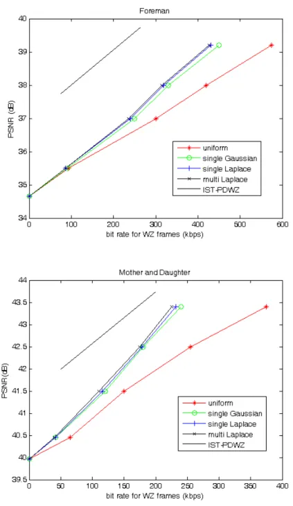
One can see in Figure 7, for both sequences, at low bit-rate, the differences between the best and the worst performance is less than 0.1 dB. At higher bit-rate, the difference is usually less than 1dB. Also note that, for a QCIF sequence, 1dB gain of PSNR above 40dB is virtually not perceptible by human observer under normal viewing conditions. It means that for most significant bit-plane, choosing Laplace or Gaussian model dose not affect performance much in practical sense.

Figure 7.R-D curve of ‘Foreman’ and ‘Mother and Daughter’

The results from IST-PDWZ are also projected in Figure 7. Although the final PSNR of our corrected side information is worse than those published in [38] for about 2.5 dB, the slopes of our R-D curves are the same or even larger than the slopes of the curves of IST-PDWZ. The difference in PSNR is largely due to the initial quality of side information before error correction. The differences in slopes may be due to different channel coding techniques (LDPCA in our experiments, and turbo

-1500 -100 -50 0 50 100 150 0.05 0.1 0.15 0.2 0.25 Residual of SI P ro b . Foreman Residual Range: [-132 109] -80 -60 -40 -20 0 20 40 60 80 0 0.05 0.1 0.15 0.2 0.25 0.3 0.35

Residual of SI after 2nd bitplane decoded

P ro b . Foreman Residual Range: [-63 63]

coder in IST-PDWZ) and it shows that the channel coding efficiency of LDPCA may be better than that of turbo code for DVC.

3.1.2 Adaptive Laplace Channel Model for Each Bit-planes

In previous section we see that the channel behavior-based error model only has marginal influence on DVC coding efficiency. One of the possible reasons is due to the fact that side information errors are not spatially invariant. Therefore, single error channel model is not sufficient for modeling the entire sequence. But in previous graph, we can see that even by choosing different parameters for each small area adaptively, the performance increase is not obviously. Other possible reasons are that single error model is used for every bit-plane decoding, or that the channel decoding method used in many DVC papers is not suitable for DVC.

-1000 -80 -60 -40 -20 0 20 40 60 80 100 0.05 0.1 0.15 0.2 0.25 0.3 0.35

Residual of SI after 1st bitplane decoded

P ro b . Foreman Residual Range: [-100 93] -40 -30 -20 -10 0 10 20 30 40 0 0.05 0.1 0.15 0.2 0.25 0.3 0.35

Residual of SI after 3rd bitplane decoded

P ro b . Foreman Residual Range: [-31 31]

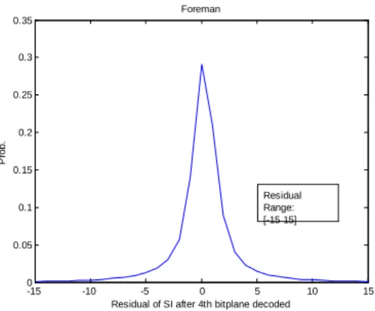
-15 -10 -5 0 5 10 15 0 0.05 0.1 0.15 0.2 0.25 0.3 0.35

Residual of SI after 4th bitplane decoded

P ro b . Foreman Residual Range: [-15 15]

Figure 8.Error distributions when 1st ~ 4th bit-planes are decoded

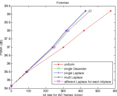
We can see how the error distribution changes as more bit-planes are decoded in Figure 8. When more bit-planes are decoded, errors are more concentrated and their means are more closed to 0. Now we try to use different Laplace models for each bit-plane. The R-D curve is shown in Figure 9. We can see that the performance is worse than using one distribution parameter value for all bit-plane. It is even worse than using a single Gaussian model for all bit-planes when bitrate exceeds 350 kbps. It may be because that when using different Laplace models for each bit-plane, the Laplace model for less significant bit-plane will be more concentrated because the error distribution of SI when decoding less significant bit-plane is more concentrated. However, actually when decoding less significant bit-plane, the probability of bit error is larger. So, the error model does not fit the actual error distribution, and it decreases the performance.

Figure 9.R-D curve of ‘Foreman’ when different Laplace models are used for each bit-plane

3.2 LDPCA Decoding

3.2.1 LLR (Log Likely-hood Ratio) Values

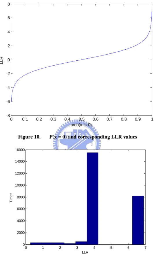
The LDPC decoding of each bit x in a bitplane of the W-Z frame is based on the LLR (log likely-hood ratio). The relationship of P(x=0) and the corresponding LLR values are shown in Figure 10. When the channel error is small, P(x=0) will not be closed to 0.5, and absolute value of LLR will be far from 0. In this situation, fewer W-Z bits will be necessary to correct the errors in side information. So, in this section, we investigate the LLR values of every pixel in the Foreman sequence to estimate the number of W-Z bits required for error correction.

0 0.1 0.2 0.3 0.4 0.5 0.6 0.7 0.8 0.9 1 -8 -6 -4 -2 0 2 4 6 8 prob(x is 0) L L R

Figure 10. P(x = 0) and corresponding LLR values

0 1 2 3 4 5 6 7 0 2000 4000 6000 8000 10000 12000 14000 16000 LLR T im e s

Figure 11. Absolute values of LLR when decoding 1st bit-plane of ‘Foreman’

2nd frame

We plot the histogram of absolute values of LLR when decoding 1st bit-plane of the 2nd frame of the ‘Foreman’ sequence in Figure 11. Most of the values are around

3.89 and 6.91. We want to see the amount of pixels with small absolute values of LLR, because when the absolute values of LLR are small, it means these pixels are considered noisy. We discover that these pixels are all with side information pixel values near 127 (from 124 to 133). 127 is the threshold between 0 and 1 in the 1st bit-plane. We show the scatter plot of side information value and absolute value of LLR when decoding 1st bit-plane of ‘Foreman’ 2nd frame in Figure 12. The scatter plots for 2nd and 3rd bit-planes are in Figure 13 and Figure 14. We can see that pixels with small LLR values are all with side information values near the threshold of particular bit is ‘0’ and ‘1’. We call this threshold ‘crossing threshold.’

Figure 12. Absolute value of LLR and pixel value of side information when

Figure 13. Absolute value of LLR and pixel value of side information when decoding 2nd bit-plane of ‘Foreman’ 2nd frame

Figure 14. Absolute value of LLR and pixel value of side information when

decoding 2nd bit-plane of ‘Foreman’ 2nd frame

Larger absolute values of LLR means less correction bits are needed, but actually it is not certain that their errors are small. Bitrate may be wasted for these pixels.

Those pixels with large absolute LLR but large errors are called under-corrected pixels, and pixels with small absolute LLR but small errors are called over-corrected pixels.

For 2nd frame of foreman sequence, we set the threshold of side information error at 5 and 25. So when side information is large than 25, we call it “Large error”, while side information is smaller than 5, we call it “Small error.” We also set the threshold of |LLR| at 3.89. These thresholds are decided based on the distribution of side informaion and LLR values of this particular frame. After the thresholds are decided, we can calculate the percentage of over-corrected pixels and under-corrected pixels and the result is in Table 2. When more bitplanes are decoded, the percentage of over-corrected pixels is also increased. Although there is only 10% of pixels are over-corrected, we want to see how these pixels affect the performance.

Table 2. Percentage of over-corrected pixels and under-corrected pixels of foreman 2nd frame Over-corrected Under-corrected 1st bitplane 5.56% 0.6% 2nd bitplane 6.03% 0.68% 3rd bitplane 10.3% 2.13%

3.2.2 Over-Corrected Pixels

An experiment is conducted to see how these over-corrected pixels affect bitrate. To achieve this, we peek at pixel values of the original WZ frames. For pixels whose side information is near ‘crossing threshold’ and error smaller than 5, we assign side information pixel values to the original frame pixels and do LDPCA encoding and

decoding. Here we change LLR of these pixels to 3.89 or -3.89. In this experiment, the key frames are encoded using H.264 intra encoder with QP 25. The two R-D curves are shown in Figure 15. One of them is the original R-D curve. Another one is the R-D curve when we ignore pixels with side information near crossing threshold and small residuals. It represents the ideal situation where for all pixels with small residual, the side information values are not near crossing threshold. From the experimental results, we can see that the value of side information is impartment and affects bitrate much although there is only about 10% of pixels are modified. As bitrate increases, the R-D performance difference increases.

But this experiment could not happen in real world because the encoder cannot detect which pixels need to be modified. A practical solution is for the decoder to ignore pixels near ‘crossing threshold’ when it performs LDPCA decoding. So the encoder does not have to detect and modify these pixels and re-encode them. In this experiment, the decoder set LLR values of these pixels to 3.89 or -3.89. These pixels are not modified after each bit-plane is decoded, and when the LDPCA decoder tests convergence or checks syndromes, these pixels are ignored. Here we use ‘Carphone’ sequence to test, and the R-D curve is in Figure 16.

Figure 15. R-D performance when ignoring pixels with side information near ‘crossing threshold’ and small residual

Figure 16. R-D performance when decoder ignore pixels with side

information values near ‘crossing threshold’

We can see that the performance is worse when decoder ignore pixels with side information values near ‘crossing threshold.’ This is because there are too many syndromes not checked because they contain information of ignored pixels. So, when

LDPCA iterative termination condition is reached, it finishes decoding with errors, and more syndrome bits are requested.

3.2.3 Prioritized Decoding of Side Information Pixels

Based on the previous experiments, we propose a way to perform prioritized correction of side information. We can divide pixels into two groups, and the two groups are in different LDPCA coding blocks so we can deal with them separately. In order to implement this approach, there are some key issues which need to be resolved. First, how can the DVC codec classify the side information into pixels into two groups? Secondly, how to encode syndrome bits of different groups of pixels separately at the encoder?

The decoder can see the side information; it can partition pixels into two groups and send the group information back to the encoder. If the group information is at pixel level, then the amount of bits used to describe group information would be too high. Therefore, we compute the group information at macroblock level. For each macroblock in a frame, it will be classified into one of two groups.

When the encoder receives group information, it will rearrange macroblocks in a frame. The macroblocks belong to the same group will be channel-coded together, so they will be LDPCA encoded within a block. This way, the LDPCA syndrome bits can be spent on the area where the residual values are large, and errors are corrected more efficiently. In chapter 4 we will describe the proposed method of classifying and re-ordering macroblocks in detail. The experimental results will be given in chapter 5.

Chapter 4: System Architecture

In this chapter, the proposed DVC codec will be described in details. Our DVC codec is implemented in C. Macroblocks in a frame will be classified into different groups according to their side information quality. Each group of macroblocks will be LDPCA-coded in the same coding block. So we can encode and decode each group of macroblocks according to their significance (priority) in R-D improvement. The prioritized channel decoding will enhance the performance because WZ bits are requested more efficiently.

We have implemented both pixel domain and frequency domain DVC systems. In the following sections, we will use frequency domain DVC codec to explain the proposed scheme, and then the difference between pixel and frequency domain approach will be described.

4.1 System Block Diagram

The system block diagram of the proposed frequency domain DVC codec is shown in Figure 17. First, a sequence will be divided into key frames and WZ frames. Odd frames are key frames and even frames are WZ frames. Key frames are encoded and decoded using H.264 main profile intra coder. The version of H.264 codec we use is JM 9.0. The QP values are determined based on quantization matrices used for WZ frames.

The decoder uses key frames it has received to generate side information of WZ frame. Then it will classify macroblocks into two groups, SA and SB, based on side

information quality. SA contains 25% macroblocks with worse side information

quality and SB contains 75% macroblocks with less side information error. The

on some cues available. The classifying result will be sent to the encoder. And then the encoder will group macroblocks in WZ frame while the decoder will group macroblocks in side information according to the classifying result. Macroblocks in same group will be gathered together.

Macroblocks in WZ frame and side information are then transformed and quantized by encoder and decoder. The encoder will calculate quantization interval for each band and send the values to the decoder. So the encoder and decoder use the same quantization interval to quantize coefficients.

The quantized coefficients of WZ frame and side information are then split into bit-planes. Each bit-plane of a WZ frame will be LDPCA encoded by the encoder. The WZ bits are stored in a buffer and they will be requested by the decoder.

Figure 17. System flow of our transform domain DVC codec

The decoder will request for WZ bits in the buffer and perform LDPCA decoding, and the detail will be described later. Only macroblocks in SA are decoded.

After every bitplanes of every coefficient bands are decoded, these decoded coefficients will be inverse transformed and macroblocks will be rearranged to original order. The following sections will describe the details in each step of the

proposed algorithm.

4.2 Side Information Generation

As we describe above, key frames are coded by H.264 intra coder and sent to the decoder. The decoder uses neighboring key frames to interpolate side information of center WZ frame.

Steps of side information generation are described in this section.

Figure 18. Motion estimation for neighboring key frames

Figure 19. Bi-directional motion adjustment

In step one, motion estimation is performed for two neighboring key frames, as shown in Figure 18. Size of macroblock is 16 by 16, search range is ±32, and motion vector accuracy is at is full pixel precision. The search range is larger than traditional video codec because the time distance between key frames is 2. In this step, we only use forward motion estimation to guess the motion field of WZ frame. There are many works we can do in order to make the motion field more closed to true motion.

In step two, refer to DISCOVER’s DVC codec[18], a bi-directional motion adjustment is performed, and the search range is ±10 with half pixel precision. The half pixel values are calculated using H.264 six-tap filter. The search range is smaller so the adjusted motion vector will not be very far away from original motion vector.

As in Figure 19, if the motion vector obtained in step one motion estimation is (X1, Y1)

and the center of macroblock in WZ frame is (Px, Py), then when performing

bi-directional motion adjustment, the center is fixed and motion vectors (X1+dx,

Y1+dy) with dx and dy within range ±10 are searched. The new motion vector (X’, Y’)

will make SAD (sum of absolute difference) value of macroblock pair in neighboring key frames smallest. Every motion vectors obtained in step one will be modified in this step.

In step three, median filter is applied in order to smooth the estimated motion field. This step is also suggested by the DISCOVER DVC codec [16]. After motion estimation for neighboring key frames and bi-directional motion adjustment, for each macroblock, its motion vector and the motion vectors of eight-connected macroblock neighbors are listed. Then a median motion vector is obtained among these motion vectors. When deciding which one of them is the median, a weight for each motion vector is used.

There are eight neighbors with motion vectors m1 to m8, and motion vector of the

center macroblock is m0. For the center macroblock, the motion vector m0 will point

to two macroblocks in neighboring key frames, and SAD of these two macroblocks is s0. When m0 is replaced by m1 to m8, the SAD of neighboring two macroblocks will

be s1 to s8. The weight value wi of the neighbor motion vector mi is defined as s0/si. So,

if mi makes neighboring macroblocks similar, then its weight is larger. After median

motion vector is obtained, the motion vector will be replaced with this median motion vector. Now the motion field of WZ frame is obtained and side information will be interpolated based on this motion field.

Average of macroblocks in neighboring frames is interpolated to generate side information. The SAD values of macroblock in neighboring key frames are recorded for macroblock classification later. Now, there are some pixels which have more than

one projections from neighboring key frames. For such pixels, the average of interpolated values of all projections is used as the side information. Some pixels do not have projections at all, and these pixels remain unfilled as holes in the side information..

Two hole-filling procedures are applied to complete the side information. For the first procedure, if the Manhattan distance between the hole and nearest filled pixel is within 25 pixels, then the motion vector of this filled pixel is used by the hole for motion compensation from neighboring key frames. Otherwise, another hole-filling procedure is applied. Distance upper bound is chosen as 25 pixels because we do not want to use motion vectors of pixels too far away.

The remaining holes will be filled by the second hole-filling procedure. Now for each macroblock in side information, calculate the percentage of holes. If the percentage of holes is less than 40 percent, then motion estimation for this macroblock and previous key frame in display order will be performed. Only filled pixels are used to calculate SAD, and we achieve this by using a mask to ignore difference values at holes when calculating SAD. The macroblock size is 16 by 16 and the search range is ±32. The macroblock with smallest SAD in previous key frame is located and the corresponding pixels in this macroblock will be used to fill the holes in side information.

If the percentage of hole is larger than 40 percent, then the size of macroblock will be enlarged by 2 each time until it reaches 32 by 32. The percentage of holes is 40 percent at most because when there are too many holes in one macroblock, then the valid pixels used to find motion will be minority. Thus an incorrect motion vector will be obtained. The size of macroblock used to find motion vector for holes can not be too large, too. When the macroblock size is too large, the results of motion estimation will be bad because pixels within one macroblock in practice have

different motions.

4.3 Macroblock Classification and Grouping

Given the generated side information, the decoder will classify macroblocks into groups SA and SB. SA contains 25% macroblocks with worse side information quality

and SB contains 75% macroblocks with less side information error. For QCIF

resolution sequences, there are 24 macroblocks in group SA and there are total 99

macroblocks. And this makes each bit-plane of each coefficient band of group SA

contains 384 bits (24 macroblocks are equal to 384 4 by 4 blocks,) and the LDPCA block size we use when only group SA is decoded is 396. If we pick up 25

macroblocks for group SA, then each bit-plane of each coefficient band of group SA

will contain 400 bits and this is larger than 396.

Because the decoder does not have the original WZ frames, therefore it must estimate the quality of side information in order to classify macroblocks. Many features of the side information image, such as the motion field variance, the number of edges or corner points, and the SAD values of macroblocks in neighboring key frames, can be used as estimates for classification.

To obtain motion field variance, we need dense motion field. When generating side information, motion vectors of macroblock size 16 by 16 is generated. And then a 16 by 16 macroblocks is divided to four 8 by 8 blocks. Start from motion field already obtained, motion estimation similar to bi-direction adjustment above is performed and the search range is ±10. So, for each macroblock, there will be four motion vectors, and we get a dense motion field. We can further divide each 8 by 8 macroblock to four 4 by 4 macroblocks and get a more dense motion field. After dense motion field is obtained, motion vector length variance of every macroblock is calculated and this variance is used to classify macroblocks. When the variance is larger, we think the

side information quality of this macroblock is worse.

To obtain number of edges and corner points, we use Sobel filter to get edges and use Harris corner detector to get corner points. The Sobel filter size is 3 by 3, and the setting of Harris corner detector is radius 3, sigma 1, and threshold 10 for all test sequences. The values of radius and sigma are recommended by the author of Harris corner detector and the threshold is set as 10 so there will not be too many annoying corner points. When there are more corner points or edges in a macroblock, we think the side information quality is worse. We use these features as cues because we have observed that for Foreman sequence, macroblocks containing these features have worse side information quality.

To obtain SAD of macroblocks in neighboring key frames, we do not do additional works because we obtain these values when generating side information. When SAD of macroblocks in neighboring key is larger, we think the quality of side information is worse. And this is because side information quality is proportioned to SAD of macroblocks for many pixels statistically, especially when motion is well guessed.

After trying these cues, we have discovered empirically that SAD of macroblocks in neighboring key frames is a good cue for the decoder to pick up worse macroblocks, as shown in Figure 21. Several sequences are tested in pixel domain with lossless key frames, and the optimal R-D curve is the case where we take a peek at the original WZ frame and choose macroblocks that have the worst side information.

The decoder will use 99 bits to descript classifying result and the result will be sent to the encoder. Bit ‘0’ represents group SA and bit ‘1’ represents group SB. The

decoder will rearrange macroblocks in the side information and macroblocks of same group will be gathered together. The encoder will also rearrange macroblocks in WZ

frame in the same way.

Figure 20. Macroblock rearrange

The macroblocks of group SA are placed at top of the frame, and macroblocks of

group SB are placed at bottom of the frame, as shown in Figure 20. The order of

macroblocks of same group is maintained in scan-line order. So if there are 2 macroblocks of group SA, m1 and m2, and m1 precedes m2 before the rearrangement.

Then m1 will precede m2 after the rearrangement. After macroblock reordering and

grouping, macroblocks of the same group will be packed in the same LDPCA block for W-Z frame coding.

0 50 100 150 200 250 37 38 39 40 41 42 43 bit rate (kbps) P S N R ( d B ) Hall Original By SAD

By motion field length variance (8x8) By motion field length variance (4x4) By number of corner points Optimal 0 100 200 300 400 500 600 26 28 30 32 34 36 38 40 bit rate (kbps) P S N R ( d B ) Ice Original By SAD

By motion field length variance (8x8) By motion field length variance (4x4) By number of corner points Optimal 0 20 40 60 80 100 120 140 160 180 200 40.5 41 41.5 42 42.5 43 43.5 44 44.5 bit rate (kbps) P S N R ( d B )

Mother and Daughter

Original By SAD

By motion field length variance (8x8) By motion field length variance (4x4) By number of corner points Optimal 0 50 100 150 200 250 300 350 400 450 42.5 43 43.5 44 44.5 45 45.5 46 bit rate (kbps) P S N R ( d B ) Salesman Original By SAD

By motion field length variance (8x8) By motion field length variance (4x4) By number of corner points Optimal 0 20 40 60 80 100 120 140 160 47.2 47.3 47.4 47.5 47.6 47.7 47.8 47.9 48 48.1 48.2 bit rate (kbps) P S N R ( d B ) Grandmother Original By SAD

By motion field length variance (8x8) By motion field length variance (4x4) By number of corner points Optimal 0 50 100 150 200 250 300 33 34 35 36 37 38 39 40 41 bit rate (kbps) P S N R ( d B ) Highway Original By SAD

By motion field length variance (8x8) By motion field length variance (4x4) By number of corner points Optimal 0 50 100 150 200 250 43.8 44 44.2 44.4 44.6 44.8 45 45.2 45.4 45.6 45.8 bit rate (kbps) P S N R ( d B ) Miss Original By SAD

By motion field length variance (8x8) By motion field length variance (4x4) By number of corner points Optimal 0 20 40 60 80 100 120 140 160 180 200 37 38 39 40 41 42 43 44 45 bit rate (kbps) P S N R ( d B ) News Original By SAD

By motion field length variance (8x8) By motion field length variance (4x4) By number of corner points Optimal