行政院國家科學委員會專題研究計畫 成果報告
具安全通訊與系統防護之無線微型感測網路研發與實作(I)
計畫類別: 整合型計畫 計畫編號: NSC93-2213-E-009-120- 執行期間: 93 年 08 月 01 日至 94 年 07 月 31 日 執行單位: 國立交通大學資訊工程學系(所) 計畫主持人: 謝續平 報告類型: 精簡報告 處理方式: 本計畫可公開查詢中 華 民 國 94 年 10 月 26 日
行政院國家科學委員會專題研究計畫期末報告
具安全通訊與系統防護之無線微型感測網路研發與實作(I)
計畫編號:NSC 93-2213-E-009-120- 執行期間:2004 年 08 月 01 日至 2005 年 07 月 31 日 主持人:謝續平 執行單位:國立交通大學資訊工程學系(所)中文摘要
在本計畫中,我們發現要在無線微型感測網路上加入安全通訊與系統防護機制時,其 能量消耗相當大,因此在電力能源有限無線微型感測網路中,省電機制將會是本計畫很重 要的部份。本計畫為三年計畫,因此,第一年我們設計的重點在於無線微型感測網路的省 電機制。由於無線微型網路硬體的限制,使得傳輸方法的設計成為一種挑戰。在無線微型 網路中,我們希望每一個節點可以儘量延長他們的工作時間,因此,如何設計一個優良的 傳輸方法來延長無線微型網路存活時間成為一個重要的課題。另一方面,我們希望能源消 耗可以平均分配在網路中的各個節點上,讓我們欲監控的環境可以被完整的涵蓋住,並同 時保持網路的最佳連通性。 在本計畫中,我們提出了一個有效率的資料傳輸方法。雖然目前已經有一些傳輸方法 被提出來,但是這些方法都是讓網路節點依據機率來組織網路叢集。這種使用機率決定網 路分佈的方法不能提供一個穩定的叢集散佈,並且能源消耗分散的問題也無法有效的被解 決。本計畫所提出來的方法是使用基地台來組織網路叢集,具有有效利用有限的能源而且 能源消耗可以被平均分散到各個網路節點之特性。模擬的結果顯示,與現有的方法相比較, 本計畫中所提的方法大大地改進能源消耗的議題。Abstract
There are more and more emphases on wireless sensor network in recent years. In wireless sensor network, every sensor node has the capability of sensing, data processing, communication, and operates on its limited irrechargeable battery. In this project, we designed an energy efficient transmission scheme that can distribute the energy consumption evenly on each node to prolong
the lifetime of wireless sensor network. Most of the previous work of this issue use node self-organized with probability to solve the problem, but the probability based approaching cannot provide an evenly distributed energy consumption scheme on each sensor node. In our scheme, we use base station to organize clustering of wireless sensor, and it has the advantages that energy consumption can be distributed evenly. The simulation results showed that our scheme could greatly improve energy consumption than the existing solutions.
1. Introduction
Wireless Sensor Networks (WSN) is a new research on wireless technology. How to route data is an important issue for WSN [26] [27] [28]. Some known researches on routing for Ad-Hoc networks are infeasible for wireless sensor network due to the hardware limitation of the sensor nodes. In this project, we will introduce a new routing scheme for wireless sensor network whose purpose is to reduce energy consumption and distribute the energy cost evenly.
In the following paragraphs, we will introduce the idea of wireless senor network in Section 1.1, and the routing problem in wireless sensor network will be presented in Section 1.2. Furthermore, we will specify our contribution in Section 1.3, and introduce the organization of this report in Section 1.4.
1.1 Wireless sensor networks
With the increasing advances in hardware and wireless network technologies, the small wireless devices will be able to provide access to information anytime and anywhere [6]. The wireless sensor network is a kind of application that is formed with a set of small sensor devices that are deployed in an ad hoc fashion and cooperate on sensing a physical phenomenon. Although the sensor nodes are not reliable, hundreds or thousands of these nodes deployed in the network can provide a high quality and fault tolerant sensing network. It is important in many applications for military or commercial. For example, for a security system, acoustic, seismic, and video sensors can be used to form an ad hoc network to detect intrusions. Sensor nodes can also be used to monitor machines for fault detection and diagnosis.
The differences between wireless sensor network and other wireless networks, such as Mobile Ad-hoc Networks (MANET) are:
The small volume of sensor node causes the critical battery capacity. The energy consumption becomes the most critical issue of the design of sensor node. The energy consumption is often less than 1μW.
(2) Low communication bandwidth:
The bandwidth of wireless sensor network is about 10 – 1000kb/s. It is relative low to the traditional wireless networks.
(3) Limited memory space and computing power:
Due to the small volume and low cost of each sensor node, the memory space and computing power are critically limited. The memory space ranges from several kilo bytes to hundreds kilo bytes. The computing power ranges from 4MHz to 100MHz. (4) The large scale of deployment:
A wireless sensor networks consists of hundreds even thousands of small wireless sensor nodes. Those sensor nodes are deployed in a large wide area for sensing a physical phenomenon.
(5) High node failure rate:
The terrible deployed environment may make sensor nodes easy to be broken, and there may be some obstacles blocked the communication signal and made sensor nodes temporary unavailable.
Wireless sensor networks can contain hundreds or thousands of sensing nodes. It is desirable to make these nodes as cheap and energy-efficient as possible and rely on their large numbers to obtain high quality results. Network protocols must be designed to minimize the energy consumption on sensor nodes. In addition, since the limited wireless channel bandwidth must be shared among all the sensors in the network, routing protocols for these networks should be able to perform local collaboration to reduce bandwidth requirements.
There are lots of applications for wireless sensor networks. In military applications, the wireless sensor network can be used for command, control, and communication. In health applications, they can be deployed on patients to monitor and assist the disabled patients. In commercial applications, they can be used for managing inventory, and product quality monitoring. There are many other applications such as disaster area monitoring, traffic monitoring…etc.
1.2 The transmission in wireless sensor networks
area and the mission is to sense certain data (as shown in figure 1-1). How to send the sensed data back to the base station? We need a good solution that can reduce the energy cost on sensor nodes to keep sensor nodes alive as long as possible.
Figure 1-1: WSN with hop-by-hop routing
For example, one of the methods to route data is that each node which has data to send just forwards the data to its neighboring nodes. It is easy to implement but each node on the data path spends energy on receiving and transferring data. Moreover, every node has to keep awake in order to listen if there is any data forwarded to it. This takes lots of energy and makes the nodes die quickly. Actually, not all nodes need to keep awake to maintain the network connectivity, we can organize a set of nodes and each of the nodes is responsible to a region and those regions cover all the nodes in the deployed area to collect all the data sensed by sensor nodes. This is what we called “clustering”.
Generally speaking, cluster-based routing protocol has following advantages: (1) Energy saving for cluster member
Each cluster has a cluster head which will keep awake to collect data from the other nodes in this cluster. Cluster member (nodes except cluster head) can turn off the radio module until it senses any data. Therefore, if there is nothing sensed, the cluster members spend extremely low energy during the round.
(2) Easy to maintain routing table
For cluster members, each of them only need to remember which node is the cluster head. This takes less memory space then other routing approach, e.g. DSR, AODV. This is critical for sensor nodes due to its small RAM size.
(3) Data aggregation at cluster head
Sensor nodes may sense much redundant data in the same region. Cluster head can perform data aggregation function to reduce the data. Cluster head can spend less energy since the data has been reduced.
Wireless sensor nodes are expected to work as long as possible so how to prolong the network lifetime is a very important issue in wireless sensor network. Cluster-based routing protocol is a good method which can save energy easily because of the features mentioned above. There are some cluster based solutions [1] [2] [3] and we will introduce them in section 2.
1.3 Contributions
We presented a new energy efficient routing scheme for wireless sensor network. Unlike the traditional cluster based routing schemes, we use the base station to organize the cluster distribution instead of node self election. By our scheme, sensor nodes can save more energy than some other solutions so that the network lifetime can be increased. Moreover, the energy cost is distributed evenly to each node. This makes nodes can live longer to keep the deployed area being covered.
We did some simulations for our scheme and the results showed that the properties we claimed are true. In terms of network lifetime, our scheme has 60%-90% improvement compare to LEACH and HEED. By our scheme, the lifetime of wireless sensor network can be maximized. Power saving is an important issue in wireless sensor network and we did a well improvement in this field.
2. Related work
In this section, we will introduce some known clustering schemes first and then take a look at some other techniques used in our scheme.
2.1 Clustering algorithms
Several clustering schemes for Ad-hoc network have been proposed in recent years [7] – [15]. They are not really suitable for wireless sensor network because of sensor node is a low cost device with poor resource, e.g. slow CPU, less RAM and low-capacity battery. For wireless sensor networks with a large number of energy-constrained sensors, it is very important to design a fast algorithm to organize sensors in clusters to minimize the energy used to communicate information from all nodes to the base station. The benefits of dividing nodes in clusters are:
nothing to send in order to save energy. A node in sleeping mode consumes energy far less then in transmitting or receiving mode [6].
(2) Easy to maintain routing table: cluster members only need to remember which node to relay the sensed data. There is no enough memory space for nodes to store a huge routing table.
(3) Data aggregation can be performed at cluster head: In some environments or applications, there is lots of redundant data may be produced. Perform data aggregation can reduce the data to save energy or network bandwidth.
There are some known clustering schemes for wireless sensor networks such as LEACH [1], HEED [2], and Seema et al proposed [4]. LEACH is proposed firstly and formed an example for solving clustering problem in sensor networks.
In LEACH, sensors elect themselves as cluster heads with some probability and broadcast their decisions. The remaining sensors join the cluster of the cluster head that requires minimum communication energy. This algorithm allows only 1-hop clusters to be formed.
They have provided simulation results showing how the energy spent in the system changes with the number of clusters formed and have observed that, for a given density of nodes, there are a number of clusters that minimizes the energy spent. But they have not discussed how to compute this optimal number of cluster heads and the proposed algorithm can not guarantee that the formed cluster in each round is optimal. The algorithm is run periodically, and the probability of becoming a cluster head for each period is chosen to ensure that every node becomes a cluster head at least once within 1/P rounds, where P is the desired percentage of cluster heads. This ensures that none of the sensors are overloaded because of the added responsibility of being a cluster head.
HEED (Hybrid, Energy-Efficient, Distributed), like LEACH, nodes use a probability to elect itself to become a cluster head and then broadcast the head announcement to its neighboring nodes. After nodes received the announcement, they can select one of the heads to join in and start to transmit data to the cluster head. HEED also has to rotate the cluster distribution every TCP+TNO seconds. The difference between LEACH and HEED is that HEED considered the residual energy when selecting the cluster head. They made several experiments in the evaluation section and the result showed that their scheme can perform better than LEACH.
In [4], each sensor in the network becomes a cluster head (CH) with probability p and advertises itself as a cluster head to the sensors within its radio range. They call these cluster heads the volunteer cluster heads. This advertisement is forwarded to all the sensors that are no more than k hops away from the cluster head. Any sensor that receives such advertisements and is
not itself a cluster head joins the cluster of the closest cluster head. Any sensor that is neither a cluster head nor has joined any cluster itself becomes a cluster head called forced cluster head.
Because the advertisement have limited forwarding to k hops, if a sensor does not receive a CH advertisement within time duration t (where t units is the time required for data to reach the cluster head from any sensor k hops away) it can infer that it is not within k hops of any volunteer cluster head and hence become a forced cluster head. Moreover, since all the sensors within a cluster are at most k hops away from the cluster-head, the cluster head can transmit the aggregated information to the processing center after every t units of time. This limit on the number of hops thus allows the cluster-heads to schedule their transmissions. In this scheme, node does not demand clock synchronization. The energy used in the network for the information gathered by the sensors to reach the processing center will depend on the parameters p and k of the algorithm where p is the probability for a node to become a cluster head and k is mentioned above means “k” hops to forward the advertisement.
As we can see, the common point of these known schemes is that they are node self-organized based on certain probability. But the fatal flaw is that nodes self-organized based on probability scheme can’t provide optimal clusters and the inter-cluster communication overhead actually wasted lots of energy.
2.2 Positioning algorithms
Position information is very useful in wireless sensor network. Usually the sensors are deployed arbitrarily so we have no idea about the position of the nodes. If we can know the position of the nodes in some applications, it is useful and can help us to do something. Many algorithms were developed in recent years [20] [21] [22] [23] [24] [25]. These researches showed that positioning in wireless sensor network is possible and can be implemented in practice. In our environment assumptions (section 3.1), we made such assumption: All nodes are stationary and
have the ability to calibrate distance with each other. In order to show the assumption is feasible,
we briefly introduce the challenge of positioning problem and some approaches in this section. Localization approaches typically rely on some form of communication between reference points with known positions and the receiver node that needs to be localized. We classify the various localization approaches into two broad categories based on the granularity of information inferred during this communication. Approaches that infer fine grained information such as the distance to a reference point based on signal strength or timing measurements fall into the category of fine grained localization methods and those that infer coarse grained information such as proximity to a given reference point are categorized as coarse grained localization methods.
Koen Langendoen and Niels Reijers made comparison for some positioning algorithm designed for wireless sensor network. They focused on the non-infrastructure based algorithm. Through their observation, all positioning algorithms can be organized in a common, three phase structure: (1) determine node to anchor distances, (2) compute node positions and (3) optionally refine the positions through an iterative procedure. They presented a detailed analysis comparing the various alternatives for each phase, as well as a head-to-head comparison of the complete algorithms. The main conclusion is that no single algorithm performs best; which algorithm is to be preferred depends on the conditions (range errors, connectivity, anchor fraction, etc.). According to their experiment result, they showed that in some combinations the position determination can be done within an acceptable error range.
3. Proposed scheme
We proposed Cluster-Based Energy-Efficient Transmission scheme for wireless sensor network (C-BEET). In sensor networks, nodes are usually equipped with slower CPU, small memory and low-capacity battery. Due to the resource constraint, we need to design a routing scheme for sensor nodes to send back their sensed data. The aim of the proposed scheme is to reduce total power consumption of the network and prolong the network lifetime. In this section, we will describe how to divide nodes into clusters and how to assign nodes to join certain cluster in detail.
3.1 Environment description
In most of the sensor network applications, sensor nodes are deployed in the field in order to sense data. All the sensed data are sent back to the base station where is far away from the field. We firstly describe a typical sensor network and make some assumptions about the sensor network.
We assume the following properties about the sensor network: (1) Base station can reach all nodes in the sensor field via hopping.
(2) All nodes are stationary and have the ability to calibrate distance between each other. (3) Localization algorithm is performed and all nodes report their locations to BS via
flooding.
(4) Links are symmetric, i.e., two nodes u and v can communicate using the same transmission power from u to v or from v to u.
(5) The RF model used in this thesis is the same as LEACH [1] described as below: k E k E d k k E d k E elec Rx amp elec Tx * ) ( * * * ) , ( 2 = + = ε
Operation Energy Dissipated
Transmitter
Electronics(ETX-elec) Receiver
Electronics(ERX-elec) ETX-elec = ERX-ele = Eelec
50 nJ/bit1
Transmit Amplifier 100 pJ/bit/m22 Table 3-1. The parameters of the RF model
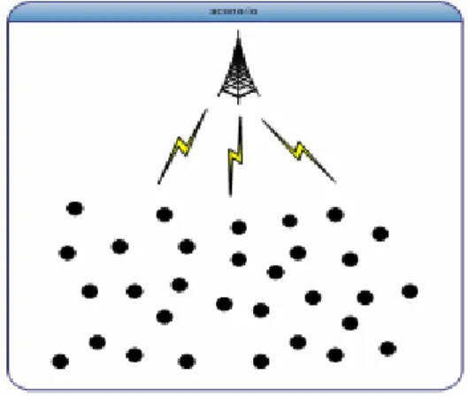
Figure 3-1: The WSN environment
Figure 3-1 showed the sensor network environment briefly. The black points are sensor nodes and the “tower” represents the Base Station. All deployed nodes are responsible for sensing data. After the nodes sensed any data, they need to send back to BS. Of course the nodes can send it back hop by hop individually but due to the large power consumption of RF transmission [6], hop by hop transmission takes lots of energy at each hop on the path. In order to prolong the network lifetime, to design an efficient routing scheme for wireless sensor network is necessary.
3.2 The cluster-based energy efficient transmission scheme (C-BEET)
1 1 nJ = 10-9 J 2 1 pJ = 10-12 J
In this section, we will describe the C-BEET scheme. Unlike the known cluster-based scheme mentioned in the related work section, C-BEET is controlled by base station. In LEACH [1] and HEED [2], nodes elect itself to be a cluster head with certain probability. After that, the head node needs to broadcast the head advertisement to their neighboring nodes and the neighboring nodes also need to listen if there is any head advertisement in the air. Moreover, members need to send a “join confirmation message” to the cluster head which they want to join in. We called it as “inter-cluster communication” and this incurred lots of energy lost. Besides that, cluster members (all nodes except the cluster head) did not know the distance between cluster head and themselves so the cluster members need to emit signal at certain power level to make sure cluster head can receive the data. But the signal strength may exceed the actual distance they need. According to the radio model, energy consumption is proportion to distance square, so if the cluster members know the distance to the head precisely, there is more energy to save.
According to those drawbacks mentioned above, C-BEET, a cluster-based energy-efficient transmission scheme, improved those issues based on the following properties:
(1) Sensor nodes don’t need to elect themselves to be the cluster head instead of receiving the “Head Locations (HLs)” from the base station
(2) Non-head nodes can compute the distance between the head and themselves according to the head coordinate listed in the HLs.
The first property eliminated the inter-cluster communication because the cluster heads are assigned by the base station so the nodes need not to compute if it should be the cluster head. The assigned cluster head also needs not to broadcast the head advertisement because after the other nodes received the HI, they just compute the distance to those heads and chooses the shortest distance to join the cluster head. So there is no head advertisement and join cluster confirmation message in the network. This eliminated the inter-cluster communication indeed.
Since the cluster member can get the head coordinate from the HI and count the distance to the head, nodes can adjust their emit power just fit the distance to the head so that can use the minimum power to reach the cluster head. This implied whole network run under the minimum power consumption condition.
The basis concept of C-BEET is described here and we will detail the C-BEET in 3.3.
3.3 Insight into the C-BEET
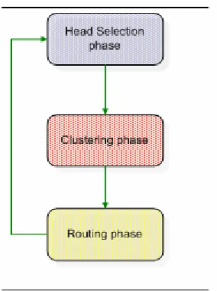
Let’s look inside how C-BEET works. We divide C-BEET into three phases, they are: head selection phase, clustering phase and routing phase. Figure 3-2 showed the relationship of the two
phases. In head selection phase, all nodes stay in receiving mode to receive the “Head Locations” broadcasted from the base station. After receiving the head information, nodes jump to clustering phase.
In clustering phase, nodes are divided into clusters according to the head information received in the head selection phase and data can be delivered to the cluster head. While time Ti
has passed since clustering phase, nodes jump back to head selection phase in order to change the cluster head and prevent the head nodes from exhausting their energy. After that, nodes go to clustering phase again and the network iterates in clustering phase and head selection phase until the network ends.
Figure 3-2: Relationship of the three phases
3.3.1 Head selection phase
Nodes in this phase are waiting for the “Head Locations” sent by the base station. After BS acquired the position of the nodes, it starts computing the best cluster for the nodes disseminated in the field. According to the RF model, energy consumption is proportion to distance square (E α D2) so the problem of clustering can be reduced into the “K-median problem” which is to minimize
∑ ∑
= ∈ k i u Ci i h u d 1 ) ,( , in other words, the goal is to minimize the total distance which
nodes need to send. The detail of the clustering algorithm will be described in section 3.4 and now we keep on explaining to the head selection phase.
When the base station computed the best clustering result, it has to send the information to the nodes. Instead of sending each node which clusters it belongs, base station sends “Head Location” contained the data of each cluster head. The reason why we use a single “Head
Locations” is that if the base station sends to each node which cluster to join individually, it wastes a lot of energy for all the nodes because each node must listen to the base station and distinguish if the message is for it. So we use head locations instead of sending to each node individually. Although nodes would sacrifice slight computation for determining which node is the cluster head, it is worth for saving the energy of entire network.
3.3.2 Clustering phase
The mission of clustering phase is to form the clusters and each node has to find out its cluster head. Firstly, let’s see what is included in the “Head Locations”. Head locations must list all the cluster head data such as node ID, position. The format of the message is:
(IDBS, PBS) || (ID1, P1) || (ID2, P2) || … || (IDk, Pk)
(IDBS, PBS) means base station identification which can help node to know the source of this head location. The pair (IDn, Pn) means cluster head n and its position. If the network is divided into k clusters, there should be k pairs in the head information. The position can be represented as relative coordinate or longitude and latitude. We suggest using relative coordinate that is more convenient to compute the distance with each other.
After receiving the head locations, nodes are classified to cluster heads and members. Nodes whose ID are listed in the head locations become cluster heads and others become cluster member. As long as a node becomes a cluster head, it has to stay in listening mode to listen if there is any data from cluster members. Cluster members decide their cluster head by computing the distances to the heads listed in the head information. Of course they select the nearest cluster head to be their cluster head.
To compute the distance between nodes, just use the distance formula in two dimension
space: 2 1 2 2 1 2 ) ( )
(x −x + y −y , where (x1, y1), (x2, y2) are nodes in a plane. Since nodes know their own position and the head positions are listed in the head information, they can compute
2 2 ,Y HLs ( h) ( h) XhMinh X X Y Y − + − ∈
, where HLs means Head Information, (Xh, Yh) is the coordinate of nodes listed in HLs and (X, Y)∈CM(Cluster Members).
parent. Note that there is no any communication between members and cluster head except the data during the clustering phase. Unlike some known schemes [1] [2], to join in a cluster doesn’t need sending any message to cluster head in our scheme. Because the cluster head will keep listening during the clustering phase, so the cluster member just need to remember which node is its cluster head and send data to the cluster head whenever they want to send data. Therefore, the inter-cluster communication mentioned in section 3.2 can be eliminated.
Since every node can compute the distance to the cluster head, they can adjust their radio transmission power to cover the range from themselves to the cluster head. As we have mentioned before, the distance is one of the factor that can influence the energy usage. So minimizing the transmitting distance implies that the transmitting power of each node can be minimized. This is one of the reasons why our scheme can save energy indeed.
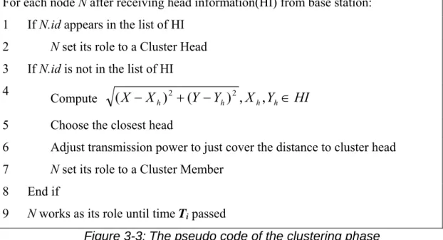
In this section, we have described how clustering phase works in detail. At last, we compose the procedure of clustering phase into the following pseudo code:
For each node N after receiving head information(HI) from base station: 1 If N.id appears in the list of HI
2 N set its role to a Cluster Head
3 If N.id is not in the list of HI
4
Compute (X −Xh)2 +(Y −Yh)2,Xh,Yh∈HI 5 Choose the closest head
6 Adjust transmission power to just cover the distance to cluster head
7 N set its role to a Cluster Member
8 End if
9 N works as its role until time Ti passed
Figure 3-3: The pseudo code of the clustering phase
3.3.3 Routing phase
In this phase, we describe how cluster heads send back the data to base station. After clustering phase, the nodes are formed into clusters. Cluster heads are responsible for receiving data from cluster members. There are two situations that how cluster heads send the data to base station: cluster heads can reach base station or not.
If the base station is in the transmission range of the cluster head, the cluster head can send the data to base station directly. In the other case, cluster head can not transmit data to BS directly
so we designed an approach to solve this situation.
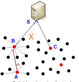
Figure 3-4: Hopping via cluster heads
As shown in figure 3-4, assume that cluster head A cannot reach base station directly; we have to find out a path for the head to transmit the data. The position of the cluster heads and base station are known by HLs, so the node A can find out another that in close to base station. If there is another cluster head B, A can compute the angle between B, A and base station S which is ∠ BAS by the inner production formulation:
The smaller angle θ means that the cluster head B is close to the lineAS. We want to find another head which is near the line AS and is closest to BS. So that, A can compute the angle in the HLs and find out which cluster head can fit the condition.
3.4 Clustering algorithm
Firstly, let’s review the power consumption model in section 3.1:
2 * * * ) , (k d E k k d ETx = elec +εamp
Eelec and εamp are fixed values so the power consumption of sending k bits data is proportion to the d2. Therefore, nodes have to use more energy if they want to send data to a longer distance. With this inference, to shorten the transmitting distance can save energy for entire network. AS AB AS AB⋅ = θ cos
In our environment, sensor nodes are spread in the field and we want to divide them into several clusters. In order to shorten the total distance from cluster members to head, we can reduce the problem to a graph problem. We define a graph:
) , ( EV
G= , where
V = {v | each sensor node in the network},
E = {e | d( u, v), u, v∈V},
d : V × V Æ R
W (u, v) is the weight function of the link between node u and v
And the problem is defined as following:
Pick a set of heads H = {h | h∈V}, |H| = k, to minimize
The object of the problem is to partition N weighted points into k sets such that the sum, over all points n, of the distance from n to the median of set containing n is minimized. This is known to be NP-hard to compute a solution with cost less than a certain constant factor times the optimal cost. There are many researches on this kind of problem [16] [17] [18] [19]. In this thesis, we proposed an algorithm to solving the problem with approximate solutions.
Before we start to introduce the algorithm, let’s see some symbols we defined in this algorithm.
N is the node number of the network
Nu = { e | edges that u can reach}, Nu is the set of neighbors that u can reach. d(u ,v) = the distance between u and v
Edges are directed, asymmetric, euv is the edge from node u to v and euv≠evu W(e) is the weight function of edge e, W(euv) is defined as
) , ( ) 1 ( ) , ( ) ( d v BS E E v u d e W iv rv uv = + − ×
Eiu is the initial energy of node u, Eru is the residual energy of node u
Now, let’s start to introduce our algorithm. The main idea of our algorithm is from the “greedy algorithm.” The sketch of the algorithm is to find out the best neighbors for all nodes at
∑ ∑
= ∈ k i u C i i h u W 1 ) , (beginning by searching the best θ x |V| edges for each node and then check which node is connected by most nodes and then pick it as a head. After that, we eliminate those nodes, the head and those which connect to the head node, from the graph and then repeat to choose the best neighbors until all nodes are eliminated.
First, we transfer the network into a graph G =( EV, ) mentioned above. The first step of the algorithm is to compute the following values:
V
v
N
v,
∈
After computing the neighboring edges for each node, the algorithm then select the best β
x |V| edges for all v in V. According to the weight function W(e), the first βx |V| is the edges
with firstβx |V| small weight. As long as one edge is taken, the algorithm records the source and
the destination of the edge and makes a statistic about the incoming edge for all nodes. Then, pick the node h which is most connected to become a cluster head. Besides that, our algorithm also finds out the set of nodes Nbr which connect to h and eliminate Nbr with h from graph G.
Some nodes may have the same number of edges toward them but we don’t select all of them to become heads. Instead, we defined a function to determine which node is the best to become a head. The function is defined as:
∑
∈ × br N u br ih rh h u d N E E ) , (This function is composed by two parts, one is about energy and the other one is about the distance to head h. First, Erh/Eih considered the residual energy of the node. Nodes with more energy will get more credit from this part. Second part of the function is to compare the average distance from the set Nbr. It is clear that if the edge to h is small, h will get higher score from this equation. The purpose of this function is to select a head with higher residual energy and the shorter distance that cluster members can save their energy.
After the head has been selected, we update the graph G = G – (Nbr ∪ h) and restart the algorithm. The algorithm repeats until G = Φ. All the h in each iteration is the set of heads for the next round.
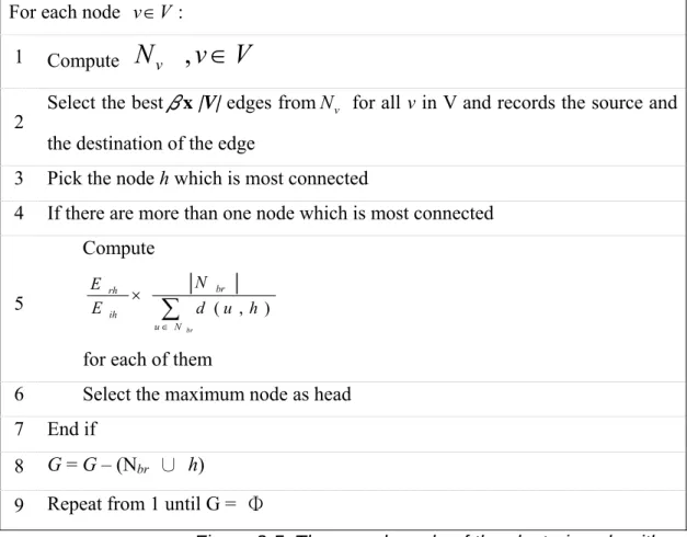
So far, we have introduced the complete cluster algorithm. We arrange the algorithm in pseudo code below:
For each node v∈V :
1 Compute
N
v,
v
∈
V
2 Select the bestβx |V| edges fromN for all v in V and records the source and v the destination of the edge
3 Pick the node h which is most connected
4 If there are more than one node which is most connected
5 Compute
∑
∈ × br N u br ih rh h u d N E E ) , (for each of them
6 Select the maximum node as head 7 End if
8 G = G – (Nbr ∪ h)
9 Repeat from 1 until G = Φ
Figure 3-5: The pseudo code of the clustering algorithm
3.5 Reliability issue
The wireless link between sensor nodes is not as reliable as wired link. The link may fail randomly and it would affect the transmission of the network. We are going to discuss how the link failure affects our scheme.
Let’s review our network architecture first. In our scheme, the sensor nodes are classified as two roles: cluster head and cluster member. The only data flow in our scheme is that cluster member sensed certain data and then sends to cluster head. Under this architecture, we only need to worry about the situation if the link between cluster head and cluster member is still alive. We can classify the link failure into two situations. One is one time failure and the other is permanent failure.
One time failure means the cluster head suffer from some conditions so that the RF system doesn’t work at the time period. Under this situation, the sending node may fail to transmit at the time but it can save the packet into the buffer and wait for the retransmission mechanism. The retransmission mechanism usually implements in the MAC layer so it is out of scope in this thesis.
Permanent failure often happens when the cluster head runs out if its energy. Of course there are many other reasons like nodes broken, damaged, stolen, etc. To deal with these situations, nodes have to notice the condition that if cluster head is no response many times. Most of recent medium access control (MAC) protocols have transmission acknowledgement mechanism. By this mechanism, nodes can know if cluster have received the data. If the MAC doesn’t get the acknowledgement many times, it shows the cluster head have been dead. In such case, cluster member just give up current round and wait for next round comes. It will increase the overhead of the cluster members slightly. Therefore, the reliability issue can be solved easily.
3.6 Summary
In this section, we started with introducing the environment first and then described the difference between traditional routing schemes with our scheme, centralized energy efficient routing scheme (C-BEET). By the properties of C-BEET, the advantage we stated is obvious and reasonable.
Afterward, we introduced the C-BEET in detail. The C-BEET contains three phases: initialization phase, head selection phase and clustering phase. These three phases form C-BEET and is essential for achieving the characteristics in our goal. Moreover, we designed a greedy algorithm in the head selection phase to select which are the best nodes to become cluster heads and then divide other nodes into clusters. We will perform some experiments in the following section to evaluate the efficiency of the algorithm in terms of network lifetime, transmission distance and energy dispersion.
4. Evaluation
In this section, we will evaluate the performance by simulation. Also, we will compare C-BEET with other related schemes. We implemented LEACH, HEED and C-BEET in this project and did variety of experiments to show the merits of C-BEET.
The following paragraphs are organized as: section 4.1 describes the parameters of the simulator, 4.2 shows the difference between C-BEET and other schemes, 4.3 we discuss some important issues in wireless sensor network and explain how C-BEET achieve those properties that we have mentioned earlier.
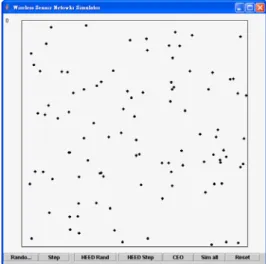
We implemented LEACH, HEED and C-BEET in JAVA. Initially, we put 100 sensor nodes with 0.5 Joule energy in a 50m x 50m field. The distribution of the sensor nodes are randomly calculated by the JAVA library, Math.random(). We run every experiment 500 times and compute the average values as the result.
All the three schemes use the same energy consumption model described in section 3.1:
k E k E d k k E d k E elec Rx amp elec Tx * ) ( * * * ) , ( 2 = + = ε
And the constant variables are defined as below:
3 1 nJ = 10-9 J 4 1 pJ = 10-12 J
Operation Energy Dissipated
Transmitter Electronics(ETX-elec) Receiver Electronics(ERX-elec) ETX-elec = ERX-elec = Eelec
50 nJ/bit3
Transmit Amplifier 100 pJ/bit/m24
Table 4-1: The parameters of simulation
4.2 Experiment results
We did the following experiments at the same condition. There are three subjects we focused on: network lifetime, average distance to cluster head and energy dispersion. We will show the experiment results first and then analyze the reason of the results.
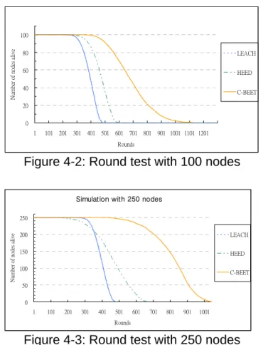
Figure 4-2: Round test with 100 nodes
Figure 4-3: Round test with 250 nodes
In figure 4-2 and 4-3, we showed the network lifetime under 100 nodes and 250 nodes. It is obvious that C-BEET can live longer time than HEED and LEACH. C-BEET is almost two times longer than LEACH and 1.33 times longer than HEED. LEACH uses random head selection without considering energy dispersion seriously so the first node dead time is earlier than HEED and C-BEET. Besides that, LEACH and HEED have to spend more energy than C-BEET while forming a cluster so it infers nodes in C-BEET can live longer.
We can observe that even we add the amount of nodes to 250, the network lifetime is not increased apparently but the first node dead time is delayed because there is more nodes can be selected as head so the energy cost is scattered. For HEED with 250 nodes, the slope of the curve is decreased that means HEED is good at dispersing the energy cost averagely to all the nodes in the field.
Simulation with 250 nodes
0 50 100 150 200 250 1 101 201 301 401 501 601 701 801 901 1001 Rounds N um ber of nodes al iv e LEACH HEED C-BEET 0 20 40 60 80 100 1 101 201 301 401 501 601 701 801 901 1001 1101 1201 Rounds N um ber o f node s al iv e LEACH HEED C-BEET
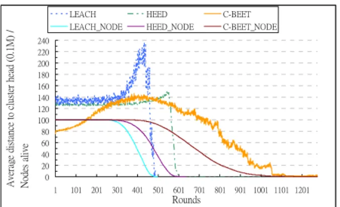
Figure 4-4: Average distance to cluster head with round test
Another factor that can influence the energy usage is the transmission distance while a node sends data to the cluster head. Figure 4-4 shows the variation of average distance to cluster head. We combined figure 4-2 into this figure. There are two parts in this graph, one is live nodes number and the other is average distance to cluster head. Let’s look at LEACH first, LEACH can keep the average distance at the beginning of the network but as soon as the nodes starts to die, the distance to cluster head increase quickly. Because of the long distance to the cluster heads, nodes in LEACH died quicker at the mid-end of the network. So the curve of live nodes suddenly dropped after the distance to cluster head increased.
The average distance to cluster head in HEED is very stable because the HEED algorithm defines a radius for each node to limit the range of cluster head advertisement. The curve only rises slightly at the end of the network. In C-BEET, the distance is small at beginning and after a time period, the weight of the nearest neighbors are getting higher so the nodes will choose a little farer nodes with less weight. This incurs the average distance to head increase to a stable value and till the network end. Generally, the average distance in C-BEET is less than LEACH and HEED at most of time. The transmission distance is the main factor that influence the energy cost. We combine the two types of curve so that can present a clear view of the relationship between network lifetime and average distance to cluster head.
0 20 40 60 80 100 120 140 160 180 200 220 240 1 101 201 301 401 501 601 701 801 901 1001 1101 1201 Rounds Av er ag e dis ta nc e to cl us te r he ad ( 0. 1M ) / N odes a live fs df sf df ds fs df ds fs df fs df sd ffff
LEACH HEED C-BEET
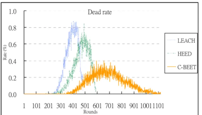
In figure 4-5, we present the “Dead rate” of the network. This graph shows the rate of dead node in each round. As we mentioned at the beginning of section 4, we simulated 500 times so the graph is the average value of the experiments. We can see that the peak of LEACH and HEED is higher than C-BEET, it means dead nodes in LEACH and HEED are separated into those rounds which the peak covered. The coverage of the network may be uncompleted because the nodes dead. The network coverage of wireless sensor network is very important because most applications hope that the sensor nodes can cover the field where they want to monitor. If there is somewhere uncovered, some data will be missed.
Unlike LEACH and HEED, the peak of C-BEET is wider so the nodes in C-BEET are dead slower and can keep the network coverage as long as possible. The result shows that the head selection algorithm in C-BEET is much better than other two schemes because C-BEET considers the residual energy seriously and avoids selecting the same node as cluster head frequently.
Figure 4-5: Dead rate of nodes Dead rate 0.0 0.2 0.4 0.6 0.8 1.0 1 101 201 301 401 501 601 701 801 901 10011101 Rounds Ra te (% ) LEACH HEED C-BEET
Initial energy (per node) protocol First node dies at (round) Last node dies at (round) C-BEET 196 506 HEED 133 315 0.25 J LEACH 121 259 C-BEET 401 1120 HEED 284 590 0.5 J LEACH 264 483 C-BEET 821 2140 HEED 610 1155 1 J LEACH 553 935
Table 4-2: The comparison of the protocols under different energy
Table 4-2 listed the performance of these schemes under different initial energy. In the former experiments, we set the initial energy to 0.5J per node. We compared to 0.25J and 1J per node here and discovered that the lifetime of the network is almost linearly related to the initial energy. So we can prolong the network lifetime by equip a higher capacity battery to the sensor nodes.
Scheme Node type Cluster construction overhead
Head Send: p N p N × − × + (1 ) 1 , receive: p N p N × − ×(1 ) LEACH
Member Send:1, receive: N*p at most
HEED All nodes N
p ⎥⎥+ × ⎤ ⎢ ⎢ ⎡ ) 1 1 log ( min 2
C-BEET All nodes Receive: 1
Table 4-3: The comparison of the construction overhead for each round
Table 4-3 provides the analysis of cluster construction overhead. The notation p refers to the probability to become a cluster head; N refers to the node number of the network. The analysis showed that in our scheme, sensor nodes only need to receive “Head Information” once. For
LEACH and HEED, nodes need to broadcast advertisement while cluster construction so the communication overhead is heavier than C-BEET.
4.3 Discussion
Section 4.2 showed the experiment results and they showed a great improvement on energy saving. We are going to discuss why C-BEET can save more energy than the other two schemes in two aspects.
In LEACH and HEED, nodes are self-organized. While forming nodes into clusters, nodes have no idea of geographic information of the network, that is to say, node decide itself to become a cluster head with no confidence if it is a good decision. There may have two head very closely to each other and obviously this is an unsuccessful cluster. Although HEED considered the radius of the cluster head advertisement message to control the cluster diameter, every node is still based on a probability to decide if it should become a cluster head. Depending on probability is not so stable for selecting the cluster heads.
But in C-BEET, nodes don’t have to deal with which one should become a cluster head. Instead of electing themselves, C-BEET computes how to cluster by base station for the nodes. That’s why we named our scheme with “centralized.” Base station has all the information of the network so it can compute an optimal solution for the current network. Figure 4-4 showed the material to support the statement.
The transmission distance is very important to the wireless sensor network. The RF module which is the component that consumes most energy in a sensor node. We have defined the power consumption model that is proportion to distance square. A good clustering can help sensor nodes to shorten their transmission distance to cluster heads. So that’s one of the aspects why C-BEET can save more energy than LEACH and HEED.
Another advantage brought by centralized architecture is no inter-cluster communication needed. LEACH and HEED pay huge energy cost while forming clusters. Head in LEACH has to broadcast advertisement first and then reply to each node which wants to join the cluster. LEACH lost lots of energy here and so does HEED. Nodes in C-BEET only need to wait the head information broadcasted from base station so there is no inter-cluster communication cost in C-BEET.
C-BEET performs better in terms of network lifetime and provides good energy dispersion so that can keep the network coverage (figure 4-5). The evaluation showed those and provided sufficient evidence to support those properties.
5. Conclusions
Power saving is one of the most challenging subjects in wireless sensor network. The mission of wireless sensor network is to sense data in the deployed field and of course we hope that the wireless sensor network can live as long as possible. The efficiency of power consumption makes huge influence on network lifetime. There are many researches on power saving in different aspects such as hardware architecture, operating system design, medium access control protocol, and application layer.
In this thesis, we research on how to transmit back data efficiently. We proposed a centralized energy efficient routing scheme for wireless sensor network. Unlike the traditional routing protocol for wireless sensor network, we use centralized architecture to achieve some properties that can help the sensor nodes save more energy. In the evaluation section, the experiment result showed that the properties we claimed is true and made great improvement in terms of network lifetime, transmission distance and energy dispersion.
6. Reference
[1] Wendi Rabiner Heinzelman, Anantha Chandrakasan, and Hari Balakrishnan, “Energy-Efficient Communication Protocol for Wireless Microsensor Networks,” In the Proceedings of the Hawaii International Conference on System Sciences, January 4-7, 2000, Maui, Hawaii
[2] Ossama Younis and Sonia Fahmy, “HEED: A Hybrid, Energy-Efficient, Distributed Clustering Approach for Ad-hoc Sensor Networks,” IEEE INFOCM 2004.
[3] Alice Wang and Anantha Chandrakasan, “Energy efficient system partitioning for distributed wireless sensor networks,” International Conference on Compilers, Architecture and Synthesis for Embedded Systems, Grenoble, France, 2002
[4] Seema Bandyopadhyay and Edward J. Coylek, “An ebergy efficient hierarchical clustering algorithm for wiesless sensor networks,” IEEE INFOCOM 2003.
[5] Fan Ye, Haiyun Luo, Jerry Cheng, Songwu Lu, Lixia Zhang, “A Two-Tier Data Dissemination Model for Largescale Wireless Sensor Networks,” ACM Mobicom 2002. [6] Jason Lester Hill, “System Architecture for Wireless Sensor Networks,” Master thesis of
U.C Berkeley. Spring 2003.
Proceedings of IEEE INFOCOM, April 2003
[8] C. R. Lin and M. Gerla, “Adaptive Clustering for Mobile Wireless Networks,” in IEEE J. Select. Areas Commun., September 1997.
[9] B. McDonald and T. Znati, “Design and Performance of a Distributed Dynamic Clustering Algorithm for Ad-Hoc Networks,” in Annual Simulation Symposium, 2001. [10] M. Gerla, T. J. Kwon, and G. Pei, “On Demand Routing in Large Ad Hoc Wireless
Networks with Passive Clustering,” in Proceeding of WCNC, 2000.
[11] S. Banerjee and S. Khuller, “A Clustering Scheme for Hierarchical Control in Multi-hop Wireless Networks,” in Proceedings of IEEE INFOCOM, April 2001.
[12] S. Basagni, “Distributed Clustering Algorithm for Ad-hoc Networks,” in International Symposium on Parallel Architectures, Algorithms, and Networks (I-SPAN), 1999.
[13] M. Chatterjee, S. K. Das, and D. Turgut, “WCA: A Weighted Clustering Algorithm for Mobile Ad Hoc Networks,” Cluster Computing, pp. 193–204, 2002.
[14] T. J. Kwon and M. Gerla, “Clustering with Power Control,” in Proceeding of MilCOM’99, 1999.
[15] A. D. Amis, R. Prakash, T. H. P. Vuong, and D. T. Huynh, “Max-Min D-Cluster Formation in Wireless Ad Hoc Networks,” in Proceedings of IEEE INFOCOM, March 2000.
[16] Ramgopal Reddy Mettu. “Approximation Algorithms for NP-Hard Clustering Problems.” PhD dissertation of University of Texas at Austin, 2002.
[17] Moses Charikar, Sudipto Guha, Eva Tardos, David B. Shmoys. “A constant-factor approximation algorithm for the k-median problem.” Journal of Computer and System Sciences, Volume 65, Issue 1, August 2002
[18] Vijay Arya, Naveen Garg, Rohit Khandekar and Adam Meyerson, “Local search heuristics for k-median and facility location,” Proceedings of 33rd ACM Symposium on Theory of Computing, Crete, Greece, 2001.
[19] Samdor P. Fekete, Joseph S. B. Mitchell and Karin Weinbrecht, “On the continuous Weber and k-median problems,” Proceedings of the 16th annual symposium on Computational geometry, Clear Water Bay, Kowloon, Hong Kong, 2000.
[20] Koen Langendoen and Niels Reijers, “Distributed localization in wireless sensor networks: a quantitative comparison,” The International Journal of Computer and Telecommunications Networking, Volume 43, Issue 4, November 2003
[21] Nirupama Bulusu, John Heidemann and Deborah Estrin, “GPS-less Low Cost Outdoor Localization for Very Small Devices,” IEEE Personal Communications, Special Issue on "Smart Spaces and Environments," Vol. 7, No. 5, pp. 28-34, October 2000.
[22] Lance Doherty, Kristofer S. J. Pister and Laurent El Ghaoui, “Convex Position Estimation in Wireless Sensor Networks,” In Proceedings of IEEE INFOCOM, volume 3, pages 1655-- 1663, Anchorage, Alaska, April 22-26 2001.
[23] Nissanka B. Priyantha, Anit Chakraborty, and Hari Balakrishnan, “The Cricket Location-Support System,” 6th ACM International Conference on Mobile Computing and Networking (ACM MOBICOM), Boston, MA, August 2000
[24] Jeffrey Hightower, Gaetano Borriello and Roy Want, “SpotON: An Indoor 3D Location Sensing Technology Based on RF Signal Strength,” UW CSE Technical Report #2000-02-02 February 18, 2000.
[25] Chris Savarese, “Robust Positioning Algorithms for Distributed Ad-Hoc Wireless Sensor Networks,” Proceedings of the General Track: 2002 USENIX Annual Technical Conference, pp. 317 – 327
[26] G. Pottie, “Wireless Sensor Networks,” Information Theory Workshop, June, 1998. [27] D. Estrin, R. Govindan, J. Heidemann, and S. Kumar, “Next Century Challenges:
Scalable Coordination in Sensor Networks,” Mobicom 1999
[28] G.J. Pottie and W.J. Kaiser, “Wireless Integrated Network Sensors,” Comm. of the ACM, vol. 43 No. 5, pp. 51-58, May 2000