以VIX指數偵測危機狀態之效果探討─TVTP方法之應用 - 政大學術集成

全文

(1)國立政治大學商學院金融學系碩士班碩士論文 Graduate Institute of Money and Banking National Chengchi University Master Thesis. 治政以 VIX 指數偵測危機狀態之效果探討─ 大立 ‧ 國. 學. TVTP 方法之應用. A Study of the Effects on Detecting Financial Crisis State Using. ‧. the VIX Index: Through the TVTP Approach. n. er. io. sit. y. Nat. al. Ch. engchi. i n U. v. 研究生：戴天君指導教授：陳威光博士. 中華民國一○二年六月.

(2) 謝辭回首論文撰寫，一路走來麻煩了許多人，點點滴滴早已刻骨銘心。師長的悉心教導，使初次做論文的我得以快速掌握問題並突破思考盲點，同時亦在待人處事、人際互動上給予我許多啟發。謝謝我的指導教授陳威光老師，從碩一以來就受老師許多照顧，輕鬆愉悅的學習環境讓我們既兼顧了學業、拓展了人脈、又能多元發展。謝謝林靖庭老師，多次扮演著協助學生打通任督二脈的關鍵角色。特別謝謝口試委員郭維裕老師、徐政義老師、婁天威老師的精闢指點，讓這篇論文更臻於完備。另外也謝謝郭維裕老師從我大學就讀國貿系時即不斷針砭砥礪，讓. 政治大論文路途漫長，夥伴們互相激勵，讓這段旅程不再孤單。謝謝芳儀，奇妙的立. 我在大學四年紮下堅實的學業基礎，而得以進入研究所殿堂學習。. ‧ 國. 學. 契機讓我們不論在何處都相互扶持，非常榮幸而且開心能在學生生涯的尾聲與妳結識。雅鈴、玠寬兩位好戰友，不論是學業或就業，很幸運每周都能向你們請益，. ‧. 更謝謝一直以來受到你們許多的幫助，有幸同門讓我收穫滿滿、不虛此行！謝謝. sit. y. Nat. 文彥提供我最重要的軟體讓論文得以完成，碩一常在課業、生活上麻煩你，與你. al. er. io. 聊天總是能吸收許多新知，真的既感激又開心。特別感謝國中好友政翰花了許多. v. n. 時間心力指導軟體操作，讓我能快速上手。而大學同窗祐汝二話不說地幫忙，以. Ch. engchi. i n U. 及持續關心與鼓勵，都令我備感溫馨。論文完稿之際，謝謝書婷、亭瑜義無反顧協助中英文潤稿，讓用字遣詞更精準；而幾次的相談，加上與仕成每周聚會聊天，成為我最重要的放鬆、充電時刻。口試前夕，謝謝好友宜欣的打氣；以及姿儀、深民在公車站貼心陪伴，這份感動永遠難忘。GPACer 們、于婷、宗儒、致遠、及金融所 100 級等好友們，謝謝你們這段期間的鼓勵，每句「加油」都令人感到窩心。最後，成長求學的歷程中，總是無怨無悔支持著我的父母，謝謝你們。. 戴天君謹誌民國一○二年六月.

(3) 摘要 2008 年全球爆發了金融海嘯，其後短短半年內，美國 S&P500 指數跌幅高達 48%，令金融市場投資人一片譁然，連帶造成各項投資工具的價格重挫，並正式確立了美國市場的空頭格局。在此同時，具有「投資人恐慌指標」之稱的波動度指數(VIX)卻上漲了 125%。VIX 指數在歷史上幾次重大國際金融危機發生時點皆呈現大幅彈升與劇烈波動的現象；相較之下，在市場穩定、多頭氣氛濃厚時， VIX 多處在低位且波動平緩。這兩種顯著差異的現象即 VIX 指數的狀態變化。本研究目的之一為判斷 VIX 指數是否隨著前述兩種市場多空情形，而在自. 政治大的方法為 Filardo 於 1994 立年發表的「時序變動型馬可夫轉換模型(TVTP)」。此外，. 身結構上發生相對應的變化，並試圖了解狀態間轉換的時間點為何。本研究採用. ‧ 國. 學. 本研究更同時從統計角度及各模型實際績效表現，來比較納入額外變數資訊的 TVTP 模型是否優於 Hamilton 於 1989 年所提出的不包含額外資訊的「固定轉移. ‧. 機率馬可夫轉換模型(FTP)」。最後，本研究亦將歸納有助於提升模型能力的變數，. sit. y. Nat. 以做為了解、甚至是判斷 VIX 指數變化的參考指標。. al. er. io. 實證發現 VIX 指數可依據 TVTP 模型而區分為「低平均、低波動」與「高. v. n. 平均、高波動」兩種結構，且確實反映金融市場處於「平靜」或「危機」的狀態。. Ch. engchi. i n U. 本文也發現納入特定變數的 TVTP 模型不僅在統計角度上顯著優於 FTP 模型，利用 TVTP 模型偵測出的狀態變化時點進行買賣操作得到的實際績效亦優於 FTP 模型。本研究同時也歸納出觀察 VIX 指數動態時最具參考性的三大指標─追蹤 S&P500 指數的 ETF 價格變化、10 年期信用價差和 5 年期信用價差，其中尤以 5 年期信用價差的模型在實際績效方面表現最佳，年化報酬率不僅優於 FTP 模型，亦超越同期大盤表現。. 關鍵字：波動度指數、金融危機、時序變動型馬可夫轉換模型、狀態轉換。 i.

(4) Abstract During the period from September, 2008 to March, 2009 after the financial crisis occurred, the S&P 500 index dropped about 48%, and global financial market suffered severe losses which established bear market firmly. Nevertheless, the “investor fear gauge”- CBOE Volatility Index rose 125% at the same time. Moreover, when some worldwide historic financial events or crises occurred, the VIX index also dramatically increased and fluctuated intensely. In contrast, while the market is tranquil or in a bull market, the level of VIX index keeps low and fluctuates smoothly;. 政治大 One of the purposes in this study is to identify state switching in VIX index, and 立. such structural change is called state switching.. the time-varying transition probability Markov switching model (TVTP) Filardo. ‧ 國. 學. developed in 1994 is used. Further, this paper investigates whether the effect of state. ‧. identification by TVTP model incorporating exogenous variables is better than FTP. sit. y. Nat. model which is without extra variables. Finally, this paper generalizes what variables. io. er. are beneficial for the model estimation and help observing VIX index. The empirical results indicate that the VIX index can truly be identified as two. n. al. states, and state switching. v i n C h exists. Moreover, indeed the engchi U. TVTP models which. incorporate respectively SPDR S&P500, 10-year credit spread, or 5-year credit spread are statistically significant better than the FTP model. Comparing all models through their practical performance, this paper finds six of nine TVTP models have higher return than FTP model, and even surpass the U.S. stock market index. Thus, this study concludes that the above three variables are the most significant useful indicators to observe the changes of VIX index, especially the 5-year credit spread.. Keywords: VIX, Financial Crisis, TVTP, State Switching. ii.

(5) Contents. 1. Introduction ................................................................................................................ 1 2. Literature Review....................................................................................................... 7 2.1 Ideas and Characteristics of VIX ..................................................................... 7 2.2 Variables for Predicting Financial Crisis and Economic Recession ................ 9 2.3 State Switching Issue and Application of Markov Switching Model ............ 18 3. Methodology ............................................................................................................ 22 3.1 Fixed Transition Probability (FTP) Model .................................................... 22 3.2 Time-varying Transition Probability (TVTP) Model ..................................... 23 3.3 Modification of TVTP Model in Practice ...................................................... 29 4. Empirical Results ..................................................................................................... 32 4.1 Data ................................................................................................................ 32 4.2 Process of Model Construction and Selection ............................................... 33. 立. 政治大. ‧. ‧ 國. 學. 4.3 Comparing TVTP Models with FTP Model in Practical Performance .......... 41 5. Conclusion ............................................................................................................... 48 References .................................................................................................................... 52 Appendix A: Estimated Parameters of Generalized TVTP Models ............................. 56 Appendix B: Details about Practical Performance Examination ................................. 60 Appendix C: Smoothed Probability Comparison ........................................................ 70. n. er. io. sit. y. Nat. al. Ch. engchi. iii. i n U. v.

(6) List of Tables. Table 1. Predictors in Jan Babecký et al. (2012) .......................................................... 11 Table 2. Summary of indicators ................................................................................... 15 Table 3. U.S. financial market variables using in this paper ........................................ 32 Table 4. Augmented Dickey Fuller Unit Root Test ..................................................... 34 Table 5. Significance test and SIC of models .............................................................. 35 Table 6. Significance test and SIC of models mixed with periods of lags ................... 37 Table 7. Significance test and SIC of models mixed with variables and lags.............. 38 Table 8. Estimates of state-dependent parameters of nine models .............................. 40 Table 9. Performance in return of each model ............................................................. 43. 立. 政治大. ‧. ‧ 國. 學. n. er. io. sit. y. Nat. al. Ch. engchi. iv. i n U. v.

(7) List of Figures. Figure 1. VIX index from 1990/1/2 to 2013/3/29 .......................................................... 2 Figure 2. Framework of research ................................................................................... 6 Figure 3. Changes of VIX index .................................................................................. 34 Figure 4. Smoothed probability of crisis state for various models .............................. 46. 立. 政治大. ‧. ‧ 國. 學. n. er. io. sit. y. Nat. al. Ch. engchi. v. i n U. v.

(8) 1. Introduction From 2004, the global financial markets have entered a relatively tranquil situation, and the market volatility measured by the volatility index derived from the S&P 500 index has been a lower level for a long time until 2007. But the S&P 500 index drops about 48% from September, 2008 to March, 2009. During the same period, the Chicago Board Options Exchange (CBOE) Volatility Index performs well and increases more than 125%. The negative correlation between the S&P 500 index and VIX index leads investors to explore the VIX as a way to protect their portfolios. 政治大. from market crash, and even invest in the derivatives from VIX index to earn excess. 立. return during the crisis periods.. ‧ 國. 學. VIX is known as the CBOE Volatility Index. It measures the implied volatility that is being priced based on the S&P 500 index options, and often mentioned as. ‧. “investor fear gauge”. The VIX offers an indication of the next 30-day implied. y. Nat. io. sit. volatility priced by a variety of options from the S&P 500 index option market. Thus,. n. al. er. VIX is an important sign of market expectations for near future volatility, and it is. i n U. v. commonly used to measure investor sentiment. It is important to understand that VIX. Ch. engchi. is forward-looking as it measures the volatility that investors expect to see in the market. Therefore, VIX is a successful market timing indicator (Hill and Rattray, 2004) and a useful tool for risk management because it is the benchmark for implied volatility of U.S. stock market. VIX is a successful signal for entering into or out of stocks. High value of VIX is interpreted to correspond to a more volatile market in the near future. When the macro-driven environment is not running well, investors expect the future returns will be low and the sentiment of investors become pessimistic. As a result, they start to sell off their stocks so that raising the market volatility and the VIX index will go high. 1.

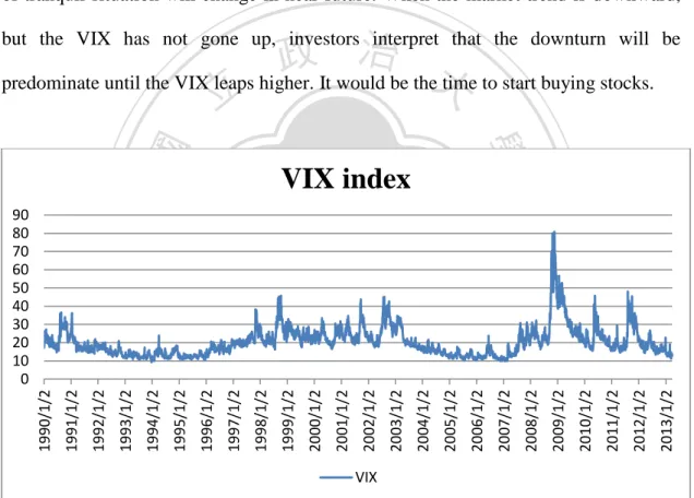
(9) VIX index can respond the atmosphere of the financial markets and show investors’ confidence level which implies both rational and irrational parts of their thinking. We should consider how the investors’ emotional aspect influences the volatility of financial markets so that we can make a better investment decision. Any trends or changes in the VIX index may help us evaluate the current and future situation of the market. For example, When VIX goes below 10 points, investors start selling stocks for short because they worry that the markets are being over-confident, and this kind of tranquil situation will change in near future. When the market trend is downward,. 政治大 predominate until the VIX leaps higher. It would be the time to start buying stocks. 立 VIX index. ‧ er. 2013/1/2. 2012/1/2. 2011/1/2. 2010/1/2. 2009/1/2. 2008/1/2. 2007/1/2. v. 2006/1/2. i n U 2005/1/2. 2003/1/2. 2002/1/2. 2001/1/2. 2000/1/2. engchi. 1999/1/2. Ch 1998/1/2. 1997/1/2. 1996/1/2. 1995/1/2. 1994/1/2. 1993/1/2. 1992/1/2. 1991/1/2. 1990/1/2. n. al. 2004/1/2. io. sit. y. Nat. 90 80 70 60 50 40 30 20 10 0. 學. ‧ 國. but the VIX has not gone up, investors interpret that the downturn will be. VIX Figure 1. VIX index from 1990/1/2 to 2013/3/29. Financial time series such as stock price or VIX index change dramatically especially in recent years. Figure 1 displays the daily VIX index from January, 1990 to March, 2013. Obviously, the VIX index is very volatile and sensitive to global financial market disturbances such as the Asian currency crisis in 1997, the Long-Term Capital Management (LTCM) crisis following the Russian financial crisis 2.

(10) in 1998, the 911 attacks in America, the 2002 Internet Bubble and the accounting scandals conducted by some U.S. large corporations, which made an enormous increase in VIX by 25% versus a huge decline in S&P 500 index about 36% (Fabozzi et al., 2006). In 2008, the Sub-prime crisis even caused the VIX reaching its highest level, 80.86, which is about 240% increase since January 2, 1990, and the S&P 500 index faced a substantial fall of about 48%. The European Sovereign debt crisis in 2010 made the VIX surge to 173% only in eight months and S&P 500 index decrease 12% at the same time. We can observe from the graph that generally VIX can be. 政治大 while the other is much fluctuated and have higher values. In this paper, I name the 立 viewed as two states (or regimes), one is relatively smoothed and in lower levels,. former one as “tranquility” state and the other as “crisis” state. This is consistent with. ‧ 國. 學. Connors (2002). For most investors, they are eager to identify the timing when the. ‧. two states occur, and especially, the state switching points between the two states. If. sit. y. Nat. investors know the switching moment, they can infer the future states and update their. io. er. investment decision.. Identifying the trend of a stock market in advance can help investors to gain. al. n. v i n excess return and avoid losses. C Of course, identifyingU h e n g c h i the trend of VIX index can also. achieve the same purpose. The most common classification of stock market regime is bull or bear market in the past literatures. The term bull market is associated with periods of upward trend in share prices and strong investment sentiment. On the contrary, the bear regime is the situation with downward trend in stock prices. In general, a bull regime is characterized with high returns and low volatility, and a bear regime is with low returns and very high volatility. We know that VIX index indicates the volatility of markets, thus, when the stock market is in the bull regime, the VIX index will stay in low levels and move smoothly. But when the bear market is coming, VIX will also respond to the dramatic change through the higher level of index and 3.

(11) intense volatility. Such structural break is regime shift or state switching. Regime shifts usually occur due to economic and financial crises. Once the crises happen, the single linear time series model commonly used before cannot identify the breaks in structure very well, the change in property of the financial time series motivate the use of regime switching models instead. Many studies have attempted to improve the predictability for financial market crises with macroeconomic and other variables. However, little research has explored the relationship between market turbulences and state switching. 政治大 To sum up, VIX index is very useful to show the financial market situation, 立. showed up in the VIX index through regime switching model.. especially during the periods of crisis or bear market. In other words, VIX can be. ‧ 國. 學. viewed as a downside risk indicator because it always obviously strongly responds to. ‧. the negative market sentiment when crises happen so that we can see from Figure 1. sit. y. Nat. that the level of VIX almost soars dramatically and the movement becomes very. io. er. volatile during the periods of financial crises or market instability. Therefore, this paper would like to clearly identify the state switching between tranquility and crisis. al. n. v i n state in the VIX index to helpCinvestors understandUthe current and future market hengchi condition and adjust their investment decision in advance so that they can increase their return and avoid suffering severe losses when the crises occur. This paper attempts to construct a model to understand the dynamics of VIX index and identify its state switching considering the influence of exogenous financial variables. The time-varying transition probability (TVTP) Markov state switching model which characterizes the unobservable tranquility or crisis states in VIX index and dynamics between them is applied. In addition to detect state shifts in the VIX index from the structural changes itself, most importantly, this paper investigates the role of U.S. financial market variables as leading indicators of state shifts in the VIX 4.

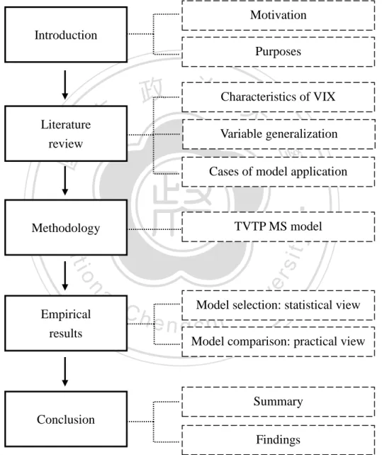
(12) index, and check whether these exogenous variables added into the model, such as interest rates or exchange rates, can better help us identify the state switching and the turning point between two states in the VIX index. Therefore, proving the effect of models with extra variables is better than the model without variables added, and generalizing what variables are beneficial for the model estimation and help observing VIX are very important purposes in this paper. The TVTP model is used to achieve above purposes, and this study also applies the likelihood ratio test (LR test) to check the statistically significance of the use of time-varying transition probability Markov. 政治大 model which is without the exogenous variables added. This paper also investigates 立. switching model compared with the fixed transition probability Markov switching. the practical performance of each model to double examine the TVTP models’ effect.. ‧ 國. 學. This paper is structured as follows. After the introduction in section 1, in section. ‧. 2 this paper reviews some literatures about basic idea of VIX and variables used to. sit. y. Nat. predict financial crisis, and learns how the past literatures apply the Markov state. io. er. switching model to financial time series data. Section 3 explains the methodology about two-state Markov switching model. Section 4 describes the preparation for the. al. n. v i n time series data using in modelCand presents the empirical h e n g c h i U results and discussion on. the results. Finally, Section 5 contains summary, findings, research limitations and future research suggestions. The framework of research is below. First, this paper describes the background of the VIX index applied in U.S. financial markets and understands the features of VIX when crisis occurs. Thus, this paper would like to explore further that whether the VIX index is really effective to detect the occurrence of crisis state, and which triggers motivation to study this issue. Then, through literature reviews, this paper generalizes some financial indicators which may be helpful to identify state switching in VIX index, and understand how the past literatures apply the methodology used in 5.

(13) this paper. Time-varying transition probability Markov regime switching model is the main methodology. This paper will incorporate the selected variables to construct TVTP models and test their significance statistically. And this paper will also compare their practical performance to examine their effectiveness when applying practically. Finally, conclusion and some findings in this paper will be summarized.. Motivation Introduction Purposes. 立. Variable generalization. ‧ 國. 學. Literature review. 政治 Characteristics 大 of VIX Cases of model application. ‧. TVTP MS model. n. al. er. io. sit. y. Nat. Methodology. Empirical results. Ch. i n U. v. Model selection: statistical view. engchi. Model comparison: practical view. Summary Conclusion Findings Figure 2. Framework of research. 6.

(14) 2. Literature Review 2.1 Ideas and Characteristics of VIX Whaley (1993) introduced the CBOE Volatility Index. It was known as “VXO” in the beginning, and constructed from the expected volatility priced in the contracts of eight at-the-money S&P 100 (OEX) put and call options. From September 22, 2003, CBOE estimated expected volatility with a new methodology, and it was called “VIX” since then. VIX calculates the expected volatility of S&P 500 index (SPX) by. 政治大 prices with a constant maturity of 30 days to expiration. The option price used to 立 averaging the weighted prices of SPX put and call options over a broad range of strike. estimate the VIX is the mid-point between the Bid/Ask spread of the options. ‧ 國. 學. including both at-the-money and out-of-the-money put and call options. In contrast,. sit. y. Nat. includes more information from wide range of option prices.. ‧. the old VXO caught just the volatility implied by at-the-money options. Thus, VIX. io. er. From the historical data, it is easy to observe that VIX index has an inverse relation with the stock market in term of prices. According to the CBOE’s statistic. al. n. v i n data, approximately 90% of theCtime the VIX index U h e n g c h i moved in an opposite direction with the S&P 500 index. Carr and Wu (2006) also find the existence of a negative. strong correlation between the changes in the VIX index and the performance of the S&P 500 index. When the market volatility is expected to increase, which is reflected in a high VIX, investors perceive the markets become more risky. Subsequently, they ask for higher rates of return on stocks, lowering the underlying stock prices. Conversely, when the market volatility is expected to decrease, which is implied by a low VIX, investors consider the market is less risky. They become more tolerant about the return rates, raising the stock prices. Whaley (2000) uses the weekly data from January, 1995 to December, 1999 to 7.

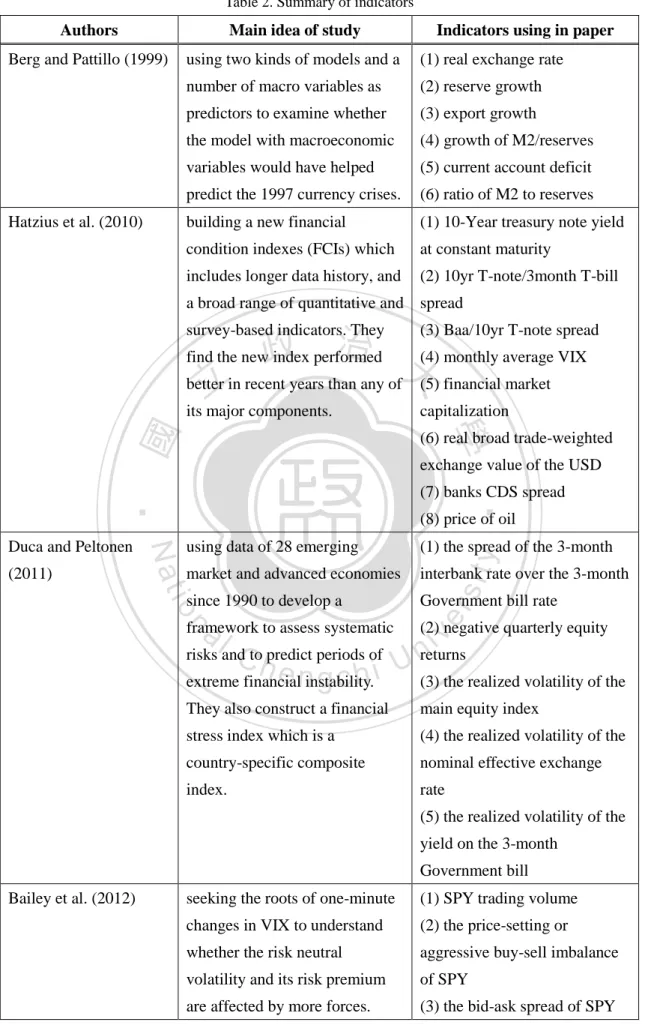
(15) study the negative relationship between the VIX index and S&P 100 index. He finds the asymmetric effect exists when market investors respond to the increase or decrease in the VIX index. He says that the degree which market treats the upward VIX index is more significant than the degree that market responds to the downward VIX. And high levels of VIX are coincident with high degrees of market turmoil, whether the turmoil is attributed to stock market decline or unexpected change in financial markets. In other words, the higher VIX means the greater fear. VIX changes much more dramatically during recessions than during booming. 政治大 negative, and extreme tail dependency between the VIX and the S&P 500 index return, 立 markets also shows the asymmetric movements. Sun and Wu (2009) find the strong,. and the negative dependency is asymmetric. Whaley (2008) indicates that if SPX. ‧ 國. 學. drops by 100 basis points, VIX will increase by 4.493%. On the other hand, if SPX. ‧. goes up by 100 basis points, VIX will only fall by 2.99%. Weng et al. (2011) reveal. sit. y. Nat. that this volatility index can only be utilized as a measure of market timing when it. io. er. gets to a definite and extreme level. The positive correlation between VIX and the future market returns is verified to be at the 5% significance level. However, this. al. n. v i n figure climbs as high as 36.47%C when the market is bearish h e n g c h i U and highly volatile.. Dueker (1997) points out that the volatility of financial assets usually exhibits. discrete shifts and mean reversion. Connors (2002) generalizes some reasons why VIX can work as a market signal. First, same as Dueker (1997), volatility has a long-term mean-reverting feature, which means periods of low volatility will be followed by periods of high volatility and vice-versa. When VIX begins mean reverting, it is accompanied by a market rally, whether upward or downward. Second, auto-correlation feature of volatility in short-term means if implied volatility rises today, the probability which implied volatility rises tomorrow is greater. Third, according to the dynamic feature of volatility, VIX reflects very recent market action. 8.

(16) Fourth, Connors has proved that VIX is able to tell when market top or bottom is.. 2.2 Variables for Predicting Financial Crisis and Economic Recession Next, this paper reviews some literatures about the issue of crisis prediction and generalizes the economic and financial indicators to identify macroeconomic condition, predict occurrence of crisis, or construct the earning warning systems. Berg and Pattillo (1999) use two kinds of models and a number of macro. 政治大 would have helped predict the 1997 currency crises. They have shown that the 立 variables as predictors to examine whether the model with macroeconomic variables. bilateral real exchange rate, reserve growth, export growth, growth of M2/ reserves,. ‧ 國. 學. current account deficit and ratio of M2 to reserves are important risk factors for the. ‧. prediction of currency crises.. sit. y. Nat. Hatzius et al. (2010) build a new financial condition indexes (FCIs) which. io. er. includes not only interest rates and asset prices with longer data periods, but a broad range of quantitative and survey-based indicators. Take some of total 45 indicators for. al. n. v i n example, 10-Year treasury noteC yield at constant maturity, h e n g c h i U 10yr T-note/3month T-bill. spread, Baa/10yr T-note spread, monthly average VIX, financial market capitalization, real broad trade-weighted exchange value of the USD, banks CDS spread, and price of oil are the components. They find the overall index performed better than any of its major components in recent years. Duca and Peltonen (2011) use quarterly data of 28 emerging market and advanced economies since 1990 to develop a framework to assess systematic risks and to predict periods of extreme financial instability. They test the ability of a wide range of composite indicators such as asset price (equity and property prices), credit (credit and monetary aggregates) and macro developments (GDP, inflation, 9.

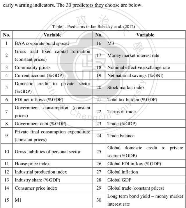
(17) government deficit, current account deficit). They also construct a financial stress index which is a country-specific composite index, and the five components are: (1) the spread of the 3-month interbank rate over the 3-month Government bill rate; (2) negative quarterly equity returns; (3) the realized volatility of the main equity index; (4) the realized volatility of the nominal effective exchange rate; (5) the realized volatility of the yield on the 3-month Government bill. They find that considering jointly various indicators in a multivariate framework and. 政治大 improves the performance of the models in forecasting systemic events. 立. taking into account jointly domestic and global macro-financial vulnerabilities greatly. Bailey et al. (2012) look for the factors of one-minute changes in VIX to. ‧ 國. 學. understand whether the risk neutral volatility and risk premium are affected by more. ‧. forces. They use the explanatory variables based on trade and quote information. sit. y. Nat. including SPY trading volume, the price-setting or aggressive buy-sell imbalance of. io. er. SPY, the bid-ask spread of SPY, trading volume of GLD, buy-sell imbalance of GLD, and changes in bid-ask spreads for the CDX NAIG index which reflects both. al. n. v i n corporate default risk and bondC market liquidity. They h e n g c h i Ufind that a significant portion. of VIX variability relates to trader behavior and macroeconomic fundamentals, so macroeconomic influences are significant. Temporary price effects are also observed around macroeconomic news releases. Soylemez (2012) tests for the relevant direction of Granger causality between the VIX index and S&P500 returns, and the results show that S&P500 influences VIX, but the opposite relationship does not exist. Jan Babecký et al. (2012) construct a dataset covering 36 developed countries from 1970 to 2010 at quarterly frequency to examine which potential leading indicators preceding economic crises are most useful in explaining the developed 10.

(18) economy’s real costs resulting from crises. They identified over 100 relevant macroeconomic and financial variables based on past studies and finally choose 30 variables as predictors. They find that about a third of the potential early warning indicators are useful for explaining the incidence of economic crises in EU and OECD countries in the past 40 years. The key early warning signal is growth in domestic credit to the private sector, while increase in government debt, the current account deficit, FDI inflow, or a fall in house prices and share prices could be considered late early warning indicators. The 30 predictors they choose are below.. 政治大. Table 1. Predictors in Jan Babecký et al. (2012). 立. No.. BAA corporate bond spread Gross total fixed capital formation (constant prices). Variable. 16. M3. 17. Money market interest rate. ‧. ‧ 國. 2. No.. 學. 1. Variable. Commodity prices. 18. Nominal effective exchange rate. 4. Current account (%GDP). 19. Net national savings (%GNI). 20. Stock market index. 21. Total tax burden (%GDP). 23. Trade (%GDP). 24. Trade balance. 8 9. FDI net inflows (%GDP). al consumption n. 7. Government prices). Government debt (%GDP). y. sit. (%GDP). io. 6. Domestic credit to private sector. er. 5. Nat. 3. v i n Ch 22 Terms of trade engchi U (constant. Private final consumption expenditure (constant prices). Global domestic credit to private. 10. Gross liabilities of personal sector. 25. 11. House price index. 26. Global FDI inflow (%GDP). 12. Industrial production index. 27. Global inflation. 13. Industry share (%GDP). 28. Global GDP. 14. Consumer price index. 29. Global trade (constant prices). 15. M1. 30. 11. sector (%GDP). Long term bond yield – money market interest rate.

(19) This paper also reviews some studies which apply the Markov regime switching model to identify the state switching in macroeconomic time series data. The origin and evolution of the model will be covered in the next part, but now this paper introduces some recent literatures about the application of Markov switching model first, especially focuses on the economic or financial variables using in these studies, and generalizes their influences to the models. Arias and Erlandsson (2005) propose an innovative early warning system of currency crises modeled by a time-varying Markov regime switching model applied. 政治大 to 2002 on a monthly basis, and the explanatory variables belonging to various 立 to six emerging South-East Asian countries. The sample covers the period from 1989. economic categories such as public deficit, central bank's credit to the public sector,. ‧ 國. 學. production growth, inflation, stock prices, banking fragility, trade balance deficit, the. ‧. real exchange rate, capital account, and 3-months LIBOR interest rate are chosen to. sit. y. Nat. enter the transition probability equation. The forecasting performance is satisfactory,. io. er. so they believe the time-varying transition probability Markov regime switching models are more adequate to build early warning systems of currency crises.. al. n. v i n C h macro variablesUwere useful in predicting bear Chen (2009) investigates whether engchi. markets, where bear market is defined as the regime with low return and high volatility of the S&P 500 price index. He focuses on the U.S. stock market and investigates the S&P 500 price index return from February, 1957 to December, 2007 using the monthly returns. Various macro variables include yield spreads (the difference between the 3-Month Treasury Bill Rate and the 10-Year Treasury Constant Maturity Rate, and the difference between the 3-Month Treasury Bill Rate and the 5-Year Treasury Constant Maturity Rate), inflation rates (consumer prices), money stocks (M1 and M2), aggregate output (industrial production), unemployment rates, federal funds rates, nominal effective exchange rates, and federal government 12.

(20) debts. He uses a modified version of the two-state Markov-switching model to examine empirically the cyclical variations in stock returns. Empirical evidence identifies there are two states in the S&P 500 stock index, the high-return stable and low-return volatile states in stock returns are conventionally labeled as bull markets and bear markets, respectively. He also finds term spreads and inflation rates are the most useful and significant predictors of recessions in the U.S. stock market. Mulvey and Zhao (2010) develop a dynamic approach to capture the critical market sentiments, with expected asset returns highly dependent on the associated. 政治大 economic factors within a regime-switching auto-regressive approach, including 立 economic regimes. Expected equity returns are characterized by a set of eight. changes in S&P 500 price index, changes in Treasury bond yields, changes in U.S.. ‧ 國. 學. dollar index, changes in implied volatility, changes in aggregate dividend yield, short. ‧. term interest rate, changes in treasury yield spread, and changes in credit spread. For. sit. y. Nat. constructing a portfolio with the Markov regime switching model, they employ. io. er. exchange traded funds to test the approach. Their findings are alternative regimes lead to differing correlation and return expectations over the designated asset classes, thus. al. n. v i n C hprovides much higher the developed investment portfolio returns with less risk than engchi U equity indices during the period of January 1999 to October 2010.. Baba and Sakurai (2011) use the Markov regime switching approach to investigate which macroeconomic variables can predict regime shifts in the VIX index. They choose the monthly VIX index as the dependent variable, and the following seven macroeconomic variables to test their influence on the switching probabilities from one regime to another: Consumer Price Index, Producer Price Index of finished goods, manufacturing capacity utilization, industrial production, the Federal funds rate, the difference between 5-year US government yield over 3-month Treasury bill rate (TERM 5Yt) and the difference between 10-year US government 13.

(21) yield over 3-month Treasury bill rate (TERM 10Yt). The two term spreads, TERM5Yt and TERM 10Yt, are found to have statistically significant positive coefficients in predicting the regime shifts from tranquil to turmoil regime. The likelihood ratio test also supports the models with each term spread have a significantly higher explanatory power compared with the baseline model without a macroeconomic variable. Engemann et al. (2011) consider whether oil price shocks significantly increase the probability that the economy enters recession in some industrialized countries.. 政治大 both net oil shocks and the term spread defined as the 10-year and 3-month Treasury 立 They adopt a Markov switching model in which the transition probabilities vary with. equivalents for each country to estimate the turning points. They find that oil shocks. ‧ 國. 學. indeed affect the probability that the economy transfers from expansion to recession. ‧. for most countries.. sit. y. Nat. To sum up, Mulvey and Zhao (2010) say that financial markets are usually. io. er. characterized as bullish or bearish, based on the economic indicators. It is observed that the equity market returns and volatility move in opposite directions more than. al. n. v i n 70% of the time. Credit spreadsC and yield spreads areU h e n g c h i generally wider in a downward. market than that in an upward market. Stock markets may stay in one state for some time before moving to another state at a later date. It is highly probable that market sentiment, market volatility, and the non-smooth asset return processes are state dependent. Therefore, ignoring such a possibility and information across the market regimes may cause incomplete investment strategies. A regime switching process is to characterize the sudden movements in market driven by the market information.. 14.

(22) Table 2. Summary of indicators. Authors. Main idea of study. Berg and Pattillo (1999). using two kinds of models and a. (1) real exchange rate. number of macro variables as. (2) reserve growth. predictors to examine whether. (3) export growth. the model with macroeconomic. (4) growth of M2/reserves. variables would have helped. (5) current account deficit. predict the 1997 currency crises.. (6) ratio of M2 to reserves. building a new financial. (1) 10-Year treasury note yield. condition indexes (FCIs) which. at constant maturity. includes longer data history, and. (2) 10yr T-note/3month T-bill. Hatzius et al. (2010). Indicators using in paper. a broad range of quantitative and spread (3) Baa/10yr T-note spread 治 find the new政 index performed (4) monthly average VIX 大 better in recent years than any of (5) financial market 立 its major components. capitalization survey-based indicators. They. ‧ 國. 學. (7) banks CDS spread. ‧. (8) price of oil (1) the spread of the 3-month. market and advanced economies. interbank rate over the 3-month. since 1990 to develop a. Government bill rate. n. Ch. risks and to predict periods of. engchi. extreme financial instability.. sit. io. al. framework to assess systematic. y. using data of 28 emerging. er. (2011). exchange value of the USD. Nat. Duca and Peltonen. (6) real broad trade-weighted. iv n returns U. (2) negative quarterly equity (3) the realized volatility of the. They also construct a financial. main equity index. stress index which is a. (4) the realized volatility of the. country-specific composite. nominal effective exchange. index.. rate (5) the realized volatility of the yield on the 3-month Government bill. Bailey et al. (2012). seeking the roots of one-minute. (1) SPY trading volume. changes in VIX to understand. (2) the price-setting or. whether the risk neutral. aggressive buy-sell imbalance. volatility and its risk premium. of SPY. are affected by more forces.. (3) the bid-ask spread of SPY. 15.

(23) They find a significant portion. (4) trading volume of GLD. of VIX variability relates to. (5) buy-sell imbalance of GLD. trader behavior and. (6) changes in bid-ask spreads. macroeconomic fundamentals.. for the CDX NAIG index. Jan Babecký et al.. constructing a dataset of 36. Quarterly frequency:. (2012). developed countries from 1970. See Table 1.. to 2010 to examine which potential leading indicators preceding economic crises are most useful in explaining the developed economy’s real costs resulting from crises. Monthly basis: 治政of currency 大(1) public deficit warning system crises modeled by a (2) central bank's credit to the 立 time-varying Markov regime public sector. Arias and Erlandsson. proposing an innovative early. 學. switching model applied to six. (3) production growth. emerging South-East Asian. (4) inflation. countries.. (5) stock prices. ‧. ‧ 國. (2005). (6) banking fragility. y. Nat. (7) trade balance deficit (9) capital account. Chen (2009). iv n Monthly returns: U. (10) 3-month LIBOR rate. n. al. er. io. sit. (8) the real exchange rate. Ch. investigating whether macro. engchi. variables were useful in. (1) 10-year yield spreads. predicting bear markets from. (2) 5-year yield spreads. February, 1957 to December,. (3) inflation rates. 2007. He uses the two-state. (4) M1 and M2. Markov-switching model to. (5) industrial production. examine empirically the cyclical. (6) unemployment rates. variations, and identifies there. (7) federal funds rates. are two states in the S&P 500. (8) nominal effective exchange. stock index.. rates (9) federal government debts. Mulvey and Zhao. developing a dynamic. (1) changes in S&P 500 price. (2010). systematic approach to capture. index. the critical market sentiments,. (2) changes in Treasury bond. 16.

(24) with expected asset returns. yields. highly dependent on the. (3) changes in U.S. dollar index. associated economic regimes.. (4) changes in implied volatility (5) changes in aggregate dividend yield (6) short term interest rate (7) changes in treasury yield spread (8) changes in credit spread. Baba and Sakurai. using the Markov regime. Monthly basis:. (2011). switching approach to. (1) Consumer Price Index. (2) Producer Price Index of 治政variables can 大finished goods macroeconomic predict regime shifts in the VIX (3) manufacturing capacity 立 index. The two term spreads are utilization. 學. found to have statistically. (4) industrial production. significant positive coefficients. (5) the Federal funds rate. in predicting the regime shifts. (6) the difference between. ‧. ‧ 國. investigate which. 5-year US government yield. y. Nat. over 3-month Treasury bill rate 10-year US government yield. Engemann et al. (2011). iv (1) net oil shocks n U. over 3-month Treasury bill rate. n. al. er. io. sit. (7) the difference between. Ch. considering whether oil price. engchi. shocks significantly increase the. (2) the term spread defined as. probability that the economy. the 10-year and 3-month. enters recession in some. Treasury equivalents. industrialized countries. They adopt a Markov switching model in which the transition probabilities vary to estimate the turning points.. 17.

(25) 2.3 State Switching Issue and Application of Markov Switching Model In this part, some literatures about the issue of state switching and the evolution of Markov switching model will be reviewed. Quandt (1958) begins time series modeling of regime shifts when he introduces the switching regression model. Goldfeld and Quandt (1973) extend the switching regression model and allow the regime shifts following Markov chain where the regime shifts is serially dependent. Their model is named Markov switching. 政治大 a similar approach but allows the regime shifts in dependent data and develops the 立. regression model. Based on Goldfeld and Quandt’s ideas, Hamilton (1989) establishes. Markov switching autoregressive model (MS-AR). In his model, the output mean. ‧ 國. 學. growth rate depends on whether the economy is in a phase of expansion or in a phase. ‧. of recession. He applies the technique to U.S. postwar data on real GNP. One possible. sit. y. Nat. outcome of maximum likelihood estimation of parameters might be the identification. io. er. of long-term trends in the U.S. economy, which separates periods with faster growth from those with slower growth. His statistical estimates of the economy's growth state. al. n. v i n C h of postwar recessions, is very consistent with NBER dating and might be used as an engchi U alternative way for assigning business cycle dates.. The application of Markov regime switching model in identifying the state switching starts from Turner et al. (1989). They capture the regime shifts behavior in stock market using MS-AR model, and their study highlights the usefulness of Markov switching model allowing state shifts to happen in mean and variance and fitting the data adequately. In Hamilton (1989)’s model, there is a discrete and unobservable variable named state variable or regime variable, which determines the state of the economy at each point of time. And the transition between states is governed by a constant-probability 18.

(26) process which is not influenced by other macroeconomic forces. Filardo (1994) extends the Markov-switching estimation method of Hamilton and incorporates the time-varying probabilities of transitions between the phases into Hamilton's model to examine differences in expansionary and contractionary phases of the business cycle. Filardo’s model is the time-varying transition probability Markov switching model (TVTP). The information variables he adds in the TVTP model as business-cycle predictors includes the Composite Index of Eleven Leading Indicators (CLI), the CLI's diffusion index, the Stock and Watson Experimental Index. 政治大 constant maturity treasury interest rate, the Standard and Poor's Composite Stock 立 of Seven Leading Indicators, the term premium which is the 10-year less the 1-year. Index, and the Federal Funds Rate. Using this technique and viewing monthly. ‧ 國. 學. industrial production as a proxy for aggregate output, he presents the statistical. ‧. significant empirical results that the output growth experiences one phase with a. sit. y. Nat. positive growth rate and another with a negative growth rate, and the former has. io. er. higher persistence. He also finds in the TVTP specification, the Composite Index of Eleven Leading Indicators performs well as an information variable for the business. n. al. Ch. cycle and turning points prediction.. engchi. i n U. v. Giot (2003) selects the time series data from January 3, 1992 to December 31, 2002 and uses a two-state Markov regime switching model applied to the observed daily VIX and VDAX implied volatility indices to find the volatility of both the U.S. S&P100 index and German DAX index switched from a low-value state to a high-value state around the events of the Asian financial crisis in 1997. From July 1997, the volatility pattern reverses itself as both indices stay almost continuously in the high-volatility state for the next five years due to the successive events such as the Russian crisis and the LTCM collapse, the fall of the NASDAQ, the start of the bear market in the U.S. and Europe and the terrorists’ attacks on September 11, 2001. 19.

(27) Moreover, market volatility has not reverted back to its initial low volatility state observed in the beginning of summer in 1997. He also shows that there has been a significant structural change in the asymmetric relationship between the stock index volatility and returns in both markets around the summer of 1997. Ismail and Isa (2008) used a univariate two-regime Markov switching autoregressive model (MS-AR) to capture regime shifts behavior in both the mean and the variance and the nonlinear feature existed in Malaysian stock market in four monthly stock market indices of Bursa Malaysia, which are the Composite Index, the. 政治大 MS-AR model is successful to capture the timing of regime shifts in the four indices 立. Industrial Index, the Financial Index and the Property index from 1974 to 2003. The. and these regime shifts occurred because of global economic and financial crises such. ‧ 國. 學. as the 1974 oil price shock, the 1987 stock market crash and the financial crisis in. ‧. 1997. Therefore, they concluded that major economic events happened around the. sit. y. Nat. world have influence on the behavior of Malaysia stock market returns. According to. io. er. the significant result of the likelihood ratio test, the use of nonlinear MS-AR(1) model is not only appropriate but rather superior to conventional linear AR(1) model.. al. n. v i n Wasim and Bandi (2011) C examine the regime switching behavior and seek for hengchi U. the existence of bull and bear regimes in the Indian stock market with daily data of. two leading Indian stock market indices: NSE-Nifty and BSE-Sensex from February 7, 1997 to December 11, 2010. They use a two state Markov switching autoregressive model and adopt the appropriate lag as AR(2), and it predicts that the Indian stock market has a very high probability to remain under bull regime compared to bear regime. The results also identify the bear phases during all major global economic crises including recent US sub-prime (2008) and European debt crisis (2010). Guo and Wohar (2006) examine multiple structural breaks in the mean level of market volatility measured by the VIX and VXO, and identify the dates of these mean 20.

(28) shifts. The data series for VIX are from 1990 to 2003 and for VXO are from 1986 to 2003. They find evidence which indicates three distinct periods existed in the evolution of volatility index, including a pre-1992 period, a period from 1992 to 1997, and a post-1997 period. The average volatility and its standard deviation were lowest during the period from 1992 to 1997, and the means of market volatility proxied by the VIX and VXO are not stable during the sample periods. Their findings provide statistical evidence consistent with the idea that the average level of market volatility changes infrequently but significantly over time.. 政治大 evolution of the VIX index that postulates the existence of two possible regimes: high 立. Romo (2012) presents a regime-switching framework to characterize the. volatility and low volatility, and assumes that the state variable governing the. ‧ 國. 學. transition between the two regimes follows a Markov process. The specification. ‧. accounts for deviations from normality due to the news about the economy or. sit. y. Nat. financial crisis, and exhibits persistent changes of the VIX index level.. io. er. To sum up, the issue about state switching in financial markets or economic business cycles motivates many researchers to study, and there are some literatures. al. n. v i n focusing on the state switching C in VIX index. Moreover, h e n g c h i U this paper finds that Markov switching model is a common methodology using to study the issue of state shift.. Nevertheless, little literatures investigate the effects of TVTP model on identifying state switching in the VIX index. Therefore, this paper will use the TVTP model and incorporate some appropriate indicators generalized from past literatures to study the dynamics of VIX index, and investigate whether the TVTP model can also perform well in identifying state shifts. Finally, generalizing some useful indicators to help understanding the changes of VIX index is one of the purposes in this paper.. 21.

(29) 3. Methodology In this section, this paper will introduce the regime switching model used in empirical process—Markov switching model. This paper will start from the model Hamilton developed in 1989, which is a fixed transition probability (FTP) Markov switching model. Then this paper will focus more detail on time-varying transition probability (TVTP) Markov switching model, which is extent from FTP and developed by Filardo in 1994. TVTP is also the main model in this paper.. 治政 3.1 Fixed Transition Probability (FTP) Model 大立 ‧ 國. 學. Hamilton (1989) studies regime shifts in dependent data and develops the Markov switching autoregressive model (MS-AR). The main feature of the regime. ‧. switching model is the possibility for some or all the parameters of the model to. sit. y. Nat. switch across different states (or regimes) according to a Markov process, which is. n. al. er. io. governed by a state variable, denoted 𝑆𝑡 . The model assumes that the state is an. i n U. v. unobservable stochastic process. Therefore, the state switching happens exogenously. Ch. engchi. with assigned probability to the occurrence of different states and this probability is called transition probability. The advantage of the transition probability is that it specifies a probability which regimes occur at each point of time rather than imposing particular dates at priori. Therefore, it allows the data to tell the nature and incidence of significant shifts. The MS-AR model can captures regime shifts in the mean, variance and also the parameter of the autoregressive process. A Markov switching autoregressive model of two states with an AR process of order p is given as follow:. 22.

(30) 𝑝. 𝑦𝑡 − 𝜇𝑆𝑡 = ∑ 𝜑𝑖 (𝑦𝑡−𝑖 − 𝜇𝑆(𝑡−𝑖) ) + 𝜖𝑡 𝑖=1. 𝜖𝑡 ~𝑁(0, 𝜎 2 ) 𝑆𝑡 = , 𝑆𝑡−𝑖 = ,. ,. P(𝑆𝑡 = |𝑆𝑡−1 = ) = 𝑝𝑖𝑗. Where 𝑆𝑡 and 𝑆𝑡−𝑖 are the unobserved regime variables that take the values of 1 or 2 and 𝑝𝑖𝑗 indicates the probability of switching from state j at time t-1 into state i at t.. 政治大 The transition probabilities between regimes are governed by a first order Markov 立. 學. P(𝑆𝑡 = |𝑆𝑡−1 = ) = 𝑝11. − 𝑝22. P(𝑆𝑡 = |𝑆𝑡−1 = ) = 𝑝21 =. − 𝑝11. y. Nat. P(𝑆𝑡 = |𝑆𝑡−1 = ) = 𝑝12 =. ‧. io. sit. P(𝑆𝑡 = |𝑆𝑡−1 = ) = 𝑝22. er. ‧ 國. process as follows:. n. a l𝑝11 + 𝑝21 = 𝑝22 + 𝑝12 = i v n Ch U engchi. Usually these probabilities are grouped together into the transition matrix, and they keep constant in the time series. I transfer the symbols and use p and q to represent the transition probabilities. 𝑝11 P = [𝑝. 21. 𝑝12 𝑞 𝑝22 ] = [ − 𝑞. −𝑝 ] 𝑝. 3.2 Time-varying Transition Probability (TVTP) Model I use the TVTP MS model Filardo (1994) developed as main methodology in this 23.

(31) paper, where the transition probabilities vary across time. Due to the asymmetric response to the bull and bear market in the volatility of VIX index I mentioned before, TVTP MS model can reveal this kind of characteristics. I distinguish VIX index into two states: tranquil and crisis, but both states are unobserved in advance. However, this unobserved binary state variable can pick up different phases of VIX index that corresponds to current state of tranquility or crisis. The evolution of the unobserved state measures the mean value and volatility of VIX index across the series, and will depend on available information represented in the time series of exogenous variables.. 政治大 conditions, but also some exogenous financial variables. Therefore, I implement the 立. In other words, the state of VIX index depends on not only the level of previous. time-varying transition probability (TVTP) Markov switching model as the main. ‧ 國. 學. methodology in this paper. This methodology allows for identification of not only. ‧. VIX index’s states, but also of financial variables which have statistically significant. sit. y. Nat. information about the changing of VIX.. io. er. First, I start from the introduction of basic idea of TVTP MS model. In this paper, I am interested in examining the characteristics of VIX index,. al. n. v i n C h MS model described , so I use the TVTP as below (see also Filardo engchi U. 𝑦𝑡 , = , , ,. and Gordon (1998)).. 𝑦𝑡 = 𝜇0 + ∑𝑝𝑖=1 𝜑𝑖 (𝐿)(𝑦𝑡−𝑖 − 𝜇𝑆(𝑡−𝑖) ) + 𝜖𝑡. if state 0. = 𝜇1 + ∑𝑝𝑖=1 𝜑𝑖 (𝐿)(𝑦𝑡−𝑖 − 𝜇𝑆(𝑡−𝑖) ) + 𝜖𝑡. if state 1. (1). Here 𝜑𝑖 (𝐿) = 𝛿1𝑖 + 𝛿2𝑖 𝐿 + ⋯ + 𝛿𝑑𝑖 𝐿𝑑−1 is a lag polynomial, 𝜖𝑡 ~𝑁(0, 𝜎 2 ), p is lag periods, and 𝑆𝑡. {0, }; thus the state-dependent mean is 𝜇𝑆𝑡 = 𝜇0 + 𝜇1 𝑆𝑡 . The state. variable 𝑆𝑡 is governed by a 2-state Markov-chain with transition probability matrix,. 24.

(32) P(𝑆𝑡 = 𝑠𝑡 |𝑆𝑡−1 = 𝑠𝑡−1 , 𝑋𝑡 ) = [. 𝑞(𝑋𝑡 ) − 𝑞(𝑋𝑡 ). − 𝑝(𝑋𝑡 ) ] 𝑝(𝑋𝑡 ). (2). Where the exogenous financial variables is 𝑋𝑡 = {𝑥𝑡, 𝑥𝑡−1 , … }. Compared with the transition matrix in FTP, it is obvious to observe that the transition probabilities in TVTP are the function of the exogenous financial driving covariates 𝑋𝑡 . The two states in this paper are named as tranquil state (state 0) and crisis state (state 1), respectively. Here I use 0 and 1 to replace the state 1 and 2 in the above part of FTP. Time-varying transition probabilities can gauge the persistence of the phases of. 政治大 vary with economic information 立 such as the financial driving covariates 𝑋 . The tranquil state and crisis state, and allow the probability of exiting a particular phase to 𝑡. ‧ 國. 學. variables I choose from the past literatures will input 𝑋𝑡 in the empirical process. The selection of functional form of 𝑞( ) and p( ) is typically probit or logistic type,. ‧. and I will use the probit type in this paper. Here 𝑞( ) and p( ) indicate the same. sit. y. Nat. meanings as used in the transition matrix in the above part of FTP. In TVTP model,. n. al. estimated. The conditional joint density distribution,. Ch. is: 1. engchi. er. io. the parameters in Eq.(1) and the transition probability parameters in Eq.(2) are jointly. i n U. v. , with AR dynamics of order r,. 1. (𝑦𝑡 |𝑦𝑡−1 , … , 𝑦𝑡− , 𝑋𝑡 ) = ∑ … ∑ ̂(𝑦𝑡 |𝑆𝑡 = 𝑠𝑡 , … , 𝑆𝑡− = 𝑠𝑡− , 𝑦𝑡−1 , … , 𝑦𝑡− ) =0. =0. × P(𝑆𝑡 = 𝑠𝑡 |𝑆𝑡−1 = 𝑠𝑡−1 , 𝑋𝑡 ) × P(𝑆𝑡−1 = 𝑠𝑡−1 , … , 𝑆𝑡− = 𝑠𝑡− |𝑦𝑡−1 , … , 𝑦𝑡− , 𝑋𝑡−1 ). (3). And the log-likelihood function is:. L(θ) = ∑𝑇𝑡=1 𝑙𝑛[. (𝑦𝑡 |𝑦𝑡−1 , … , 𝑦𝑡− , 𝑋𝑡 25. )]. (4).

(33) Here. denotes the parameter vector. The probability density function. (𝑦𝑡 |𝑦𝑡−1 , … , 𝑦𝑡− , 𝑋𝑡 ) makes a link with the exogenous variables contained in 𝑋𝑡 with regards to how they feature in the procedure for a Markov switching model for series 𝑦𝑡 via the transition probabilities. The information affects the system directly and indirectly through the inference of the past states. The information in 𝑦𝑡 and its lags directly affects the likelihood through the normal density, ̂, and the lags of 𝑦𝑡 indirectly. influence. the. likelihood. through. P(𝑆𝑡−1 = 𝑠𝑡−1 , … , 𝑆𝑡− = 𝑠𝑡− |𝑦𝑡−1 , … , 𝑦𝑡− , 𝑋𝑡−1 ) .. the. The. past. exogenous. states financial. variables directly affect the transition probabilities, P(𝑆𝑡 = 𝑠𝑡 |𝑆𝑡−1 = 𝑠𝑡−1 , 𝑋𝑡 ), and the distribution of the states,. 立. indirectly.. 政治大 P(𝑆 = 𝑠 ,…,𝑆 =𝑠 𝑡−1. 𝑡−1. 𝑡−. 𝑡−. |𝑦𝑡−1 , … , 𝑦𝑡− , 𝑋𝑡−1). ‧ 國. 學. Next, I would like to tell some details about calculating the transition probability.. ‧. In this paper, I use a latent variable version of probit model referring to Filardo. y. sit. io. n. al. P(𝑆𝑡 = ) = (𝑆𝑡. Ch. 0). P(𝑆𝑡 = 0) = (𝑆𝑡. 0) engchi U. er. time ,. Nat. and Gordon’s (1998) methodology to measure the transition probability matrix at each. v ni. (5). where 𝑆𝑡 is a latent variable defined by 𝑆𝑡 =. 0. +. 𝑥𝑡 + 𝑡 ~𝑁(0,. 𝑠𝑡−1 +. 𝑡. (6). ). The latent variable evolves due to a set of explaining variables, and Eq.(6) shows the relation between them. The standard normal distributional assumption will simplify the calculation of the transition probabilities. For instance, calculating transition probabilities at each time. is done by evaluating the conditional cumulative 26.

(34) distribution function for u. Let the function. |. ( (𝑥)) represent a conditional. standard normal cumulative distribution function (CDF) such that:. |. ̅( ) 1. ( (𝑥)) = ∫−. 1. (− 2. √2. 2. ). ~ (0, ). (7). Where ̅(𝑥) is the upper limit of the integration and is determined by Eq.(3) and (4). Therefore, 𝑝𝑡 and 𝑞𝑡 are: 𝑥 − )= − 政− − 治大 ( )= = 0) = − − 𝑥 立. 𝑝𝑡 = (𝑆𝑡 = |𝑆𝑡−1 = ) = (. 𝑡. 0. 𝑞𝑡 = (𝑆𝑡 = 0|𝑆𝑡−1. 𝑡. |. 𝑡. 0. 𝑡. |. (. (−. 0 0. −. −. 𝑥𝑡 − 𝑥𝑡 ). ) (8). ‧ 國. 學. In this model, the unobserved state variable, 𝑆𝑡 , is a nonlinear function of the. ‧. observable exogenous variables. The timing of those states is influenced through 𝑆𝑡. sit. y. Nat. by the vector of covariates, 𝑋𝑡 . The probit type model computes the probability that. n. al. er. io. the VIX index is in tranquil state or crisis state given a set of financial covariates, 𝑋𝑡 .. i n U. v. After the simple introduction of model construction, now I will move to the. Ch. engchi. method of parameter and state probability estimation.. Estimation is carried out via maximum likelihood (ML) methods. Once having the joint probability, I can calculate the likelihood estimates. The maximum likelihood estimates for. is obtained by maximizing the likelihood function by. updating the likelihood function at each iteration using the algorithm as follows. This is the log-likelihood function:. L(θ) = ∑𝑇𝑡=1 𝑙𝑛[ (𝑦𝑡 |𝑦𝑡−1 , … , 𝑦𝑡− , 𝑋𝑡. 27. )]. (9).

(35) And I rewrite the conditional probability density function as: (𝑦𝑡 |𝑦𝑡−1 , … , 𝑦𝑡− , 𝑋𝑡 ). (10). = ∑ (𝑦𝑡 |𝑆𝑡 = , 𝑦𝑡−1 , … , 𝑦𝑡− ) × P(𝑆𝑡 = |𝑦𝑡−1 , … , 𝑦𝑡− , 𝑋𝑡−1 ) 𝑖=1. = ∑ (𝑦𝑡 |𝑆𝑡 = , 𝑦𝑡−1 , … , 𝑦𝑡− ) ∑ 𝑝𝑖𝑗 P(𝑆𝑡−1 = |𝑦𝑡−1 , … , 𝑦𝑡− , 𝑋𝑡−1 ) 𝑖=1. 𝑗=1. Then I can calculate the filtered probability:. P(𝑆𝑡−1 = |𝑦𝑡−1 , … , 𝑦𝑡−. 立. 政治大 ,𝑋 ). (11). 𝑡−1. ‧. ‧ 國. 學. (𝑦𝑡−1 |𝑆𝑡−1 = , 𝑦𝑡−2 , … , 𝑦𝑡− ) × P(𝑆𝑡−1 = |𝑦𝑡−2 , … , 𝑦𝑡− , 𝑋𝑡−1) = ∑𝑖=1 (𝑦𝑡−1|𝑆𝑡−1 = , 𝑦𝑡−2 , … , 𝑦𝑡− ) × P(𝑆𝑡−1 = |𝑦𝑡−2 , … , 𝑦𝑡− , 𝑋𝑡−1 ). I can infer the filtered probability of each state through the above algorithm.. sit. y. Nat. Once estimating the model using the filtering algorithm, I can also make advanced. n. al. er. io. inference of the probability on the state using all the information from the beginning. i n U. v. to the end in the sample, and this kind of probability is called the smoothing. Ch. engchi. probability. The filtered and smoothing probabilities help us decide which state 𝑦𝑡 is at each point of time. Generally, in most applications, filtered probabilities and smoothing probabilities will give a very similar conclusion. (Ismail and Isa, 2008) Next, I would like to introduce the test of significance for TVTP models and the criterion of model selection in this paper. If there is no statistically meaningful information existed in the evolution of the state of the financial market contained in 𝑋𝑡 , the fixed transition probability (FTP) model is useful enough. In order to examine model’s effects, I will investigate the significance of the TVTP MS model using the likelihood ratio test (LR test). Formally, 28.

(36) under the null hypothesis of no time varying transition probabilities, the likelihood ratio test statistic is given by. ψ=. 2 × [𝐿( ) − 𝐿𝑅 ( )]~𝜒(𝑀 1 +𝑀2 ),𝛼. (12). where 𝐿𝑅 ( ) is the restricted log-likelihood, 𝑀1 + 𝑀2 is the number of restrictions on the test at significance level of 𝛼. LR test can be perceived as a test of the information of the exogenous financial variables in modeling and identifying the. 政治大 between alternative lag specifications for the conditioning variables. The Akaike 立. turning points in VIX index. Furthermore, the LR test can be implemented to select. information criterion (AIC) and the Schwartz information criterion (SIC) are usually. ‧ 國. 學. used to gauge the appropriate order of the lags of the variables in TVTP.. er. io. sit. y. ‧. Nat. 3.3 Modification of TVTP Model in Practice. In the empirical process, this paper will use the Matlab software to implement. al. n. v i n C h the model in U TVTP. For convenience when applying practice, this paper does not run engchi. the prototype MS model derived from Hamilton (1989) in the program directly;. instead, this paper uses the general form of the MS model. Therefore, changing the form of equation of Hamilton’s original model is necessary in order to match the form of the model used in program. The transferable process from Perlin (2012) is below. First, this paper combines Eq.(1) in previous part into a general form, and sets the periods of lag as 2, which means VIX index follows AR(2) process. The reason why setting AR(2) process for VIX is due to the results of statistic test, and details will be covered in next section. The core model in this paper is below, which is from Hamilton (1989). 29.

(37) 2. 𝑦𝑡 − 𝜇𝑆𝑡 = ∑ 𝜑𝑖 (𝑦𝑡−𝑖 − 𝜇𝑆(𝑡−𝑖) ) + 𝜖𝑡 𝑖=1. 𝜖𝑡 ~𝑁(0, 𝜎 2 ). From this equation, the independent variables are conditional on the states, an unobserved process. It means that the regressor ∑2𝑖=1 𝜑𝑖 (𝑦𝑡−𝑖 − 𝜇𝑆(𝑡−𝑖) ) is also unobserved prior to estimation. This paper will take a two-step estimation process to transfer the form of the model. Consider the following notation for Hamilton’s Model:. 立. 政治大 𝑧 =𝑦 −𝜇 𝑡. 𝑡. 𝑆𝑡. ‧ 國. 學. This is equivalent to:. ‧. 2. 𝑧𝑡 = ∑ 𝜑𝑖 𝑧𝑡−𝑖 + 𝜖𝑡. er. io. sit. y. Nat. 𝑖=1. Then rearrange those equations and get:. n. al. Ch. engchi. i n U. v. 𝑦𝑡 = 𝜇𝑆𝑡 + 𝑧𝑡. Where 𝑧𝑡 are the residuals from this reduced model. The two steps for the approximation which can be used to estimate Hamilton’s model are as follows. Step 1: Estimate using TVTP 𝑦𝑡 = 𝜇𝑆𝑡 + 𝜖𝑡 𝜖𝑡 ~𝑁(0, 𝜎 2 ) 𝑆𝑡 = 0, 30.

(38) Step 2: Retrieve the 𝜖̂𝑡 vector and regress it on two lags 2. 𝜖̂𝑡 = ∑ 𝛽𝑖 𝜖̂ 𝑡−𝑖 + 𝑣𝑡 𝑖=1 2 𝑣𝑡 ~𝑁(0, 𝜎𝑣𝑡 ). 2 the parameter 𝜎𝑣𝑡 from last equation will approximate 𝜎 2 of Hamilton’s model.. 立. 政治大. ‧. ‧ 國. 學. n. er. io. sit. y. Nat. al. Ch. engchi. 31. i n U. v.

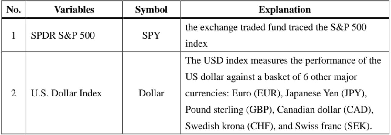
(39) 4. Empirical Results 4.1 Data This paper uses the daily VIX index as the time series data which is going to be identified as two states. And the following seven U.S. financial market variables generalized from past literatures are used to test their influence on the transition probabilities in TVTP MS model from one state to another. All of the data periods are from April 15, 2002 to March 29, 2013, and those daily data of the VIX index and the. 政治大 this paper finds the past literatures cover broad range of variables as the leading 立. financial variables are collected from Datastream. After reviewing many literatures,. indicators to predict financial crises, especially macroeconomic and financial. ‧ 國. 學. variables. But most of important macroeconomic variables data using in those studies. ‧. is seasonal or monthly frequency so that they cannot match the daily frequency of. sit. y. Nat. VIX index. VIX index has abundant and timely market information because of the. io. er. day-by-day trading activity, so this paper selects the seven financial variables which also have daily data instead of the macroeconomic variables which only have seasonal. al. n. v i n or monthly data to completely C match the daily VIXU h e n g c h i and try to decrease the loss of information. The seven financial variables are listed below.. Table 3. U.S. financial market variables using in this paper. No. 1. Variables SPDR S&P 500. Symbol SPY. Explanation the exchange traded fund traced the S&P 500 index The USD index measures the performance of the US dollar against a basket of 6 other major. 2. U.S. Dollar Index. Dollar. currencies: Euro (EUR), Japanese Yen (JPY), Pound sterling (GBP), Canadian dollar (CAD), Swedish krona (CHF), and Swiss franc (SEK). 32.

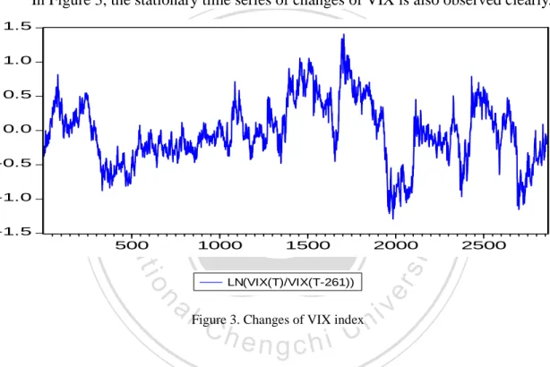
(40) A short-term debt obligation backed by the U.S.. 3. 3-month T-bill rate. T-bill. 4. 10-year term spread. Term10Y. 5. 5-year term spread. Term5Y. 6. 10-year credit spread. Credit10Y. 7. 5-year credit spread. Credit5Y. government with a maturity of 3 months the spread between 10-year Treasury bond yield and the 3-month T-bill rate the spread between 5-year Treasury bond yield and the 3-month T-bill rate the spread between 10-year BBB corporate bond yield and 10-year Treasury bond yield the spread between 5-year BBB corporate bond yield and 5-year Treasury bond yield. The VIX index, SPDR S&P 500 and Dollar index are calculated as ln where 𝑋𝑡. , 治政大 is the original index or price level of each variable at time t. The 立 261. ‧ 國. 學. transformation indicates that this paper focuses on the changes in these kinds of indexes or prices during the past one year. The other variables are measured in level.. ‧. In next part, the software-Eviews will be used to help analyzing the data, and the. n. al. er. io. sit. y. Nat. Matlab is used to estimate the TVTP MS model.. 4.2 Process of Model Construction and Selection. Ch. engchi. i n U. v. Before adopting the VIX index into the process of model estimation, this paper does the Augmented Dickey Fuller (ADF) Unit Root Test to check whether VIX index is a unit root series data. A time series data is not stationary when it has a unit root, and a non-stationary time series data will cause the consequence of spurious regression and ineffective inference if researchers don’t pay attention to the presence of unit root. From Table 4, it is significant to infer the VIX index (after calculation mentioned above) is stationary because it rejects the null hypothesis of unit roots existing. This paper also decides the lags of autoregression in the VIX index with 33.

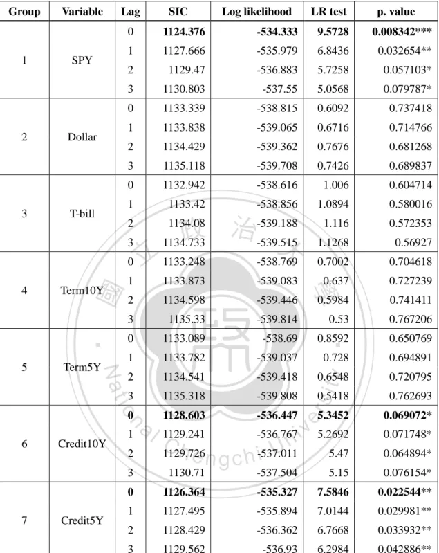
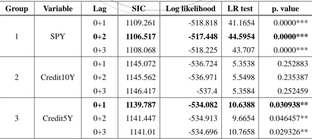
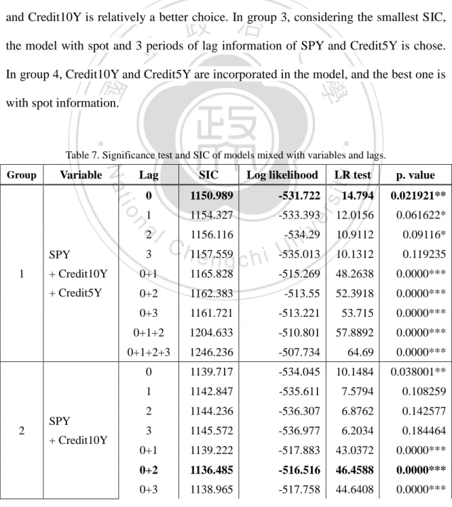
(41) Schwartz information criterion (SIC), and it suggests two periods of lag is the best.. Table 4. Augmented Dickey Fuller Unit Root Test. Method. Statistic. Prob.**. ADF - Fisher Chi-square. 17.1582. 0.0002. ADF - Choi Z-stat. -3.55639. 0.0002. In Figure 3, the stationary time series of changes of VIX is also observed clearly. 1.5 1.5. 1.0. 立. 1.0. 0.5. 政治大. 0.5. ‧ 國. 學. 0.0. 0.0. -0.5. ‧. -0.5. -1.0. 500. io. n. al. 1000 1500 2000 1000 1500 2000 2500 LN(VIX(T)/VIX(T-261)) LN(VIX(T)/VIX(T-261)). sit. -1.5 500. 2500. er. Nat. -1.5. y. -1.0. Ch. i n U. Figure 3. Changes of VIX index. engchi. v. Since the VIX index is stationary, the seven financial variables can be added into the TVTP model to examine whether the TVTP model incorporating exogenous information can significantly improve the fit of the data over FTP model which is without any exogenous variable. First, this paper adds the variables one by one, and calculates the SIC and likelihood ratio (LR) test statistics to estimate the significance of the TVTP model compared with the FTP model. In addition to the spot data, the lag data of each variable added into the TVTP model are from 1 to 3 periods, and this paper also examines the variation by turns. The estimated results are listed below. 34.

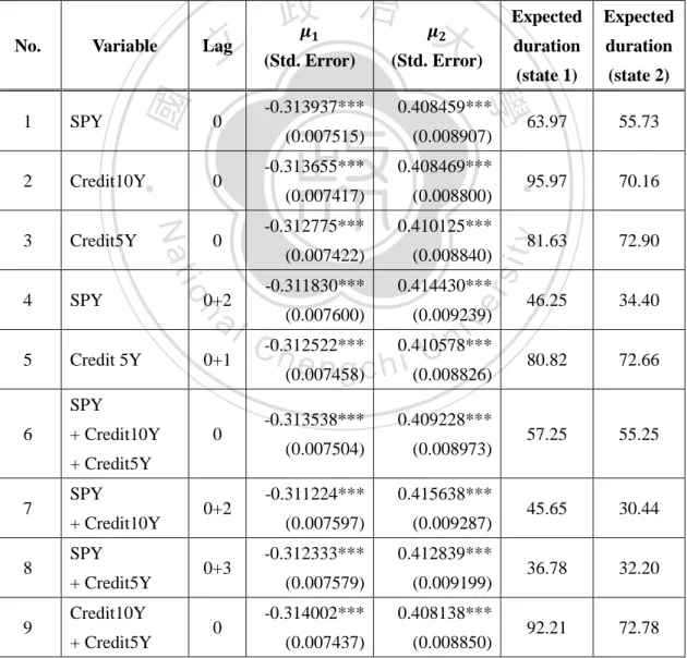
(42) Table 5. Significance test and SIC of models. 1. 2. 3. Variable. Lag. SPY. Dollar. T-bill. -534.333. 9.5728. 0.008342***. 1. 1127.666. -535.979. 6.8436. 0.032654**. 2. 1129.47. -536.883. 5.7258. 0.057103*. 3. 1130.803. -537.55. 5.0568. 0.079787*. 0. 1133.339. -538.815. 0.6092. 0.737418. 1. 1133.838. -539.065. 0.6716. 0.714766. 2. 1134.429. -539.362. 0.7676. 0.681268. 3. 1135.118. -539.708. 0.7426. 0.689837. 0. 1132.942. -538.616. 1.006. 0.604714. 1. 1133.42. -538.856. 1.0894. 0.580016. 1.116. 0.572353. 1.1268. 0.56927. 2. -539.188 治政 1134.733 -539.515 大. 0.7002. 0.704618. 1. 1133.873. -539.083. 0.637. 0.727239. 2. 1134.598. -539.446. 0.5984. 0.741411. 3. 1135.33. -539.814. 0.53. 0.767206. 0. 1133.089. -538.69. 0.8592. 1. 1133.782. -539.037. ‧. 0.650769. 0.728. 0.694891. 2. 1134.541. -539.418. y. 0.720795. 3. 1135.318. -539.808. 0.762693. 1128.603. -536.447. ‧ 國. -538.769. Term10Y. Term5Y. io. n. a 1 l. Credit10Y. 2. Credit5Y. 學. 立 1133.248. sit. 1134.08. 0. 3. 7. p. value. 1124.376. 0. 6. LR test. Nat. 5. Log likelihood. 0. 3. 4. SIC. 0.6548 0.5418. er. Group. 5.3452. 1129.241 -536.767 i v 5.2692 n C U h e n g c h -537.011 1129.726 5.47 i. 0.069072* 0.071748* 0.064894*. 1130.71. -537.504. 5.15. 0.076154*. 0. 1126.364. -535.327. 7.5846. 0.022544**. 1. 1127.495. -535.894. 7.0144. 0.029981**. 2. 1128.429. -536.362. 6.7668. 0.033932**. 3. 1129.562. -536.93. 6.2984. 0.042886**. Note: ***, ** and * indicate significance at 1%, 5% and 10% levels respectively.. The last columns indicate the significance for TVTP model compared with FTP model of each variable. This paper finds that the models respectively with variable SPY, Credit10Y, or Credit5Y are significant over all lag periods. It means that the 35.

(43) TVTP models with any one of the above three variables are statistically significant better than the FTP model which doesn’t incorporate any exogenous variable. Therefore, those three variables may be statistically useful to help distinguish the state switching in VIX index. Dollar, T-bill, Term10Y and Term5Y are not significant over all lag periods. In other words, these four variables may not be statistically helpful using in TVTP model to distinguish the state switching in VIX index. I also select the best specification by each model’s SIC among different periods of lag within every group. SIC is very useful to decide what period of lag is more appropriate for the. 政治大 the model specification than other periods of lags. For example, in the three 立. variable added in the model. Smaller SIC means the variable’s lag period is better for. significant groups of SPY, Credit10Y and Credit5Y, the SIC values of no lag models. ‧ 國. 學. are smaller than other models within the same groups respectively, therefore, this. ‧. paper infers that the models with spot information are more appropriate than others. io. er. 10-year credit spread or 5-year credit spread.. sit. y. Nat. with lagged information whether the exogenous information is from SPDR S&P500,. It makes sense that the information contained in the SPDR S&P500, 10-year. al. n. v i n C h is useful to identify credit spread and 5-year credit spread the structural breaks in VIX engchi U. index. I have mentioned in the previous sections that the S&P500 index is highly negatively correlated with the VIX index, and the empirical results of this paper also show that the SPDR S&P500 tracing and having a high correlation with the S&P500 index is helpful to identify the state switching in the VIX index. Thus, the result in this paper is consistent with past literatures. On the other hand, credit spread can indicate the atmosphere in the market or investors’ sentiment for the market condition. Because according to the credit spread definition used in this paper, when the market becomes instability, even recession, investors will worry that the default possibilities of BBB corporate bonds increase, so they ask higher yields to compensate the higher 36.