IEEE 802.16m 初始下行同步之數位訊號處理器實現

(1)

國立交通大學

電子工程學系電子研究所碩士班

碩

士

論

文

IEEE 802.16m 初始下行同步之數位訊號處理器實現

Digital Signal Processor Implementation of Initial Downlink

Synchronization for IEEE 802.16m

研究生：陳威宇

指導教授：林大衛博士

(2)

IEEE 802.16m 初始下行同步之數位訊號處理器實現

Digital Signal Processor Implementation of Initial Downlink

Synchronization for IEEE 802.16m

研究生: 陳威宇

Student: Wei-Yu Chen

指導教授: 林大衛博士 Advisor: Dr. David W. Lin

國立交通大學

電子工程學系電子研究所碩士班

碩士論文

A Thesis

Submitted to Department of Electronics Engineering & Institute of Electronics College of Electrical and Computer Engineering

National Chiao Tung University in Partial Fulfillment of the Requirements

for the Degree of Master of Science in

Electronics Engineering September 2011

Hsinchu, Taiwan, Republic of China

(3)

IEEE 802.16m 初始下行同步之數位訊號處理器實

現

研究生：陳威宇指導教授：林大衛博士

國立交通大學

電子工程學系電子研究所碩士班

摘要

本篇論文研究方向為針對 IEEE 802.16m 中初始下行同步裡，實作於數位訊號處理平台上的議題探討。當一個行動電話開始要進入網路的時候，我們必須與基地台做初始的同步。在初始的同步中，包含了符元時間偏移、載波偏移和前置符元序號(preamble index) 需要同步估測。我們利用前置符元的功率較一般資料符元(data symbol)大的特性做功率移動累加，藉由找到累加結果的峰值來估測前置符元的起始位置。由此起始位置向後推算一個符元長度以當作我們所估測出來的前置符元，而與真實的前置符元存在一個相位性錯誤(phase error)。我們利用此估測出來的前置符元推導其近似最大可能性估測(quasi maximum likelihood)以求得小數部分載波偏移和導出前置符元的通道估測的式子。我們在頻域上將此通道估測的式子經由估測出來的小數部分載波偏移補償之後，代入由合理範圍的整數部分載波偏移和不同的前置符元而得到的通道脈衝響應。再計算這些通道脈衝響應不同的精準符碼時間偏移序號64 點功率和並且選出最大的那一個，其所在的整數部分載波偏移、前置

(4)

接著，我們把此演算法實作於浮點運算與定點運算，以及比較兩者的效能。最後，把定點運算實現於數位訊號處理平台，並且最佳化我們的程式速度，減少運算複雜度，雖然定點運算會早成效能的衰減，但是結果依然可以接受。

(5)

Digital Signal Processor Implementation of

Initial Downlink Synchronization for IEEE

802.16m

Student：Wei-Yu Chen Advisor：Dr. David W. Lin

Department of Electronics Engineering

Institute of Electronics

National Chiao Tung University

Abstract

In this thesis, the research focus on initial downlink synchronization of IEEE 802.16m, and discuss the implementation issue of DSP.

When a mobile station entering to the network, it needs to perform initial synchronization, including of symbol timing offset, carrier frequency offset and preamble index. We utilize the trait which the power of preamble is larger than it of the common data symbol to compute the moving power sum, and then estimate the left boundary of preamble by finding out the peak value of moving power sum. A symbol period from this estimated boundary is regarded as the estimated preamble, which has a phase noise with the exact preamble. We derive the quasi maximum likelihood estimation from the likelihood function of the estimated preamble to obtain fractional carrier frequency offset (FCFO) and the formula of channel estimation. After compensating the estimated fractional carrier frequency offset to the formula of channel estimation, we substitute several reasonable integral carrier frequency offsets (ICFOs) and primary advanced preambles (PA-Preambles) into this formula and obtain channel impulse responses (CIRs). After that, we compute different fine timing offset index 64-points power sum of these CIRs and find out the peak value whose

(6)

the joint estimation.

In order to compare the performance, we implement the algorithm into the floating-point and fixed-point version. In the end, we modified the fixed-point version on the digital signal processor platform, and optimize the speed of our programs to reduce operation complexity. Although the performance is degraded because of fixed-point modification, the results still can be accepted.

(7)

誌謝

在交通大學裡度過的這兩年多來要感謝的人太多了，除了謝天以外，首先我想感謝林大衛老師，在這段時間以來的照顧以及在專業知識上給於了很多的幫助，如果沒有老師的話，也不能這麼順利的寫完這篇論文。老師同時教導了我很多做研究的方法及態度，讓我終身受用。接下來要感謝的是 CommLab 博班的學長，鴻志、彰哲、俊榮、伯森、世璞、朝雄，在課業或研究上也給予我多的幫助以及意見。有你們的幫助，讓我在碩班生涯中成長了很多，也學習到很多。再來要感謝的是曉盈、俊言、卓翰、智凱、強丹、郁婷、偵源、書瑋、兆軒、凱翔、峻利、復凱、婉瑜、怡茹、頌文以及學弟妹，在這段時間裡陪我吃喝玩樂，不管是課業上的討論還是聊天打屁，有你們的陪伴，讓我碩班生涯添加了很多色彩。最後要感謝的是我的家人以及馮捷，感謝一直來的支持與鼓勵，在我遇到挫折時包容我、體諒我，讓我在這段期間能夠無後顧之憂，完成這篇論文拿到碩士學位。本篇論文獻給所有曾經幫助過我的人，因為有你們，讓我成長茁壯，才能成就今天的我。陳威宇民國一○○年十月於風城‧新竹

(8)

List of Figures

2.1 Discrete-time model of the baseband OFDMA system (from [3]). . . 4

2.2 OFDMA symbol time structure (Fig. 478 in [5]). . . 5

2.3 Discrete-time baseband equivalent of an OFDMA system with M transmitting

users (from [4]). . . 6

2.4 OFDMA parameters (Table 794 in [5]). . . 10

2.5 More OFDMA parameters (Table 794 in [5]). . . 11

2.6 Basic frame structure for 5, 10 and 20 MHz channel bandwidths (Fig. 480

in [5]). . . 11

2.7 Definition of terms on the transmission chain (Fig. 479 in [5]). . . 12

2.8 Example of downlink physical structure (Fig. 499 in [5]). . . 13

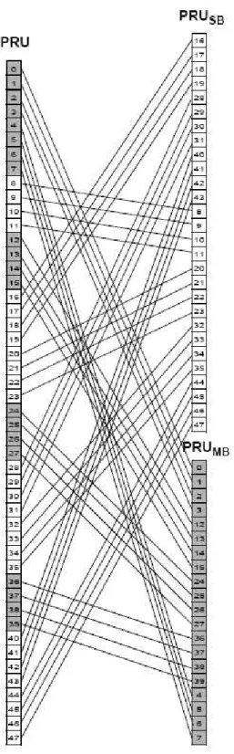
2.9 PRU to P RUSB and P RUM B mapping for BW = 10 MHz, KSB = 7 (Figure

500 in [5]). . . 18

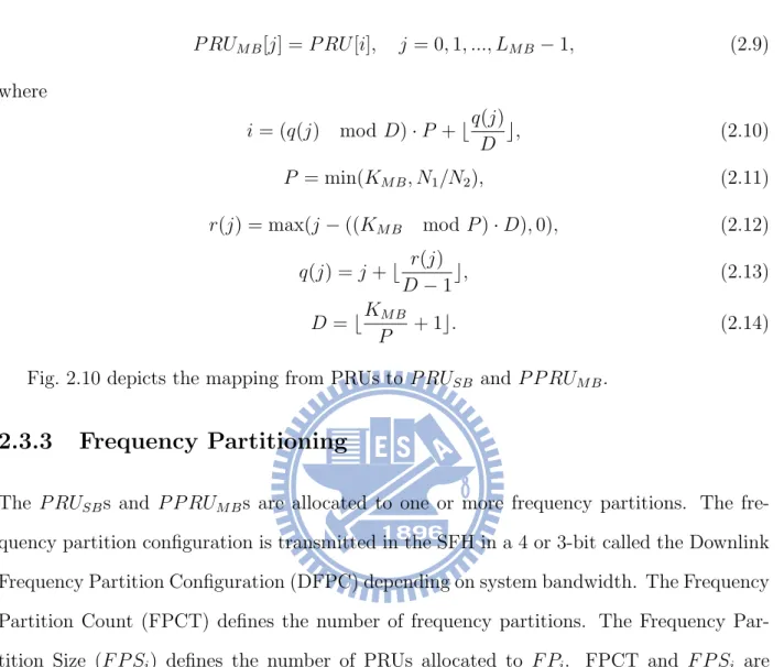
2.10 Mapping from PRUs to P RUSB and P P RUM B mapping for BW = 10 MHz

and KSB = 7 (Fig. 501 in [5]). . . 20

2.11 Location of the A-Preamble (re-arranged from Fig. 521 in [5]). . . 26

(13)

2.15 PA-Preamble Series (Table 815 in [5]). . . 28

2.16 SA-Preamble symbol structure of 5 MHz. . . 29

2.17 The allocation of sequence block for each FFT size (Fig. 524 in [5]). . . 30

2.18 SA-Preamble symbol structure for 512-FFT (Fig. 525 in [5]). . . 31

3.1 Window sliding structure [1]. . . 33

3.2 576 points power sum under AWGN in 0 dB [1]. . . 35

3.3 576 points power sum under SUI-5 at mobility 350 km/h in 0 dB [1]. . . 36

3.4 Channel impulse response of PB channel [1]. . . 37

3.5 Channel impulse response of SUI-5 channel [1]. . . 38

3.6 The estimated CIR with accurate ICFO, 8, compensating and correct PA-Preamble index, 1, under PB channel with 120 km/h, 0dB in SNR. . . 43

3.7 The CIR with the inaccurate ICFO, 6, compensating and incorrect PA-Preamble index, 0, under PB channel with 120 km/h, 0dB in SNR. . . 44

3.8 Block diagram of algorithm for initial DL synchronization [1]. . . 44

4.1 Functional block and CPU (DSP core) diagram [12]. . . 47

4.2 Code development cycle [14]. . . 51

4.3 Code development flow for C6000 (from [15]). . . 53

4.4 Software-pipelined loop (from [11]). . . 56

5.1 Block diagram of simulation procedure. . . 59

5.2 Histograms of coarse timing estimation under AWGN channel in different SNR. 60 5.3 Histograms of coarse timing estimation under SUI-1 channel in different SNR value for a velocity of 10 km/h. . . 61

(14)

5.4 Histograms of coarse timing estimation under SUI-1 channel in different SNR

value for a velocity of 90 km/h. . . 62

5.5 Histograms of coarse timing estimation under PB channel in different SNR

value for a velocity of km/h. . . 63

5.6 Histograms of coarse timing estimation under PB channel in different SNR

value for a velocity of 90 km/h. . . 64

5.7 Mean square error of FCFO estimation under SUI-1 and AWGN channels. . 65

5.8 Mean square error of FCFO estimation under SUI-3 and AWGN channels. . 66

5.9 Mean square error of FCFO estimation under PB and AWGN channels. . . . 67

5.10 Histograms of integer CFO estimation under AWGN channel in different SNR

values. . . 68

5.11 Histograms of integer CFO estimation under SUI-1 channel in different SNR

values at a velocity of 10 km/h. . . 69

5.12 Histograms of integer CFO estimation under SUI-1 channel in different SNR

values at a velocity of 90 km/h. . . 70

5.13 Histograms of PID detection under AWGN channel in different SNR values. 71

5.14 Histograms of PID detection under SUI-1 channel in different SNR values at

a velocity of 10 km/h. . . 72

5.15 Histograms of PID detection under SUI-1 channel in different SNR values at

a velocity of 90 km/h. . . 73

5.16 Histograms of fine timing estimation under AWGN channel in the different

SNR values. . . 74

(15)

5.18 Histograms of fine timing estimation under SUI-1 channel in different SNR

values at a velocity of is 90 km/h. . . 76

5.19 Histograms of fine timing estimation under PB channel in different SNR values at a velocity of 10 km/h. . . 77

5.20 Histograms of fine timing estimation under PB channel in different SNR values at a velocity of 90 km/h. . . 78

5.21 Fixed-point data formats used in DSP implementation. . . 80

5.22 Calculating the correlation in received PA-Preamble. . . 81

5.23 ICFO estimation and PID detection flow chart. . . 82

5.24 Histograms of coarse timing estimation under AWGN channel in different SNR values. . . 83

5.25 Histograms of coarse timing estimation under SUI-1 channel in different SNR values at a velocity of 10 km/h. . . 84

5.26 Histograms of coarse timing estimation under SUI-1 channel in different SNR values at a velocity of 90 km/h. . . 85

5.27 Histograms of coarse timing estimation under PB channel in different SNR values at a velocity of 10 km/h. . . 86

5.28 Histograms of coarse timing estimation under PB channel in different SNR values at a velocity of 90 km/h. . . 87

5.29 Mean square error of FCFO estimation under SUI-1 and AWGN channels with fixed-point and floating-point computation. . . 88

5.30 Mean square error of FCFO estimation under SUI-3 and AWGN channels with fixed-point and floating-point computation. . . 89

(16)

5.31 Mean square error of FCFO estimation under PB and AWGN channels with

fixed-point and floating-point computation. . . 90

5.32 Histograms of integer CFO estimation under AWGN channel in different SNR values with fixed-point implementation. . . 91

5.33 Histograms of integer CFO estimation under SUI-1 channel in different SNR values at a velocity of 10 km/h with fixed-point implementation. . . 92

5.34 Histograms of integer CFO estimation under SUI-1 channel in different SNR values at a velocity of 90 km/h with fixed-point implementation. . . 93

5.35 Histograms of PID detection estimation under AWGN channel in different SNR values with fixed-point implementation. . . 94

5.36 Histograms of PID detection under SUI-1 channel in different SNR values at a velocity of 10 km/h with fixed-point implementation. . . 95

5.37 Histograms of PID detection under SUI-1 channel in different SNR values at a velocity of 90 km/h with fixed-point implementation. . . 96

5.38 Summation of magnitude-squares for coarse timing estimation. . . 98

5.39 Assembly code of the coarse timing estimation (1/3). . . 101

5.40 Assembly code of the coarse timing estimation (2/3). . . 102

(17)

List of Tables

2.1 PRU Structure for Different Types of Subframes . . . 8

2.2 Mapping Between DSAC and KSB for 2048 FFT Size (Table 802 in [5]) . . . 15

2.3 Mapping Between DSAC and KSB for 1024 FFT Dize (Table 803 in [5]) . . . 16

2.4 Mapping Between DSAC and KSB for 512 FFT Size (Table 804 in [5]) . . . . 16

2.5 OFDMA Parameters for 2048 FFT When Tone Dropping Is Applied (Table 796 in [5]) . . . 17

2.6 OFDMA Parameters for 1024 FFT When Tone Dropping Is Applied (Table 796 in [5]) . . . 17

2.7 Mapping Between DFPC and Frequency Partition for 1024 FFT Size (Table 806 in [5]) . . . 21

4.1 Functional Units and Operations Performed [11] . . . 49

5.1 System Parameters Used in Our Study . . . 59

5.2 The error rate of timing estimation. . . 67

5.3 The error rate of timing estimation. . . 89

5.4 Coarse Timing Estimation Results for Optimization Level 3 . . . 97

5.5 Coarse Timing Estimation Results for Optimization Level 1 . . . 97

(18)

5.7 ICFO, PID, Fine Timing Estimation Results for Optimization Level 1 . . . . 99 5.8 DSP Optimization Results . . . 100

5.9 DSP Optimization Results with Inclusion and Exclusion of Memory Access 100

(19)

Chapter 1 Introduction

The IEEE 802.16m standard activity is a response to the ITU-R’s plan for the fourth-generation mobile communication standard IMT-Advanced, wherein it is specified that the data rate should be at least 100 Mbps in an environment with high mobility and 1 Gbps in a static environment. Since December 2006, the IEEE 802.16 standards group has set up the IEEE 802.16m (i.e., Advanced WiMAX or WiMAX 2) task group. The new frame structure developed by IEEE 802.16m is such that it can be compatible with IEEE 802.16e, reduce communication latency, support relay and coexist with other radio access techniques, so that it can become a promising candidates for 4G.

In this work, we study the digital signal processor (DSP) software implementation of a previously developed initial downlink synchronization method for IEEE 802.16m system with a time division duplex (TDD) mode [1,2]. The initial downlink synchronization involves frequency offset correction, timing recovery and bandwidth detection. In the procedure that we have developed, channel estimation is also obtained simultaneously.

Our DSP implementation uses Texas Instrument (TI) fixed-point DSP platform. We accelerate the execution speed of the programs and utilize difference optimization techniques to reduce the computational complexity.

This thesis is organized as follows. We first introduce the IEEE 802.16m standard in chapter 2. In chapter 3, we present the synchronization algorithm. Chapter 4 introduces

(20)

the DSP implementation platform. We discuss the DSP optimization methods and presents the optimization results in chapter 5. Finally, the conclusion is given in chapter 6, where we also point out some potential future work.

The contributions of this work are as follows:

• We modify the program from Matlab code to C code.

• We convert the code to fixed-point for implementation on DSP.

• We employ various optimization techniques to accelerate the execution speed of the

(21)

Chapter 2 Overview of the IEEE 802.16m

Standard

The IEEE 802.16m standard is based on orthogonal frequency division multiplexing (OFDM) and orthogonal frequency division multiple access (OFDMA). In this chapter, we introduce some basic concepts regarding OFDM and OFDMA first. Then we give an overview of the draft IEEE 802.16m standard. For simplicity, we only introduce the specifications that are most relevant to our study. For example channel coding, MAP messages, transmit diversity, etc., are ignored in this introduction.

2.1 Overview of OFDMA [3], [4]

OFDMA is considered one most appropriate scheme for future wireless systems, including 4G broadband wireless networks. In a typical OFDMA system, users may simultaneously transmit their data by modulating mutually exclusive sets of orthogonal subcarriers, so that their signal are separated in the frequency domain. One typical structure is subband OFDMA, where all available subcarriers are divided into a number of subbands and each user is allowed to use one or more subbands for the data transmission. Usually, pilot symbols are employed for the estimation of channel state information (CSI) within the subband. The IEEE 802.16m is one example of such systems. Figure 2.1 shows an uplink (UL) OFDMA system in which users simultaneously transmit to the base station (BS).

(22)

Figure 2.1: Discrete-time model of the baseband OFDMA system (from [3]).

2.1.1 Cyclic Prefix

Cyclic prefix (CP) or guard time is used in OFDM and OFDMA systems to overcome the intersymbol and intercarrier interference problems. The multiuser channel is usually substantially invariant within one-block (or one-OFDM(A)-symbol) duration. The channel delay spread plus symbol timing mismatch is usually smaller than the CP duration. In these conditions, users do not interfere with each other in the frequency domain when their signal are properly synchronized in frequency and in time.

A CP is a copy of the last part of the OFDM(A) symbol, as illustrated in Fig. 2.2. A

copy of the last Tg of the useful symbol period is used to collect multipaths from the preious

symbol to maintain the orthogonality among subcarriers. However, the transmitter energy increases with the length of the guard time while the receiver energy remains the same,

because the CP is discarded in the receiver. So there is a 10 log₁₀(1 − Tg/(Tb+ Tg)) dB loss

(23)

Figure 2.2: OFDMA symbol time structure (Fig. 478 in [5]).

2.1.2 Discrete-Time Baseband Equivalent System Model

The material in this subsection is mainly taken from [4]. Consider an OFDMA system with

M active users sharing a bandwidth of B =1

T Hz (where T is the sampling period) as shown

in Fig. 2.3. The system consists of K subcarriers of which Ku are useful subcarriers

(exclud-ing guard bands and DC subcarrier). The users are allocated non-overlapp(exclud-ing subcarriers according to their needs.

Let the discrete-time baseband channel consists of L multipath components as

h(l) =

L−1

X

m=0

hmδ(l − lm), (2.1)

where hm is a zero-mean complex Gaussian random variable with E[hih∗j] = 0 for i 6= j. In

the frequency domain,

H = Fh, (2.2)

where H = [H0, H1, ..., HK−1]T, h = [h0, ..., hL−1, 0, ..., 0]T and F is K-point discrete fourier

transform (DFT) matrix. The impulse response length lL−1 is upper bounded by the length

of CP (Lcp).

The received signal in the frequency domain is given by

Yn=

M

X

i=1

(24)

Figure 2.3: Discrete-time baseband equivalent of an OFDMA system with M transmitting users (from [4]).

where Xi,n = diag(Xi,n,0, ..., Xi,n,K−1) is K × K diagonal data matrix and Hi,n is the K × 1

channel vector H defined in (2.2) corresponding to the ith user in the nth symbol. The noise

vector Vn is distributed as CN (0, σ2IK).

2.2 Basic OFDMA Signal Structure in IEEE 802.16m

[5]

The Advanced Air Interface (AAI) defined by IEEE 802.16m is designed for nonline-of-sight (NLOS) operation in the licensed frequency bands below 6 GHz. The AAI supports time-division-duplexing (TDD) and frequency-time-division-duplexing (FDD) duplex modes, including

(25)

The AAI uses OFDMA as the multiple access scheme in both DL and UL. The material of this section is mainly taken from [5].

2.2.1 Resource Units

The OFDMA physical layer (PHY) of IEEE 802.16m organizer the subcarrier and OFDMA symbols into resource units as described below.

• Physical and logical resource units: A physical resource unit (PRU) is the basic physical

unit for resource allocation. It comprises Psc consecutive subcarriers by Nsym

consec-utive OFDMA symbols, where Psc = 18 and Nsym= 6 for type-1 subframes, Nsym= 7

for type-2 subframes, and Nsym = 5 for type-3 subframes. Table 2.2.1 illustrates the

PRU sizes for different subframe types. A logical resource unit (LRU) is the basic

logical unit for distributed and localized resource allocations. An LRU is Psc · Nsym

subcarriers for type-1, type-2, and type-3 subframes. The LRU includes the pilots that are used in a PRU. The effective number of data subcarriers in an LRU depends on the number of allocated pilots.

• Distributed resource unit: A distributed resource unit (DRU) contains a group of

sub-carriers which are spread across the distributed resource allocations within a frequency

partition. The size of DRU equals the size of PRU, i.e., Psc subcarriers by Nsym

OFDMA symbols.

• Contiguous resource unit: The localized resource unit, also known as contiguous

re-source unit (CRU), contains a group of subcarriers which are contiguous across the

localized resource allocations. The size of CRU equals the size of PRU, i.e., Psc

(26)

Table 2.1: PRU Structure for Different Types of Subframes Subframe Type Number of Subcarriers Number of Symbols

1 18 6

2 18 7

3 18 5

2.2.2 Basic Categories of Subcarrier

An OFDMA symbol is made up of subcarriers, the number of which determines the DFT size used. There are several subcarrier types:

• Data subcarriers: for data transmission.

• Pilot subcarriers: for various estimation purposes.

• Null subcarriers: no transmission at all, including subcarriers in the guard bands and

the DC subcarrier.

The purpose of the guard bands is to help enable proper bandlimiting.

2.2.3 Primitive Parameters and Derived Parameters

Four primitive parameters characterize the OFDMA symbols:

• BW : the nominal channel bandwidth.

• Nused: number of used subcarriers (which includes the DC subcarrier).

• n: sampling factor. This parameter, in conjunction with BW and Nused, determines

the subcarrier spacing and the useful symbol time. This value is given in Figs. 2.4 and 2.5 for each nominal bandwidth.

(27)

The following parameters are defined in terms of, i.e., derived from the primitive param-eters.

• NF F T: smallest power of two greater than Nused.

• Sampling frequency: Fs = bn · BW/8000c × 8000.

• Subcarrier spacing: 4f = Fs/NF F T.

• Useful symbol time: Tb = 1/4f .

• CP time: Tg = G × Tb.

• OFDMA symbol time: Ts= Tb+ Tg.

• Sampling time: Tb/NF F T.

2.2.4 Frame Structure

Fig. 2.6 illustrate the AAI basic frame structure. Each 20-ms superframe is divided into four 5-ms radio frames. When using the same OFDMA parameters as in Figs. 2.4 and 2.5 with channel bandwidth of 5, 10, or 20 MHz, each 5-ms radio frame further consists of eight subframes, when G = 1/8 and 1/16. With channel bandwidth of 8.75 or 7 MHz, each 5-ms radio frame further consists of seven and six subframes, respectively, for G = 1/8 and 1/16. In the case of G = 1/4, the number of subframes per frame is one less than that of other CP lengths for each bandwidth case. A subframe forms the unit of assignment for either DL or UL transmission. There are four types of subframes:

• Type-1 subframe consists of six OFDMA symbols.

• Type-2 subframe consists of seven OFDMA symbols.

(28)

Figure 2.4: OFDMA parameters (Table 794 in [5]).

• Type-4 subframe consists of nine OFDMA symbols. This type shall be applied only to

UL subframe for the 8.75 MHz channel bandwidth when supporting the WirelessMAN-OFDMA (i.e., IEEE 802.16e WirelessMAN-OFDMA) frames.

The basic frame structure is applied to FDD and TDD duplexing schemes, including H-FDD MS operation. The number of switching points in each radio frame in TDD systems shall be two, where a switching point is defined as a change of directionality, i.e., from DL to UL or from UL to DL.

(29)

Figure 2.5: More OFDMA parameters (Table 794 in [5]).

Figure 2.6: Basic frame structure for 5, 10 and 20 MHz channel bandwidths (Fig. 480 in [5]).

long TTI in FDD shall be 4 subframes for both DL and UL. The long TTI in TDD shall be the whole DL (UL) subframes for DL (UL) in a frame. Every superframe shall contain a superframe header (SFH). The SFH shall be located in the first DL subframe of the superframe and shall include broadcast channels.

(30)

Figure 2.7: Definition of terms on the transmission chain (Fig. 479 in [5]).

2.2.5 Transmitted Signal

The transmitted RF signal, as a function of time, during any OFDMA symbol to given by

s(t) = <{ej2πfc

(Nused−1)/2_X

k=−(Nused−1)/2,k6=0

ck· ej2π4f (t−Tg)} (2.4)

where

• t is the time, elapsed since the beginning of the OFDMA symbol, with 0 < t < Ts,

• ck is a complex number giving the QAM modulated value of the data to be transmitted

on the subcarrier whose frequency offset index is k, during the OFDMA symbol,

• Tg is the guard time,

• 4f is the subcarrier frequency spacing, and

• fc is the carrier frequency.

2.2.6 Transmission Chain

(31)

Figure 2.8: Example of downlink physical structure (Fig. 499 in [5]).

2.3 Downlink Transmission in IEEE 802.16m [5]

Again, this section is mainly taken from [5]. Each DL subframe is divided into 4 or fewer frequency partitions, each partition consisting of a set of PRUs across the total number of OFDMA symbols available in the subframe. Each frequency partition can include contiguous (localized) and/or non-contiguous (distributed) PRUs. Each frequency partition can be used for different purposes such as fractional frequency reuse (FFR) or multicast and broadcast services (MBS). Fig. 2.8 illustrates the DL physical structure in an example of two frequency partitions with frequency partition 2 including both contiguous and distributed resource allocations.

2.3.1 Subband Partitioning

The PRUs are first subdivided into subbands and minibands where a subband comprises

of N1 adjacent PRUs and a miniband comprises N2 adjacent PRUs, where N1 = 4 and N2

(32)

allocation of PRUs in frequency. Minibands are suitable for frequency diverse allocation and are permuted in frequency.

The number of subbands is denoted by KSB. The number of PRUs allocated to subbands

is denoted by LSB, where LSB = N1KSB. A 5, 4 or 3-bit field called Downlink Subband

Allocation Count (DSAC) determines the value of KSB depending on FFT size. The DSAC

is transmitted in the SFH. The remaining PRUs are allocated to minibands. The number of

minibands in an allocation is denoted by KM B. The number of PRUs allocated to minibands

is denoted by LMB, where LMB = N2KM B. The total number of PRUs is denoted as NPRU

where NP RU = LSB + LM B. The maximum number of subbands that can be formed is

denoted as Nsub where Nsub= bNP RU/N1c.

Tables 2.2 through 2.4 show the mapping between DSAC and KSB for FFT sizes of

2048, 1024, and 512, respectively. For system bandwidths in range of (10,20], the relation

between the system bandwidth and supported number of NP RU is listed in Table 2.5. The

mapping between DSAC and KSB is based on Table 2.2, the maximum valid value of KSB

is NP RU/4 − 3.

For those system bandwidths in range of (5,10], the relation between the system

band-width and supported number of NP RU is listed in Table 2.6. The mapping between DSAC

and KSB is based on Table 2.3, the maximum valid value of KSB is NP RU/4 − 2.

PRUs are partitioned and reordered into two groups called subband PRUs and miniband

PRUs and denoted P RUSB and P RUM B, respectively. The set P RUSB is numbered from 0

to LSB− 1, and the set P RUM B is numbered from 0 to LM B− 1. The mapping of PRUs to

P RUSB is given by

(33)

Table 2.2: Mapping Between DSAC and KSB for 2048 FFT Size (Table 802 in [5]) where i = N1·{{d Nsub Nsub− KSB e·bj + LMB N1 c+bbj + LM B N1 c·GCD(Nsub, d Nsub Nsub−KSBe) Nsub c} mod Nsub}+(j+LM B)·N1 (2.6) with GCD(x, y) being the greatest common divisor of x and y, and the mapping of PRUs

to P RUM B by

(34)

Table 2.3: Mapping Between DSAC and KSB for 1024 FFT Dize (Table 803 in [5])

Table 2.4: Mapping Between DSAC and KSB for 512 FFT Size (Table 804 in [5])

where i =     

N1· {d_N_subN_−Ksub_SB·e · b_Nk₁c + bb_Nk₁c ·

GCD(Nsub,d_Nsub−KSBNsub e)

Nsub c} mod Nsub

+(k) mod N1, KSB > 0,

i = k, KSB = 0.

(2.8)

Fig. 2.9 illustrates the PRU to P RUSB and P RUM B mappings for a 10 MHz bandwidth

(35)

Table 2.5: OFDMA Parameters for 2048 FFT When Tone Dropping Is Applied (Table 796 in [5])

Table 2.6: OFDMA Parameters for 1024 FFT When Tone Dropping Is Applied (Table 796 in [5])

2.3.2 Miniband Permutation

The miniband permutation maps the P RUM Bs to Permuted P RUM Bs (P P RUM Bs) to

(36)

Figure 2.9: PRU to P RUSB and P RUM B mapping for BW = 10 MHz, KSB = 7 (Figure 500

(37)

P RUM B to (P P RUM Bs) is given by P RUM B[j] = P RU[i], j = 0, 1, ..., LM B − 1, (2.9) where i = (q(j) mod D) · P + bq(j) D c, (2.10) P = min(KM B, N1/N2), (2.11) r(j) = max(j − ((KM B mod P ) · D), 0), (2.12) q(j) = j + b r(j) D − 1c, (2.13) D = bKM B P + 1c. (2.14)

Fig. 2.10 depicts the mapping from PRUs to P RUSB and P P RUM B.

2.3.3 Frequency Partitioning

The P RUSBs and P P RUM Bs are allocated to one or more frequency partitions. The

fre-quency partition configuration is transmitted in the SFH in a 4 or 3-bit called the Downlink Frequency Partition Configuration (DFPC) depending on system bandwidth. The Frequency Partition Count (FPCT) defines the number of frequency partitions. The Frequency

Par-tition Size (F P Si) defines the number of PRUs allocated to F Pi. FPCT and F P Si are

determined from DFPC as shown in Table 2.7. A field of 1, 2, or 3-bit parameter, called the Uplink Frequency Partition Subband Count (DFPSC), defines the number of subbands

allocated to frequency partition (F Pi), for i > 0. When UFPC = 0, DFPSC is equal to 0.

The number of subbands in ith frequency partition is denoted by KSB,F Pi. The number of

minibands is denoted by KM B,F Pi, which is determined by F P Si and and FPSC fields. The

number of subband PRUs and miniband PRUs in each frequency partition are LSB,F Pi =

N1· KSB,F Pi and LM B,F Pi = N2 · KM B,F Pi, respectively. We have KSB,F P i=

½

KSB, i = 0,

(38)

Figure 2.10: Mapping from PRUs to P RUSB and P P RUM B mapping for BW = 10 MHz

and KSB = 7 (Fig. 501 in [5]).

(39)

Table 2.7: Mapping Between DFPC and Frequency Partition for 1024 FFT Size (Table 806 in [5])

The mapping of subband PRUs and miniband PRUs to the frequency partition is given by

P RUF Pi(j) = ½ P RUSB(k1), 0 ≤ j < LSB,F Pi, P P RUM B(k2), LSB,F Pi ≤ j < (LSB,F Pi + LM B,F Pi), (2.17) where k1 = i−1 X m=0 LSB,F Pm + j (2.18) and k2 = i−1 X m=0 LSB,F Pm + j − LSB,F Pi. (2.19)

2.4 Cell-Specific Resource Mapping [5]

The content of this section is mainly taken from [5]. P RUF P is are mapped to LRUs. All

further PRU and subcarrier permutations are constrained to the PRUs of a frequency par-tition.

(40)

2.4.1 CRU/DRU Allocation

The partition between CRUs and DRUs is done on a sector specific basis. A 4 or 3-bit

Downlink subband-based CRU Allocation Size (DCASSBi) field is sent in the SFH for each

allocated frequency partition. DCASSBi indicates the number of allocated CRUs for

parti-tion F Pi in unit of subband size. A 5, 4 or 3-bit Downlink miniband-based CRU Allocation

Size (DCASM B) is sent in the SFH only for partition F P0 depending on system bandwidth,

which indicates the number of allocated miniband-based CRUs for partition F P0. The

num-ber of CRUs in each frequency partition is denoted LCRU,F P i, where

LCRU,F P i =

½

CASSBi· N1+ CASM B · N2, i = 0,

CASSBi· N1, 0 < i < FPSC. (2.20)

The number of DRUs in each frequency partition is denoted LDRU.F P i, where LDRU,F P i =

F P Si− LCRU,F P i for 0 ≤ i < FPSC and F P Si is the number of PRUs allocated to F Pi. The

mapping of P RUF P i to CRUF P i is given by

CRUF P i[j] =

½

P RUF P i[j], 0 ≤ j < CASSBi· N1, 0 ≤ i < FPSC,

P RUF P i[k + CASSBi· N1], CASSBi· N1 ≤ j < LCRU,F P i, 0 ≤ i < FPSC,

(2.21)

where k = s[j − CASSBi· N1], with s[ ] being the CRU/DRU allocation sequence defined as

s[j] = {P ermSeq(j) + DL P ermBase} mod {F P Si− CASSBi· N1}. (2.22)

where P ermSeq() is the permutation sequence of length (F P Si − CASSBi · N1) and is

determined by SEED = IDcell · 343 mod 210_{, DL P ermBase is an interger ranging from 0}

to 31, which is set to preamble IDcell. The mapping of P RUF P i to DRUF P i is given by

DRUF P i[j] = P RUF P i[k + CASSBi· N1], 0 ≤ j < LDRU,F P i. (2.23)

(41)

remain-2.4.2

Subcarrier Permutation

The subcarrier permutation defined for the DL distributed resource allocations within a frequency partition spreads the subcarriers of the DRU across the whole distributed resource allocations. The granularity of the subcarrier permutation is equal to a pair of subcarriers.

After mapping all pilots, the remainder of the used subcarriers are used to define the distributed LRUs. To allocate the LRUs, the remaining subcarriers are paired into contiguous tone-pairs. Each LRU consists of a group of tone-pairs.

Let LSC,l denote the number of data subcarriers in lth OFDMA symbol within a PRU,

i.e., LSC,l = PSC − Nl, where nl denotes the number of pilot subcarriers in the lth OFDMA

symbol within a PRU. Let LSP,l denote the number of data subcarrier-pairs in the lth

OFDMA symbol within a PRU and is equal to LSC,l/2. A permutation sequence P ermSeq()

performs the DL subcarrier permutation as follows. For each lth OFDMA symbol in the subframe:

1. Allocate the nl pilots within each DRU as described in [5] Section (16.3.4.4). Denote

the data subcarriers of DRUF P i[j] in the lth OFDMA symbol as

SCF P i

DRU,j,l[k], 0 ≤ j < LDRU,F P i, 0 ≤ k < LSC,l. (2.24)

2. Renumber the LDRU,F P i · LSC,l data subcarriers of the DRUs in order, from 0 to

LDRU,F P i · LSC,l − 1. Group these contiguous and logically renumbered subcarriers

into LDRU,F P i · LSP,l pairs and renumber them from 0 to LDRU,F P i · LSP,l − 1. The

renumbered subcarrier pairs in the lth OFDMA symbol are denoted as

RSPF P i,l[u] = {SCDRU j,lF P i [2v], SCDRU j,lF P i [2v + 1]}, 0 ≤ u < LDRU,F P iLSP,l, (2.25)

where j = bu/LSP,lc and v = {u} mod (LSP,l).

(42)

LRU, s = 0, 1, . . . , LDRU,F P i− 1, where the subcarrier permutation formula is given by SCF P i LRU s,l[m] = RSPF P i,l[k], 0 ≤ m ≤ LSP,l, (2.26) with k = LDRU,F P i· f (m, s) + g(P ermSeq(), s, m, l, t). (2.27) In the above, 1. SCF P i

LRU s,l[m] is the mth subcarrier pair in the lth OFDMA symbol in the sth distributed

LRU of the tth subframe;

2. m is the subcarrier pair index, 0 ≤ m ≤ LSP,l− 1;

3. l is the OFDMA symbol index, 0 ≤ l ≤ Nsym− 1;

4. s is the distributed LRU index, 0 ≤ s ≤ LDRU,F P i− 1;

5. t is the subframe index with respect to the frame;

6. P ermSeq() is the permutation sequence of length LDRU,F P i and is determined by

SEED = IDcell · 343 mod 210_;

7. g(P ermSeq(), s, m, l, t) is a function with value in the range [0, LDRU,F P i − 1], which

is defined according to

g(P ermSeq(), s, m, l, t) = {P ermSeq[{f (m, s) + s + l} mod {LDRU,F P i}]

+DL P ermBase} mod LDRU,F P i. (2.28)

where DL P ermBase is set to preamble IDcell; and

(43)

2.4.3 Random Sequence Generation

The permutation sequence generation algorithm with 10-bit SEED (Sn−10, Sn−9, ..., Sn−1)

shall generate a permutation sequence of size M according to the following process:

• Initialization

1. Initialize the variables of the first order polynomial equation with the 10-bit seed,

SEED. Set d1 = bSEED/25c + 1 and d2 = SEED mod 25.

2. Initialize the maximum iteration number, N = 4.

3. Initialize an array A with size M to contents 0, 1, . . . , M − 1 (i.e., A[i] = i, for 0 ≤ i < M ).

4. Initialize the counter i to M − 1. 5. Initialize x to −1.

• Repeat the following steps if i > 0

1. Initialize the counter j to 0. 2. Loop as follows:

(a) Increment x and j by 1.

(b) Calculate the output variable of y = {(d1· x + d2) mod 1031} mod M.

(c) Repeat the above steps (a) and (b), if y ≤ i and j < N . (d) If y ≤ i, set y = y mod i.

(e) Swap the ith and the yth elements in the array, i.e., perform the steps T emp =

A[i], A[i] = A[y], and A[y] = T emp.

(f) Decrement i by 1.

(44)

SU0

SU1

SU2

Superframe : 20ms

F0

F1

F2

F3

TDD frame : 5ms

Superframe Header PA-Preamble SA-Preamble

DL SF DL SF DL SF UL SF UL SF TTG RTG

Figure 2.11: Location of the A-Preamble (re-arranged from Fig. 521 in [5]).

2.5 Advanced Preamble (A-Preamble) Structure [5]

The material in this subsection is mainly taken from [5]. There are two types of Ad-vanced Preamble (A-Preamble): primary adAd-vanced preamble (PA-Preamble) and secondary advanced preamble (SA-Preamble). One PA-Preamble symbol and three SA-Preamble sym-bols exist within the superframe. The location of an A-Preamble symbol the first symbol of a frame. PA-Preamble is at the first symbol of second frame in a superframe while SA-Preamble is at the first symbol of each of the remaining three frames. Fig. 2.11 depicts the location of A-Preamble symbols.

(45)

Figure 2.12: PA-Preamble symbol structure of 5-MHz system (Fig. 522 in [5]). 297 299 301 509 511 513 515 723 725 727 …… _…… DC 297 299 301 509 511 513 515 723 725 727 …… _…… DC

Figure 2.13: PA-Preamble symbol structure of 10 MHz system [1].

configuration.

Take, for example, a 5-MHz system where the subcarrier index 256 is the DC subcarrier. The set of PA-Preamble subcarriers are given by

P AP reambleCarrierSet = 2 · k + 41, (2.29)

where k is a running index from 0 to 215. Figs. 2.12, 2.13, and 2.14 depict the structures of the Preamble in the frequency domain for systems of different bandwidths. The PA-Preamble always occupies the middle 5-MHz bandwidth whose center is the DC subcarrier and the outside subcarriers are all zero.

809 811 813 1021 1023 1025 1027 1235 1237 1239 …… …… DC 809 811 813 1021 1023 1025 1027 1235 1237 1239 …… …… DC

(46)

640267A0C0DF11E475066F1610954B5AE55E189EA7E72EFD57240F N/A Partially configured 10 D46CF86FE51B56B2CAA84F26F6F204428C1BD23F3D888737A0851C reserved 9 3A65D1E6042E8B8AADC701E210B5B4B650B6AB31F7A918893FB04A reserved 8 DA8CE648727E4282780384AB53CEEBD1CBF79E0C5DA7BA85DD3749 reserved 7 8A9CA262B8B3D37E3158A3B17BFA4C9FCFF4D396D2A93DE65A0E7C reserved 6 7EF1379553F9641EE6ECDBF5F144287E329606C616292A3C77F928 reserved 5 BCFDF60DFAD6B027E4C39DB20D783C9F467155179CBA31115E2D04 reserved 4 6DE116E665C395ADC70A89716908620868A60340BF35ED547F8281 reserved 3 92161C7C19BB2FC0ADE5CEF3543AC1B6CE6BE1C8DCABDDD319EAF7 20 MHz 2 1799628F3B9F8F3B22C1BA19EAF94FEC4D37DEE97E027750D298AC 7,8.75,10 MHz 1 6DB4F3B16BCE59166C9CEF7C3C8CA5EDFC16A9D1DC01F2AE6AA08F 5 MHz Fully configured 0 Series to modulate BW Carrier Index 640267A0C0DF11E475066F1610954B5AE55E189EA7E72EFD57240F N/A Partially configured 10 D46CF86FE51B56B2CAA84F26F6F204428C1BD23F3D888737A0851C reserved 9 3A65D1E6042E8B8AADC701E210B5B4B650B6AB31F7A918893FB04A reserved 8 DA8CE648727E4282780384AB53CEEBD1CBF79E0C5DA7BA85DD3749 reserved 7 8A9CA262B8B3D37E3158A3B17BFA4C9FCFF4D396D2A93DE65A0E7C reserved 6 7EF1379553F9641EE6ECDBF5F144287E329606C616292A3C77F928 reserved 5 BCFDF60DFAD6B027E4C39DB20D783C9F467155179CBA31115E2D04 reserved 4 6DE116E665C395ADC70A89716908620868A60340BF35ED547F8281 reserved 3 92161C7C19BB2FC0ADE5CEF3543AC1B6CE6BE1C8DCABDDD319EAF7 20 MHz 2 1799628F3B9F8F3B22C1BA19EAF94FEC4D37DEE97E027750D298AC 7,8.75,10 MHz 1 6DB4F3B16BCE59166C9CEF7C3C8CA5EDFC16A9D1DC01F2AE6AA08F 5 MHz Fully configured 0 Series to modulate BW Carrier Index

Figure 2.15: PA-Preamble Series (Table 815 in [5]).

Fig. 2.15 shows the PA-Preamble sequences in hexadecimal format. The defined series is mapped onto subcarriers in ascending order, obtained by converting the series to a binary series and starting the series from the most signification bit (MSB) up to 216 bits with 0 mapped to +1 and 1 mapped to −1.

The magnitude boosting levels for FFT sizes 512, 1024, 2048 are 1.9216, 2.6731, 4.6511, respectively. For 512-FFT, as an example, the boosted PA-Preamble at kth subcarrier is

ck = 1.9216 · bk, (2.30)

where bk represents the PA-Preamble value before boosting (+1 or −1).

2.5.2 Secondary Advanced Preamble (SA-Preamble)

(47)

40 41 42

……

DC 253 254 255 257 258 259 _{470 471 472} Subcarriers of segment 0 Subcarriers of segment 1 Subcarriers of segment 2 40 41 42

……

DC 253 254 255 257 258 259 _{470 471 472} Subcarriers of segment 0 Subcarriers of segment 1 Subcarriers of segment 2

Figure 2.16: SA-Preamble symbol structure of 5 MHz.

the DC subcarrier. The set of SA-Preamble subcarriers are given by

SAP reambleCarrierSetn = n + 3 · k + 40 · NSAP 144 + b 2 · k NSAP c, (2.31)

where n is the index of the SA-Preamble carrier-set with n = 0, 1, or 2 representing

the segment ID, and k is a running index from 0 to NSAP − 1 for each FFT size. Fig. 2.16

illustrates the allocation under 512-FFT.

Each cell ID has an integer value IDcell from 0 to 767. The IDcell is defined as

IDcell = 256n + Idx, (2.32)

where n is the segment ID and Idx = 2 · mod (q, 128) + bq/128c with q being a running index from 0 to 255.

For 512-FFT system, the 144-bit SA-Preamble sequence is divided into 8 main sub-blocks, namely, A, B, C, D, E, F, G, and H. The length of each sub-block is 18 samples (after modulation). Each segment ID has a different set of sequence sub-blocks. Tables 784 to 786 in [5] give the 8 sub-blocks of each segment ID, where 9 hexadecimal numbers are used to represent the 36 bits that are mapped to a QPSK sequence in +1, +j, −1, and −j for each sub-block. Each table contains 128 sequences indexed by q from 0 to 127. The modulation

(48)

Figure 2.17: The allocation of sequence block for each FFT size (Fig. 524 in [5]).

sequence is obtained by converting each hexadecimal number X_i(q) into two QPSK symbols

v_2i(q) and v_2i+1(q) , where i=0, 1, ..., 7, 8. The converting equations are as follows:

v_2i(q)= exp(jπ 2(2 · b q i,0+ bqi,1)), v (q) 2i+1 = exp(j π 2(2 · b q i,2+ bqi,3)), (2.33) where X_i(q)= 23_{· b}(q) i,0 + 22· b (q) i,1 + 21· b (q) i,2 + 20· b (q) i,3.

The other 128 sequences indexed by q from 128 to 255 are obtained by letting v_k(q) =

(v_k(q−128))∗ _{where q = 128, 129, ..., 254, 255.}

Fig. 2.17 shows how the sub-blocks are modulated and mapped (sequentially in ascending order) onto the SA-Preamble subcarrier-set. For higher FFT sizes, the basic blocks (A, B, C, D, E, F, G, H) are repeated in the same order. For instance, in the case of 1024-FFT, sub-blocks E, F, G, H, A, B, C, D, E, F, G, H, A, B, C, and D are modulated and mapped sequentially in ascending order onto the SA-Preamble subcarrier-set according to segment ID.

For 512-FFT, the blocks (A, B, C, D, E, F, G, H) are subject to the following right circular shifts (0, 2, 1, 0, 1, 0, 2, 1), respectively. Fig. 2.18 depicts the symbol structure of SA-Preamble in the frequency domain for 512-FFT. For higher FFT sizes, the same rule applies.

(49)

DC (256)

40 43 91 96 99 147 149 152 200 202 205 253

54 54 54 54

: SAPreambleCarrierSet0 : SAPreambleCarrierSet1 : SAPreambleCarrierSet2

258 261 309 311 314 362 367 370 418 420 423 471 B 2(120) D 0(012) C 1(201) F 0(012) E 1(201) H 1(201) G 2(120) A 0(012) DC (256) 40 43 91 96 99 147 149 152 200 202 205 253 54 54 54 54 54 54 54 54

: SAPreambleCarrierSet0 : SAPreambleCarrierSet1 : SAPreambleCarrierSet2

258 261 309 311 314 362 367 370 418 420 423 471 B 2(120) D 0(012) C 1(201) F 0(012) E 1(201) H 1(201) G 2(120) A 0(012)

(50)

Chapter 3 Initial Downlink Synchronization

The downlink synchronization can be divided into two type: initial synchronization and normal synchronization. When the advance mobile station (AMS) receiver enters the network for the first time, it need to perform initial DL synchronization. Afterward, the AMS needs to keep trading the carrier frequency, and the timing, and the power level, which constitutes the work of normal DL synchronization. In this thesis, our study focuses on initial DL synchronization; so we discuss the initial DL synchronization problem of the IEEE 802.16m TDD system and introduce the initial DL synchronization algorithm of [1, 2].

3.1 The Initial Synchronization Problem [1, 2]

In DL signal reception, in principle, the receiver needs to estimate the carrier frequency offset (CFO), carrier phase offset (CPO), sampling frequency offset (SFO), sampling phase offset (SPO), and symbol time offset (STO). Some causes of CFO are mismatch of local oscillators and Doppler shifts due to mobility, and a cause of CPO is phase mismatch in local oscillators. Different sampling rates in the transmitter and the receiver bring about SFO and different sampling phases in the transmitter and the receiver, i.e., SPO. The STO can arise from the unknown propagation delay between the transmitter and the receiver.

(51)

RTG PA-Preamble Data Symbol CP

256 64 512 576

Window size = 576 samples

00…..000000

320 Data Symbol

Window Sliding

Window size = 576 samples

Figure 3.1: Window sliding structure [1].

OFDMA symbol to the end of it the SPO may change very little. The CPO and the SPO can be considered part of channel response and dealt with in channel estimation. As a result, only two issues yet need to be solved, i.e., CFO estimation and STO estimation. These are the focus of the present chapter.

Moreover, because the PA-Preamble in IEEE 802.16m also carries information about the system bandwidth, there is a need to identify it also in the synchronization stage. Our synchronization design thus also takes this into consideration.

3.2 Derivation of the Initial Synchronization

Proce-dure [1, 2]

There are three possible PA-Preamble series, as shown in Fig. 2.15. Because the PA-Pramble series are known, we utilize this knowledge to derive the initial DL synchronization algorithm. Although there are three different PA-Preambles with different bandwidth, 5, 10, and 20 MHz, but the commonality is that all three PA-Preambles, whose length is all 216 points, locate in the middle part of the bandwidth. Therefore, when the MS receives the signal, it only need to observe a 5-MHz bandwidth because there is no PA-Preamble signal outside this bandwidth, whatever the system bandwidth. In other words, we can do downsampling for the 10-MHz and the 20-MHz signal to the 5MHz bandwidth without losing information on PA-Preamble.

The received PA-Preamble (including CP) can be represented as

(52)

where y576 = [y448, y449, ..., y511, y0, y1, ..., y511]

0

, the received PA-Preamble symbol, δ is the normalized carrier frequency offset (what the normalization is whit respect to subcarrier

spacing), T576 is the 576 × 576 Toeplitz matrix of the transmitted PA-Preamble symbol as

T576 =                     x512 0 0 . . . . . . . . . 0 0 x513 x512 0 . . . . . . . . . 0 0 . x513 x512 0 . . . . . . . . . . . . x513 x512 . . . . . . . . . . x575 . . . . 0 . . . . . . . . x0 x575 . . . x512 . . . . . . . . x1 x0 x575 . . . . . . . . . . . . x1 x0 . . . . . . . 0 . . . . . x1 . . x574 . . . . x512 0 . . x509 . . . . x575 x574 x573 . . . x512 0 . x510 x509 . . . x0 x575 x574 . . . x513 x512 0 x511 x510 x509 . . x1 x0 x575 . . x515 x514 x513 x512                     , (3.2)

h576 is the channel response vector, Γ(δ) is the 576 × 576 diagonal matrix summarizing the

effect of the CFO as

Γ(δ) =         exp(−j · 2π 512 · δ · 0) exp(−j · 2π 512 · δ · 1) 0 . . 0 . exp(−j · 2π 512 · δ · 575)         , (3.3)

and η576 is the additive white Gaussian noise (AWGN) vector.

3.2.1 Coarse Timing Synchronization

Fig. 3.1 depicts a model about the 576-points power sum with the window sliding. We know the information of TTG + RTG =165 µs in [5], so it is reasonable to suppose RTG is 45

µs, about 256 sampling periods, and CP factor is 1/8 in our study. We can also know the

power of PA-Preamble is larger than the common data symbol because the amplitude of PA-Preamble is boosted before transmitting [5].

(53)

0 200 400 600 800 1000 1200 600 800 1000 1200 1400 1600 1800 2000 X: 577 Y: 1858

576 points moving power sum under AWGN channel with 0 dB

Power

timing index

Figure 3.2: 576 points power sum under AWGN in 0 dB [1].

Refer to Fig. 3.1. We consider summing the signal power in a 576-point window. With the window sliding, we can decide the coarse timing as the point with the maximum power sum. This technique can actually be interpreted as quasi-maximum likelihood (ML) noncoherent detection of the preamble timing.

According to [1], Figs. 3.2 and 3.3 show the results of power sum with the window sliding in 0 dB of signal-to-noise ratio (SNR), under the AWGN channel and the SUI-5 channel with mobility 350 km/h. The rayleighchan, a Matlab function, leads to an initial delay of the generated channel, even if we set the delay of the direct path zero. Figs. 3.5 depict this phenomenon and we must compensate it in [1].

Note that the PA-Preamble timing we get by the above method has an offset to the real PA-Preamble timing due to multipath and noise effects. We will handle these problems in fine timing synchronization.

(54)

0 200 400 600 800 1000 1200 600 800 1000 1200 1400 1600 1800 2000 X: 581 Y: 1881

576 points moving power sum under SUI−5 channel with mobility 350km/h in 0 dB

Power

timing index

Figure 3.3: 576 points power sum under SUI-5 at mobility 350 km/h in 0 dB [1].

3.2.2 Estimation of Fractional Carrier Frequency Offset

Eq. (3.1) gives the received PA-Preamble signal. We attempt an ML estimation of δ from

it. It turns out that a truly ML estimation is quite complex because T576 is not circulant.

However, if the coarse timing lands us in the CP and if we sacrifice the available signal power

in the CP, then we can obtain a reduced-complexity solution. Let y512 denote the received

PA-Preamble symbol after removal of the CP. It is given by

y512 = Γ(δ) · Txn· h + η, (3.4)

where xn = [x0, x1, ..., x511]

0

(the transmitted PA-Preamble symbol), Txn is a 512 × 512

(55)

Figure 3.4: Channel impulse response of PB channel [1]. Txn =               x0 x511 x510 x509 . . . x2 x1 x1 x0 x511 x510 . . . x3 x2 . x1 x0 x511 . . . x3 x2 x63 . x1 . . . . . . . x63 . . . . . . . . . . . . . . x510 . x509 . . . . . . x511 x510 x510 x509 . . x63 . . x0 x511 x511 x510 x509 . . x63 . x1 x0               , (3.5)

h is the channel impulse response vector,

Γ(δ) =         exp(−j · 2π 512 · δ · 0) exp(−j · 2π 512 · δ · 1) 0 . . 0 . exp(−j · 2π 512 · δ · 511)         , (3.6)

and η is an AWGN vector. Due to possibly incorrect identification of the PA-Preamble starting time from the coarse timing synchronization, there may be a circular shift of the elements in the h vector from their original positions.

(56)

Figure 3.5: Channel impulse response of SUI-5 channel [1].

Eq. (3.4) can then be rewritten as:

y512 = Γ(δ) · FH · F · Txn· F H _{· F · h + η} _(3.7) = Γ(δ) · FH _{· (F · T} xn · F H_{) · (F · h) + η} _(3.8) = Γ(δ) · FH · Dk· H + η, (3.9)

where F is the normalized 512 × 512 FFT matrix, FH _{is the corresponding normalized IFFT}

matrix, H is the channel frequency response vector, and Dk is a diagonal matrix of the

PA-Preamble sequence in the frequency domain, with k being the PA-Preamble index.

The likelihood function of y512 can be written as:

p(y512|δ, H, k) = 1 (2πσ2 η)512 · exp(− 1 2σ2 η ky512− Γ(δ) · FH · Dk· Hk2), (3.10)

(57)

arg max δ,H,kp(y512|δ, H, k) (3.11) = arg min δ,H,kky512− Γ(δ) · F H _{· D} k· Hk2 (3.12) = arg min δ,k H|δ,kminky512− Γ(δ) · F H _{· D} k· Hk2 (3.13) ⇒ arg min δ,k ky512− Γ(δ) · F H _{· D} k· DHk · F · ΓH(δ) · y512k2. (3.14)

Note that (3.14) arises because the inner minimization of (3.13) is achieved with H =

DH

k · F · ΓH(δ) · y512as can be obtained via standard least-square estimation technique. Since

Dk· DHk is the same whatever for add k, we cannot solve for the optimal k from (3.14), but

must find it through above other means, In addition, the minimization target in (3.14) is a function of δ only. Thus it is equivalent to:

arg min δ ky512− Γ(δ) · F H _{· D} k· DHk · F · ΓH(δ) · y512k2 (3.15) = arg min δ k[I − Γ(δ) · F H _{· D} k· DHk · F · ΓH(δ)] · y512k2 (3.16) = arg min δ y H 512· [I − Γ(δ) · FH · Dk· DHk · F · ΓH(δ)]2· y512 (3.17) = arg max δ y H 512· Γ(δ) · FH · Dk· DHk · F · ΓH(δ) · y512 (3.18) = arg max δ γ H_{(δ) · [Y}H_{· F}H_{· D} k· DHk · F · Y] · γ(δ) (3.19) where γ(δ) = [exp(−j · 2π 512· δ · 0), exp(−j · 5122π · δ · 1), ..., exp(−j · 5122π · δ · 511)] 0 , and Y is a

diagonal matrix whose ith diagonal element is the ith element in y512.

Since the quantity Dk· DHk is the same for all three PA-Preamble series, the bracketed

term in (3.19) is a known quantity for a given received PA-Preamble signal. Let M =

YH _{· F}H _{· D}

(58)

γH_{(δ) · M · γ(δ)}

= [1, e−a_{, e}−2a_{, ..., e}−511a_{] ·}

              m0,0 m0,1 . . . . . . m0,511 m1,0 m1,1 m1,2 . . . . . m1,511 m2,0 m2,1 m2,2 m2,3 . . . . . . . . . . . . . . . . . . . m509,0 . . . . . m510,0 m510,1 . . m510,511 m511,0 m511,1 m511,2 . . . . m511,510 m511,511               ·             1 ea e2a . . . e510a e511a            

= (m0,0+ e−a· m1,0+ ... + e−511a· m511,0) + (m0,1+ e−a· m1,1+ ... + e−511a· m511,1) · ea

+... + (m0,511+ e−a· m1,511+ ... + e−511a· m511,511) · e511a

= (m0,0+ m1,1+ ... + m511,511) · e0+ (m0,1+ m1,2+ ... + m510,511) · ea+ ... + (m0,511· e511a)

+(m1,0+ m2,1+ ... + m511,510) · e−a+ (m2,0+ m3,1+ ... + m511,509) · e−2a+ ... + (m511,0· e−511a)

= 511P

n=−511

Mn· ej·2π·n·δ/512,

(3.20)

where a = j · 2 · π · δ/512, mp,q is the (p, q)th element of M, and Mn=

511

P

n=0

mn,n, the sum of

the nth diagonal of M.

Note that since Dk· DHk is diagonal, W , FH· Dk· DHk · F is a circulant matrix. Indeed,

because Dk· DHk is nearly periodic (with mostly every other element equal to 1 while others

equal to zero) along the diagonal, W is nearly tri-diagonal and so is M. The three diagonal sums are given by

M0 = 511 X i=0 wi,i· |yi,i|2, (3.21) M−256 = 511 X i=256

y_i,iH · wi,i−256· yi−256,i−256, (3.22)

M256 = 511

X

i=256

yH

i−256,i−256· wi−256,i· yi,i, (3.23)

where yi,i is the ith diagonal element of Y, and wi,i is the ith diagonal of W. Note that

M−256 = M256∗ . Substituting (3.21)–(3.23) into (3.20) with all other terms set to null in

(59)

X[f ] = 511 X n=0 Mn· e−j·2·π·n·f /512 (3.24) ≈ M∗ 256+ M0· e−j·2·π·f /512+ M256· e−j·4·π·f /512 (3.25) = e−j·2·π·f /512· (M₂₅₆∗ · ej·2·π·f /512+ M0+ M256· e−j·2·π·f /512) (3.26) = e−j·2·π·f /512_{· (2 · <{M} 256· e−j·2·π·f /512} + M0) (3.27) = e−j·2·π·f /512_{· [2 · (<{M} 256} · cos( 2 · π 512 · f ) + ={M256} · sin( 2 · π 512 · f )) + M0] (3.28) = e−j·2·π·f /512_{· [2 ·} q <{M256}2+ ={M256}2· ( <{M256} q <{M256}2+ ={M256}2 · cos(2 · π 512 · f ) + ={M256} q <{M256}2+ ={M256}2 · sin(2 · π 512 · f )) + M0] (3.29) = e−j·2·π·f /512_{· [2 · ||M} 256|| · (cos(θ − π · f 256 )) + M0], (3.30) where θ = − arctan={M256} <{M256}

= δ · π. Therefore, the peak value happens when θ − π·f₂₅₆ =

δ · π − π·f

256 = 0, and then, δ = 0.0039 · f . Note that the FFT size corresponds to the

resolution of estimating δ and the resolution of this derivation is 0.0039. Moreover, we can

conclude δ = −1

π arctan

={M256}

<{M256}

, and this final result is quite similar to that of the Moose algorithm [8].

3.2.3 Jointly Integral CFO, PA-Preamble Index, Channel

Estima-tion and Fine Timing Offset Searching

CFO is separated into two parts, FCFO and integral carrier frequency offset (ICFO), and the former have been estimation in the previous subsection. We can expect that the power of channel impulse response (CIR), the inverse fourier transform of H as obtained in (3.14), will be more concentrated if we compensate with the accurate CFO and use the correct one of the three possible PA-Preamble symbols. For example, Figs. 3.6 and 3.7 depict two CIRs obtained from using a combination of correct CFO and correct PA-Preamble index and from

IEEE 802.16m 初始下行同步之數位訊號處理器實現

國 立 交 通 大 學

電子工程學系 電子研究所碩士班

碩

士

論

文

IEEE 802.16m 初始下行同步之數位訊號處理器實現

Digital Signal Processor Implementation of Initial Downlink

Synchronization for IEEE 802.16m

研 究 生：陳威宇

指導教授：林大衛 博士

IEEE 802.16m 初始下行同步之數位訊號處理器實現

Digital Signal Processor Implementation of Initial Downlink

Synchronization for IEEE 802.16m

研究生: 陳威宇

Student: Wei-Yu Chen

指導教授: 林大衛 博士 Advisor: Dr. David W. Lin

國 立 交 通 大 學

電子工程學系 電子研究所碩士班

碩士論文

IEEE 802.16m 初始下行同步之數位訊號處理器實

現

研究生：陳威宇 指導教授：林大衛 博士

國立交通大學

電子工程學系 電子研究所碩士班

摘要

Digital Signal Processor Implementation of

Initial Downlink Synchronization for IEEE

802.16m

Student：Wei-Yu Chen Advisor：Dr. David W. Lin

Department of Electronics Engineering

Institute of Electronics

National Chiao Tung University

Abstract

誌謝

Contents

List of Figures

List of Tables

Chapter 1

Introduction

Chapter 2

Overview of the IEEE 802.16m

Standard

2.1

Overview of OFDMA [3], [4]

2.1.1

Cyclic Prefix

2.1.2

Discrete-Time Baseband Equivalent System Model

2.2

Basic OFDMA Signal Structure in IEEE 802.16m

[5]

2.2.1

Resource Units

2.2.2

Basic Categories of Subcarrier

2.2.3

Primitive Parameters and Derived Parameters

2.2.4

Frame Structure

2.2.5

Transmitted Signal

2.2.6

Transmission Chain

2.3

Downlink Transmission in IEEE 802.16m [5]

2.3.1

Subband Partitioning

2.3.2

Miniband Permutation

2.3.3

Frequency Partitioning

2.4

Cell-Specific Resource Mapping [5]

2.4.1

CRU/DRU Allocation

remain-2.4.2

Subcarrier Permutation

2.4.3

國立交通大學

電子工程學系電子研究所碩士班

研究生：陳威宇

指導教授：林大衛博士

指導教授: 林大衛博士 Advisor: Dr. David W. Lin

國立交通大學

電子工程學系電子研究所碩士班

研究生：陳威宇指導教授：林大衛博士

電子工程學系電子研究所碩士班