使用靜態和動態類神經網路做系統鑑別和控制設計

全文

(1)國立交通大學電機與控制工程系博士論文. 使用靜態和動態類神經網路做系統鑑別和控制設計 System Identification and Control Using Static and Dynamic Neural Networks. 研究生：林炳榮指導教授：王啟旭. 教授. 李祖添. 教授. 中華民國九十七年七月.

(2) 使用靜態和動態類神經網路做系統鑑別和控制設計 System Identification and Control Using Static and Dynamic Neural Networks. 研究生：林炳榮. Student. 指導教授：王啟旭. Advisor(s) : Chi-Hsu Wang. : Ping-Zong Lin. 李祖添. Tsu-Tian Lee. 國立交通大學電機與控制工程系博士論文. A Dissertation Submitted to Department of Electrical and Control Engineering College of Electrical and Computer Engineering National Chiao Tung University in partial Fulfillment of the Requirements for the Degree of Doctor of Philosophy in. Electrical and Control Engineering July 2008 Hsinchu, Taiwan, Republic of China. 中華民國九十七年七月.

(3) 使用靜態和動態類神經網路做系統鑑別和控制設計研究生：林炳榮. 指導教授：王啟旭. 博士. 李祖添博士國立交通大學電機與控制工程系博士班. 摘. 要. 針對非線性動態系統，本論文發展一個新的模糊類神經控制器和一個新的霍普菲爾動態類神經網路鑑別器。第一個設計是提出一個適應性自我建構的非對稱性模糊類神經網路控制器，此控制器是由一個自我建構的模糊類神經網路控制器和一個強健控制器組成。自我建構模糊類神經網路控制器具有架構和參數學習功能的自我建構模糊類神經網路，因此可用以模仿一個理想控制器。強健控制器是用來補償自我建構模糊類神經網路控制器和理想控制器之間的模仿誤差。提出的適應性自我建構非對稱性模糊類神經網路控制器應用到二階的混沌系統，模擬的結果顯示提出的控制器可以達到不錯的追跡效果。對於第二個設計，提出一個新的基於霍普菲爾的動態類神經網路，用以執行非線性動態系統的鑑別。應用 Lyapunov 方法調整神經網路的權重值。藉著似 Lyapunov 的穩定準則，執行穩定性的分析，且可以保證系統鑑別的誤差收斂性。最後，為了說明此方法的有效性，所提出的設計機構用以鑑別兩個非線性動態系統。模擬的結果顯示，使用 Lyapunov 方法訓練的動態類神經網路可以得到好的鑑別效果，且符合文中所推導的收歛作用。. i.

(4) System Identification and Control Using Static and Dynamic Neural Networks Student：Ping-Zong Lin. Advisor(s): Dr. Chi-Hsu Wang Dr. Tsu-Tian Lee. Department of Electrical and Control Engineering National Chiao Tung University. ABSTRACT In this dissertation, a novel fuzzy neural network control law and a new Hopfield-based dynamic neural network identifier is developed for nonlinear dynamic systems. For the first control design, an adaptive self-structuring asymmetric fuzzy neural-network control (ASAFNC) system which consists of a self-structuring fuzzy neural-network (SFNN) controller and a robust controller is proposed. The SFNN controller uses a SFNN with structure and parameter learning phases to mimic an ideal controller in a real-time environment. The robust controller is designed to compensate for the modeling error between the SFNN controller and the ideal controller. The proposed ASAFNC system is applied to a second-order chaotic dynamics system. The simulation results show that the proposed ASAFNC can achieve favorable tracking performance. For the second scheme, a new dynamic neural network based on the Hopfield neural network is proposed to perform the nonlinear system identification. The weighting factors of the proposed neural network are adjusted by the Lyapunov approach. Stability analysis is performed by the Lyapunov-like criterion to guarantee the error convergence during identification. Finally, in order to illustrate the effectiveness of this method, the proposed scheme is applied to identify two nonlinear systems. The simulation results demonstrate that the proposed dynamic neural network trained by the Lyapunov approach can obtain good identified performance which is consistent with the convergent analysis proposed in this dissertation.. ii.

(5) Acknowledgement 首先，我非常感謝指導教授李祖添老師，在我就讀博士班期間，給予我課業和生活上的指導、教誨與幫助，老師也讓我和研究室的同學們學習承辦大型的國際研討會，讓我學到了很多東西，老師亦也提供許多機會，讓我可以參加國外研討會，學習到了許多寶貴的經驗與知識，儘管老師無法一直待在交大指導我，依舊不忘關心我的課業與生活。我也非常感謝另一位指導教授王啟旭老師，指導的時間雖然只有短短的一年多，卻提供我許多的機會，讓我磨練所欠缺的一些經驗，老師亦也在論文上提供許多寶貴的意見，花時間與我一對一的討論，解決研究上的瓶頸。對於老師們的栽培之恩，將永銘於心。誠摯的感激口試委員：鄧清政教授、蘇順豐教授、王偉彥教授、以及呂藝光教授，在百忙之中撥冗，不辭遠道的蒞臨指導，提供寶貴的意見以及不同的思考方向與問題，使得論文內容能更加完整與正確。在博士班的求學過程中，非常感謝王偉彥教授在我碩士班畢業後，亦願意繼續花時間給予我研究上的指導。也非常感謝許駿飛學長，願意投入大量的時間和我討論研究上的任何問題，分享經驗，參加國外研討會時，也給予我許多的意見與幫助；此外，對於研究室的保村學長、品程和欣翰，ITS 的研究團隊，以及研究室已畢業和未畢業的學弟、學妹們給予感謝，大家一起在研究室裡度過讀書、研究、嬉鬧、出遊的日子。另外，也感謝汪汪社的社團指導老師和每位夥伴們，讓我學到很多課程以外的知識。在此，我也非常感謝我摯愛的家人，你(妳)們的支持、照顧、容忍和深切的期盼是我完成博士學位的精神支柱，謹將這一份小小榮耀與你(妳)們同賀。最後，感謝所有直接或是間接幫助過我的朋友們，有你(妳)們的協助，才能讓我完成這本博士論文，順利取得博士學位。. iii.

(6) Table of Content Abstract in Chinese. i. Abstract in English. ii. Acknowledgement. iii. Contents. …………………………………………………………………….. iv. List of Figures. …………………………………………………………………….. vi. List of Tables. ……………………………………………………………………... viii. Nomenclature. …………………………………………………………………….. ix. Introduction……………………….………………..……………………….…. 1. 1.1. Background and Motivation………………...……………………………..... 1. 1.2. Major Works………….…………………………………………………………. 4. 1.3. Dissertation Overview……………………………………………………………. 5. 1.. 2.. Adaptive Self-structuring Asymmetric Fuzzy Neural-network Control Design…………………………………..………………………….....………….. 7. 2.1. Problem Statement…………………………...…………………………………... 7. 2.2. Description of SFNN…………………...………………………………………... 9. 2.3. Approximation of SFNN………………...……………………………………….. 17. 2.4. ASAFNC Design…………………………………………………………………. 19. 2.5. Boundary Analysis Using Projection Algorithm…………………………………. 21. 2.6. Simulation Results……………...…………………………...………………….... 24. 2.6.1 Comparison with AFNC……...………………………………………….. 25. 2.6.2. Simulation for ASAFNC…………………………………………………. 33. System Identification via Hopfield-based Dynamic Neural Network……….. 40. Preliminary……………………………………………………………………….. 40. 3.1.1 Brief of HNN…………………………………………………………….. 41. 3.1.2. Stability Analysis of Network……………………………………………. 43. 3.1.3. Problem Statement……………………………………………………….. 45. 3. 3.1. iv.

(7) 3.2. Identification of Hopfield-based DNN…………………………………………... 46. 3.3. Robust Analysis………………………………………………………………….. 50. 3.4. Simulation Results of Magnetic Levitation System……………………………... 54. 3.5. Simulation Results of Non-affine System……………………………………….. 60. Performance Comparison between SFNN and Hopfield DNN………………. 66. 4.1. Software Analysis with Implementation…………...………………….…………. 66. 4.2. Hardware Analysis with Implementation...…………………………………….... 67. 4.3. Summary…………………………………………………………………………. 68. Conclusions with Future Works……...………………………………………... 69. 4.. 5.. References. 71. Vita. 76. Publication List. 77. v.

(8) List of Figures Fig. 2-1.. The block diagram of ASAFNC system………………………………... 8. Fig. 2-2.. The structure of SFNN…………………………………………………. 10. Fig. 2-3.. The rise and decay curves of the used frequency index………………... 14. Fig. 2-4.. The flow chart of the ASAFNC system………………………………... 16. Fig. 2-5.. Phase plane of uncontrolled chaotic dynamics system……………….... 25. Fig. 2-6.. Simulation results of AFNC using 3 symmetric membership functions………………………………………………………………... Fig. 2-7.. Simulation results of AFNC using 20 symmetric membership functions………………………………………………………………... Fig. 2-8.. 29. Simulation results of AFNC using 3 asymmetric membership functions………………………………………………………………... Fig. 2-9.. 27. 31. Simulation results of AFNC using 20 asymmetric membership functions………………………………………………………………... 33. Fig. 2-10.. Simulation results of ASAFNC for q = 1.95 ………………………….. 35. Fig. 2-11.. Simulation results of ASAFNC for q = 7.00 ………………………….. 36. Fig. 2-12.. Simulation results of ASAFNC for q = 1.95 with different trajectory………………………………………………………………... Fig. 2-13.. 38. Simulation results of ASAFNC for q = 7.00 with different trajectory………………………………………………………………... 39. Fig. 3-1.. Architectural graph of a Hopfield network with N neurons……………. 41. Fig. 3-2.. A single neuron of Hopfield neural network………………………….... 41. Fig. 3-3.. The hyperbolic tangent function with a = 4…………………………...... 42. Fig. 3-4.. The block diagram of identification architecture of the DNN based on a HNN………..…………………………………………………………. Fig. 3-5.. 45. Architecture of the dynamic neural network based on a Hopfield neural network………………………………………………………….. 47. Fig. 3-6.. Training data obtained from the magnetic levitation system………….... 56. Fig. 3-7.. Behavior of identification system………………………………………. 57. Fig. 3-8.. The error of identification………………………………………………. 58. Fig. 3-9.. The training conditions of weighting factors………………………….... 60. vi.

(9) Fig. 3-10.. Training data obtained from experimenting in advance………………... Fig. 3-11.. Simulation results of identification system. (a) is the response of state. 61. x ; (b) is the enlarging drawing of (a); and (c) shows the approximated. errors…………………………………………………………………..... 62. Fig. 3-12.. The training conditions of weighting factors………………………….... 63. Fig. 3-13.. Simulation results of identification system. (a) is the response of state x ; (b) is the enlarging drawing of (a); and (c) shows the approximated. Fig. 3-14.. errors…………………………………………………………………..... 64. The training conditions of weighting factors………………………….... 65. vii.

(10) List of Tables Table 4-1.. The comparison result between SFNN and Hopfield-based DNN for the software and hardware.……………………………………………... viii. 68.

(11) NOMENCLATURE <Chapter 2> x. System state. x. State vector of the system. f (x). System dynamic equation. u. Control effort. xc. Command trajectory. e. Tracking error. ki. Non-zero positive constants. u*. Ideal control law. uac. Adaptive self-structuring asymmetric fuzzy neural-network control law. u sfnn. SFNN controller. urb. Robust controller. s. Sliding surface. yo. Output of the SFNN. N. Existing fuzzy rule number. wk. Output action strength associated with the k-th rule. φk. Firing strength associated with the k-th rule. ζ ij. Membership function. M. Total number of membership functions with respect to the respective input node. mij. Mean of the asymmetric Gaussian function in the j-th term of the i-th input linguistic variable xi. σ ijl. Left-side variance of the asymmetric Gaussian function in the j-th term of the. i-th input linguistic variable xi. σ ijr. Right-side variance of the asymmetric Gaussian function in the j-th term of the. i-th input linguistic variable xi. ϖ. Small positive constant for the membership function. m. Vector of mean of the asymmetric Gaussian function. σl. Vector of left-side variance of the asymmetric Gaussian function. ix.

(12) σr. Vector of right-side variance of the asymmetric Gaussian function. w. Vector of weighting factor. φ. Vector of the firing strength. βk. Degree measure of firing strength associated with the k-th rule. β max. Maximum degree measure. N (t ). Number of the existing fuzzy rules at the time t. Gth. Threshold for the growing method. minew. Mean of the new membership function. σ il , new. Left-side variance of the new membership function. σ ir , new. Right-side variance of the new membership function. w new. Weight of the new membership function. Pth. Threshold for the pruning algorithm. Ir. Significant index of the r-th rule. τ1. Designed constant for the pruning algorithm. τ2. Designed constant for the pruning algorithm. I th. Another threshold for the pruning algorithm. * u sfnn. Optimal SFNN controller. ∆. Approximation error. φ*. Optimal vector of the firing strength. w*. Optimal vector of weighting factor. m*. Optimal vector of mean of the asymmetric Gaussian function. σ *l. Optimal vector of left-side variance of the asymmetric Gaussian function. σ *r. Optimal vector of right-side variance of the asymmetric Gaussian function. φˆ. Estimated vector of φ. ˆ w. Estimated vector of w. ˆ m. Estimated vector of m. σˆ l. Estimated vector of σ l. σˆ r. Estimated vector of σ r. Ωw. Compact set for w. x.

(13) Ωm. Compact set for m. Ω σl. Compact set for σ l. Ω σr. Compact set for σ r. Dw. Positive constant. Dm. Positive constant. Dσ l. Positive constant. Dσ r. Positive constant. ∆*. Upper bound for approximation error. u~. Modeling error. ~ w. ˆ Difference between w * and w. ~ φ. Difference between φ* and φˆ. ~ m ~ σ. ˆ Difference between m * and m. l. Difference between σ *l and σˆ l. ~ σ r. Difference between σ *r and σˆ r. h. Vector of higher-order term. ε. Uncertain term. c0. Positive constant. c1. Positive constant. c2. Positive constant. c3. Positive constant. Θ. Vector of derived parameter. Γ. Vector of derived parameter. ηw. Learning rate for w. ηm. Learning rate for m. ησ. l. Learning rate for σ l. ησ. r. Learning rate for σ r. δ. Attenuation constant. V. Lyapunov function. Jw. Parameter for the derivative of Lyapunov function. xi.

(14) Jm. Parameter for the derivative of Lyapunov function. J σl. Parameter for the derivative of Lyapunov function. J σr. Parameter for the derivative of Lyapunov function. ω. Frequency for a second-order chaotic dynamics system. p. Real constants for a second-order chaotic dynamics system. p1. Real constants for a second-order chaotic dynamics system. p2. Real constants for a second-order chaotic dynamics system. q. Real constants for a second-order chaotic dynamics system. <Chapter 3>. ϕ (⋅). Nonlinear activation function. vi. Voltage of the capacitance for the ith neural cell. zi. Recurrent input and neural output for the ith neural cell. wij. Synaptic weighting factors. ai. Gain parameter of neuron. Ci. Capacitance for the ith neural cell. Ri. Resistance for the ith neural cell. E. Energy function for the analysis of the Hopfield neural network. x. System state vector. F (x, u ). Unknown nonlinear function. u. Admissible control input. T. Time. xˆ. State vector of the neural network. A. Diagonal matrix of system state. B. Diagonal matrix of nonlinear state feedback and system input. bij. Element of matrix B. Wϕ. Matrix of synaptic weight for nonlinear state feedback. Wu. Matrix of synaptic weight for input. Φ. Vector of the network feedback. q. Positive amplification. xii.

(15) U. Vector of the control force. Wϕ*. Optimal matrix of Wϕ. Wu*. Optimal matrix of Wu. Ω wϕ. compact set for Wϕ. Ω wu. compact set for Wu. Ωx. compact set for x. Ωu. compact set for u. Dwϕ. Positive constant. Dw u. Positive constant. e ~ Wϕ. Approximation error Difference between Wϕ* and Wϕ. ~ Wu. Difference between Wu* and Wu. ηϕ. Learning rate. ηu. Learning rate. V. Lyapunov function. P. Parameter of Lyapunov equation. Q. Parameter of Lyapunov equation. s. Modeling error. γ. Constant. λ. Eigenvalue. Vw ϕ. Lyapunov function. J wϕ. Parameter for the derivative of Lyapunov function. J wu. Parameter for the derivative of Lyapunov function. m. Mass of the ball. k. Viscous friction coefficient. g. Acceleration of gravity. H ( x, i ). Force generated by the electromagnet. I. Electric current of the electromagnet system. x1. Vertical gap between the ball and the magnet. xiii.

(16) x2. Vertical velocity of the ball. u. Current in the coil of the electromagnet or control input. L0. Nominal point inductance. a. Positive constant. k1. State feedback gain for control law. k2. State feedback gain for control law. r (t ). Reference position. u b (t ). Model-based bias. Aj. Parameter of reference position. wj. Parameter of reference position. r0. Parameter of reference position. ζ. Disturbance. xiv.

(17) Chapter 1 Introduction 1.1 Background and Motivation. The development in the control area has been fueled by three major needs: the need to deal with increasingly complex systems, the need to accomplish increasingly demanding design requirements, and the need to attain these requirements with less precise advanced knowledge of the plant and its environment [1]. Hence, many researches are interested in some intelligent control design or intelligent systems to attain these needs. In the past two decades, fuzzy systems have replaced conventional technologies in many scientific applications and engineering systems, especially in control systems. Fuzzy sets, introduced by Zadeh in 1965 [2] as a mathematical way to represent vagueness in linguistics, can be considered a generalization of classical set theory. Fuzzy sets are a generalization of conventional set theory and contain objects that belong imprecisely to the set. The degree of belonging is defined by the value of a membership function, which usually has values between 0 and 1. One of the biggest differences between crisp and fuzzy sets is that the former always have unique membership functions, whereas every fuzzy set has an infinite number of membership functions that may represent it. Fuzzy logic control (FLC) system, which induces human experience and human decision-making behavior, has been developed over 20 year. In the design of a FLC system, the sensory variables are converted into the fuzzy numbers by membership functions and they are matched with the preconditions of linguistic IF-THEN rules (fuzzy logic rules) and then the response of each rule is obtained through fuzzy computation. As a result, it will generally lead to fuzzy outputs. Finally, the fuzzy outputs are inverted into a crisp result to obtain the appropriate control signal. One major feature of fuzzy logic is its ability to express the amount of ambiguity in human thinking and subjectivity. In summary, the advantages of fuzzification include greater generality, higher expressive power, an enhanced ability to model real-world problems, and a methodology for exploiting the tolerance for imprecision. Hence, this algorithm provides a way of representing the uncertainties in a complex model. However, system designers must spend more time to ascertain how many rules are best [3] and fuzzy systems do not have. 1.

(18) much learning capability [4]. The concept of neural network (NN) was first proposed by McCulloch and Pitts in 1943 [5]. NNs are a new generation of information processing systems that are deliberately constructed to make use of some of the organizational principles. They have a large number of highly interconnected processing elements (nodes) that usually operate in parallel and are configured in regular architectures. A NN has a massively parallel and distributed structure that is composed of many simple processing elements i.e., artificial neurons with nonlinear mapping functions. The neurons in a NN can communicate with each other through the links i.e., weights between the neurons [6]. The collective behavior of an NN is like a human brain to demonstrate the ability to learn, recall, and generalize from training patterns or data. NNs offer the salient characteristics and properties, such as nonlinear input-output mapping, generalization, adaptation, fault tolerance, and evidential response etc. Therefore, the NN has been applied to various areas [7-9]. However, because the internal layers of neural networks are always opaque to the user, the mapping rules in the network are not visible and are difficult to understand. The convergence of learning is usually very slow and not guaranteed [4]. Recently, the fuzzy neural network (FNN), which incorporates the advantages of fuzzy inference and neuro-learning, has been an interesting topic. Fuzzy logic and NNs are complementary technologies in the design of intelligent systems. The FNN possesses the merits of the low-level learning and computational power of NN, and the high-level human knowledge representation and thinking of fuzzy theory [4, 10]. Due to their learning ability, FNNs are increasingly receiving attention in solving the control problems [11-14]. Hence, the FNN will be a focus of our researches. Although the neuro-learning structure can tune membership functions and fuzzy rules automatically, the structure of the FNN should be determined in advance by trial-and-error. It is difficult to consider the balance between the rule number and the desired performance. As a result, if the number of fuzzy rules is chosen too large, the computation loading is heavy so that it is not suitable for practical applications. If the number of fuzzy rules is chosen too small, the control performance may be not good enough to achieve the desired performance. To solve the problem of determining the structure in FNN approaches, much interest has been focused on the self-structuring fuzzy neural network (SFNN) approach [15-19]. The self-structuring approach demonstrates the properties of automatic generating rules for FNN without needing preliminary knowledge. In general, the mathematical description of the existing rules can be expressed as a set of clusters. As usually seen in other self-structuring. 2.

(19) approaches, the new membership function is generated when a new input signal is too far from the current clusters, and an existing rule is deleted when the fuzzy rule is insignificant. SFNNs also have been adopted widely for the control of complex dynamic systems due to their good generalization capability, structural adaptation, and simple computation [20-25]. Some of them use the gradient descent method to derive the parameter learning algorithms; however, they can’t guarantee the system stability [22, 23]. Some of them derive the parameter learning algorithms based on the Lyapunov function to guarantee system stability; however, the structure learning algorithm is too complex [20, 24, 25]. Some of them proposed a simple growing-and-pruning algorithm to online self-structure the FNN with symmetric membership functions; however, the bounds of parameters are not stated [21]. In addition, system identification also plays an important role in control field. It is an important task for control engineer to acquire system information so as to design a proper control law based on a good understanding of the plant under consideration and its environment. It has been clear that a mathematical description of a plant is often a prerequisite for system analysis and controller design in control system theory. System identification, whether online or offline, is an essential part of any control system design. The processes of system identification mainly consists of two steps: the first is to choose an appropriate identification model and the second is to adjust parameters of the selected model according to some derived adaptive laws so that the output of the selected model can approach the response of the real system under the same input [26]. Hence, the nonlinear system identification process has turned out to be one of central parts in various control researches. Recent research results show that NN techniques seem to be very effective to identify a wide class of complex nonlinear systems when the complete model information can not be available [27-29]. NNs have been an interested focus because they have good learning, noise-tolerance, and generalization abilities to solve the nonlinear problem. According to the used types of NNs, they can be qualified as static (feed-forward) or as dynamic (recurrent) nets. The first one deals with the class of global optimization problems. The universal approximation property of static NNs makes them be a useful tool for modeling nonlinear systems. The designers try to adjust weights of such NNs to achieve favorable performance. The second approach, which converts the partial learning (training) focuses to an adequate feedback design, permits to avoid many problems related to global extremum search [30]. When outputs are directed back as inputs to the same or the preceding layer node, the network is a feedback network. Feedback networks that have closed loop are called recurrent networks. From a system theoretical point of view, multilayer networks represent static nonlinear maps. 3.

(20) while recurrent networks are represented by nonlinear dynamic feedback systems [27]. However, an important viewpoint is that static NNs are unable to represent dynamic system mapping without the aid of tapped delay, which results in long computation time, high sensitivity to external noise, and a large number of neurons when high dimensional systems are considered [31, 32]. This drawback severely affects the applicability of static NNs to system identification, which is the central part in some control techniques for nonlinear systems. Dynamic neural networks (DNNs) can deal with this disadvantage since they have dynamic memory, which makes them more suitable for representing dynamic systems than static NNs. Hence, if the mathematical model of a considered process is incomplete or partially known, the DNN approach provides an effective instrument to research a wide spectrum of problems such as identification, state estimation, trajectories tracking, etc. [33]. Recurrently connected NNs, sometimes called Hopfield neural networks (HNN), which is a special kind of DNN, have been extensively studied in recent years. The HNN is first proposed by Hopfield J.J. in 1982 and 1984 [34, 35]. Because of the easy implementation of the HNN circuit, the characteristic of decreasing in energy by finite number of node-updating steps, and the dynamical behavior of the networks, the HNN has found many applications in different areas, such as optimization [36, 37], system identification [38, 39], and image processing [40, 41]. However, in [38, 39], the system identification via HNN involved a learning process which has no guarantee for convergence.. 1.2 Major Works. In this dissertation, a SFNN in which the learning phase considers both the structure and parameter learning phases is proposed. The structure adaptation is described as follows. A new rule is generated when a new input signal is too far from the current clusters. To avoid the unrestricted growth of membership functions and fuzzy rules, we use an exponential function to calculate the significant indexes of each existing fuzzy rule. The exponential function can gradually increase or decrease the significant index values for each rule. If the fuzzy rule of SFNN is insignificant, it will be removed to reduce the computation load; and if the fuzzy rule of SFNN is significant, it will be retained. Thus, the SFNN can self-structure the fuzzy rules online to achieve an optimal network structure. Moreover, by accommodating the left-sided and right-sided spreads into a standard Gaussian membership functions, the asymmetric Gaussian membership functions can upgrade the learning capability and. 4.

(21) flexibility of a NN [42]. Therefore, one of purposes of this dissertation is to develop an adaptive self-structuring asymmetric fuzzy neural-network control (ASAFNC) system, which consists of a SFNN controller and a robust controller. The SFNN controller utilizes a SFNN to mimic an ideal controller, and the robust controller is designed to compensate for the modeling error between the SFNN controller and the ideal controller. The learning phase of SFNN includes the structure learning phase and the parameter learning phase. The structure learning phase consists of the growing and pruning algorithms of fuzzy rules to achieve an optimal network structure, and the parameter learning phase adjusts the interconnection weights of NN to achieve favorable approximation performance. All the parameters of ASAFNC are tuned online based on the Lyapunov stability to achieve favorable performance. Finally, the effectiveness of the proposed ASAFNC scheme is demonstrated by simulations. The simulation results show that not only favorable tracking performance can be achieved but also a concise network structure can be obtained by the proposed structure learning method. In addition, for the system identification, the other purpose of this dissertation is to develop a new HNN identifier to perform nonlinear system identification which can guarantee the convergence subject to several constraints. The weights of the proposed scheme will be adjusted to minimize the identification error by Lyapunov’s method in a real-time environment. The guarantee of convergence for the identification process with robustness analysis will be explored. Finally, the proposed scheme is applied to identify two nonlinear systems to illustrate its effectiveness. The simulation results demonstrate that the proposed Hopfield-based DNN trained by the Lyapunov approach can obtain good identified performance which is consistent with the convergent analysis discussed in the later chapter.. 1.3 Dissertation Overview. The rest of this dissertation is organized as follows. Chapter 2 describes the design procedure of an adaptive self-structuring asymmetric fuzzy neural-network control for the static neural network. The training algorithms of parameters, including means and variances of membership functions and weights of the NN, are developed. The stability analysis and example illustrations are also provided in this chapter. For the DNN, the Hopfield-based DNN identifier is developed in Chapter 3. The training algorithm of weighting factors of the DNN is investigated. The stability analysis and example illustrations are also provided in this. 5.

(22) chapter. The software and hardware of the implementation comparison between SFNN and Hopfield DNN is provided in Chapter 4. Finally, conclusions with future works are included in Chapter 5.. 6.

(23) Chapter 2 Adaptive Self-structuring Asymmetric Fuzzy Neural-network Control Design According to the used types of neural networks (NNs), they can be qualified as static (feed-forward) or as dynamic (recurrent) nets. In this chapter, the development of the static NN is priority to be discussed. The control design of fuzzy neural network (FNN) is explored first. The stability of the control system and examples will be also illustrated in this chapter.. 2.1 Problem Statement. Consider the nth-order nonlinear dynamic system of the form x ( n ) = f ( x) + u. (2-1). where x = [ x x& L x ( n−1) ]T , which is assumed to be available for measurement, is the state vector of the system, f (x) is the system dynamics equation, and u is the control effort. The control objective is to find a control law so that the state trajectory x can track a command trajectory xc , and thus a tracking error is defined as e = xc − x .. (2-2). If the system dynamics f (x) in (2-1) is well known, there exists an ideal controller as [43] u * = − f (x) + x c( n ) + k n e ( n −1) + ... + k 2 e& + k1e. (2-3). where k i , i = 1, 2,L, n is non-zero positive constant. Substituting (2-3) into (2-1) yields e ( n ) + k n e ( n −1) + ... + k 2 e& + k1e = 0 .. (2-4). If k i are chosen to correspond to the coefficients of a Hurwitz polynomial whose roots lie strictly in the open left half of the complex plane, then lim e = 0 can be inferred for any t →∞. starting initial conditions. However, because the system dynamics f (x) may be unknown or perturbed in practice, the ideal control law u * in (2-3) cannot be implemented easily. To. 7.

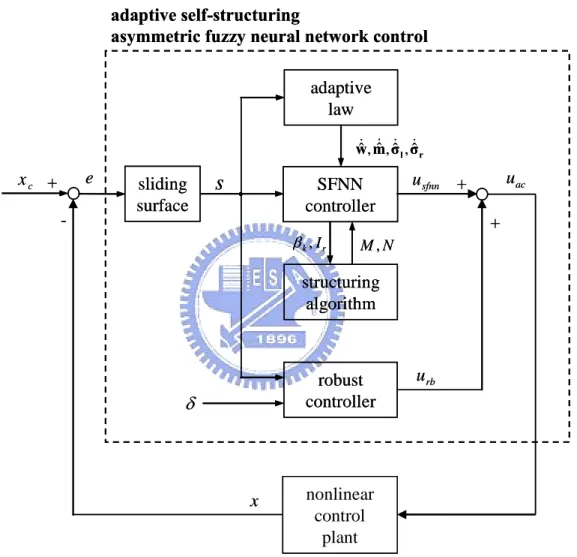
(24) solve the problem of the model-based control approach for real-time implementation, adaptive fuzzy neural-network control (AFNC) techniques have been developed to control these kinds of unknown nonlinear dynamic systems [11-14]. These techniques use a structure of FNN to estimate the plant or controller parameters in a real-time environment. If the FNN is applied to estimate the model of the plant, it is called an indirect AFNC, and if the FNN is applied to estimate the controller of the plant, it is called a direct AFNC [44].. adaptive self-structuring asymmetric fuzzy neural network control adaptive law ˆ& , σˆ& l , σˆ& r ˆ& , m w. e. xc +. -. sliding surface. s. SFNN controller βk , Ir. uac. u sfnn +. + M,N. structuring algorithm. robust controller. δ. u rb. nonlinear control plant. x. Fig. 2-1. The block diagram of ASAFNC system. According to the design concept of the direct AFNC, we propose an adaptive self-structuring asymmetric fuzzy neural-network control (ASAFNC) system as shown in Fig. 2-1. The ASAFNC system is composed of a SFNN controller and a robust controller as u ac = u sfnn + u rb. (2-5). The SFNN controller u sfnn utilizes the SFNN with asymmetric Gaussian membership. 8.

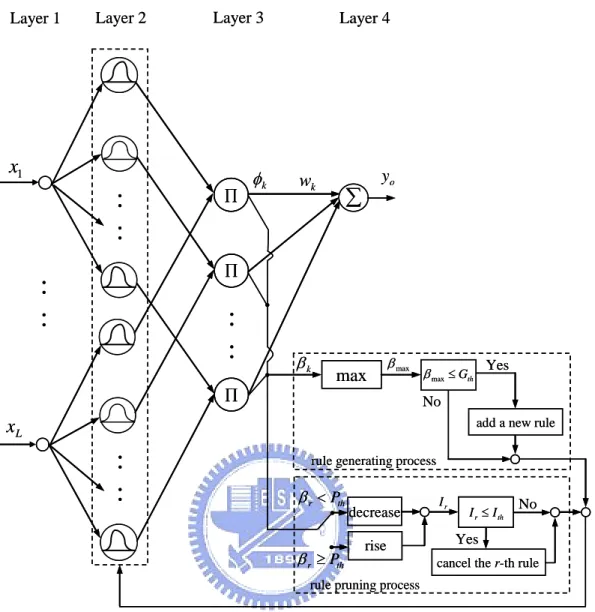
(25) functions to mimic the ideal controller in (2-3), and the robust controller u rb is designed to compensate for the modeling error between the SFNN controller u sfnn and the ideal controller u * . For further analysis, first define a sliding surface as t. s = e ( n −1) + k n e ( n − 2) + L + k 2 e + k1 ∫ e dτ .. (2-6). 0. Substituting (2-5) into (2-1) and using (2-3) and (2-6), yields s& = u * − u sfnn − u rb .. (2-7). 2.2 Description of SFNN. Fuzzy logic and NNs are complementary technologies in the design of intelligent systems. FNNs retain the basic properties and functions of NNs with some of their elements being fuzzified. In this approach, a network’s domain knowledge becomes formalized in terms of fuzzy sets, later being applied to enhance the learning of the network and augment its interpretation capabilities. By incorporating fuzzy principles into a NN, more user flexibility is attained and the resultant network or system becomes more robust [4]. FNNs are generally a fuzzy inference system constructed from structure of NN. Learning algorithms are used to adjust the weightings of the fuzzy inference system. Figure 2-2 shows the configuration of the proposed SFNN which is composed of the input, the membership, the rule, and the output layers. Layer 1 accepts the input variables. Nodes at layer 2 are term nodes which act as membership functions to represent the terms of the respective linguistic variables. The asymmetric Gaussian membership function constituted by a center, a left-side variance, and a right-side variance is considered. Nodes of layer 3 are regarded as fuzzy rules. The links before layer 3 represent the preconditions of rules and the links after layer 3 represent the consequences. Layer 4 is the output layer, where the node in this layer is the output of the NN. The interactions for those layers are given as follows.. 9.

(26) Layer 1. Layer 3. Layer 2. x1 ∏. ：：. Layer 4. φk. wk. yo. ∑. ∏. ：：. ：：. βk. max. ∏. β max. Yes. β max ≤ Gth. No add a new rule. xL. ：：. rule generating process. β r < Pth β r ≥ Pth. decrease rise. Ir. I r ≤ I th. No. Yes cancel the r-th rule. rule pruning process. Fig. 2-2. The structure of SFNN.. Layer 1 - Input layer: For every node i in this layer, the net input and the net output are. represented as 1. (. net i = 1xi. ). yi = 1f i 1 neti = 1neti , i = 1, 2,L, L. 1. (2-8) (2-9). where 1 xi represents the ith input to the node of layer 1 and L is the total number of input variables. They mean that output equals input in this layer. This layer of SFNN just executes the transmission work. Layer 2 - Membership layer: In this layer, each node performs a membership function and. acts as a unit of memory. The bell-shaped function is adopted as the membership function. For the ith input, the corresponding net input and output of the jth node can be expressed as. 10.

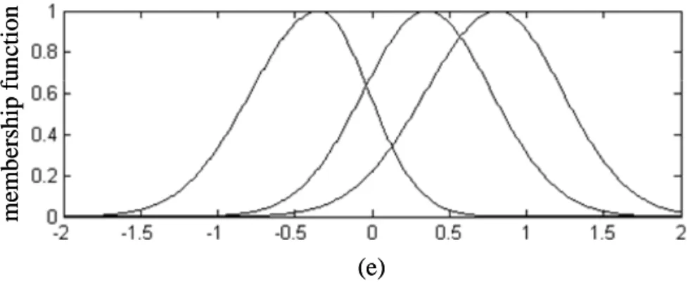
(27) 2. netij. ( =−. 2. xi − 2 mij. (σ ) ) = exp( net ),. ). 2. (2-10). 2. 2. ij. 2. where. 2. (. yij = 2f ij 2 net ij. 2. ij. j = 1, 2,L, M. (2-11). mij is the mean, 2σ ij is the variance and M is the total number of membership. functions with respect to the respective input node. In this study, the input linguistic variable is the tracking error vector. Layer 3 - Rule layer: Each node k in this layer is denoted by ∏ which multiplies the. incoming signals and outputs the result of the product. For the kth rule node, the operation of the net input and output of this layer is presented as net k = ∏ 3 wij 3xij. (2-12). yk = 3f k ( 3 net k ) = 3net k , k = 1, 2,L, N. (2-13). 3. 3. where. 3. xij represents the i, j th input to the kth node of layer 3,. 3. wij between the. membership and the rule layers are assumed as unity, and N is the total number of fuzzy rules. Layer 4 - Output layer: The single node o in this layer is labeled as Σ , which computes the. overall output as the summation of all incoming signals. It executes the sun-of-weighting defuzzification. The description of the net input and output is expressed as net o = ∑ 4 wk 4 x k. (2-14). yo = 4f o ( 4 net o ) = 4 net o. (2-15). 4. k. 4. where. 4. wk is the output action strength of the output associated with the kth rule,. represents the kth input to the node of layer 4, and. 4. 4. xk. yo is the output of SFNN.. In order to improve the learning capability and flexibility of a NN, asymmetric Gaussian membership functions are adopted, instead of ball-shaped functions described in layer 2. According to the above description, the output of the SFNN with N existing fuzzy rules can be represented simply as N. y o = ∑ wk φ k (x). (2-16). k =1. in which wk is the output action strength associated with the k-th rule and φ k is the response of the firing weight for an input vector x = [ x1 x 2 L x L ]T and composed of asymmetric Gaussian membership functions defined as [42]. 11.

(28) (. ⎧ x − mij ⎪exp(− i 2 ⎪⎪ σ ijl ζ ij = ⎨ xi − mij ⎪ ⎪exp(− 2 σ ijr ⎪⎩. (. ( ). ( ). ). 2. ). ), if − ∞ < xi ≤ mij. , j = 1, 2,L, M. 2. (2-17). ), if mij ≤ xi < ∞. where M is the total number of membership functions with respect to the respective input node; mij , σ ijl , and σ ijr are the mean, left-side variance, and right-side variance of the asymmetric Gaussian function in the j-th term of the i-th input linguistic variable xi , respectively. However, σ ijl and σ ijr may become zero in the training procedure, the membership function ζ ij will not be defined. To avoid this problem, this dissertation considers a membership function form as [44] ⎧ ⎪exp(− ⎪⎪ ζ ij = ⎨ ⎪ ⎪exp(− ⎪⎩. (x − m ) ), if (σ ) + ϖ (x − m ) ), if (σ ) + ϖ 2. i. − ∞ < xi ≤ mij. ij. l 2 ij. , j = 1, 2,L, M. 2. i. (2-18). mij ≤ xi < ∞. ij. r 2 ij. where ϖ is a small positive constant. Then, the associated firing strength can be defined as M. φ k = ∏ ζ jk .. (2-19). j =1. To note easily, define vectors m , σ l , and σ r collecting all parameters of SFNN as m = [m11 L m L1 m12 L m L 2 LL m1M L m LM ]T. (2-20). l σ l = [σ 11l L σ Ll 1 σ 12l L σ Ll 2 LL σ 1lM L σ LM ]T. (2-21). r σ r = [σ 11r L σ Lr1 σ 12r L σ Lr 2 LL σ 1rM L σ LM ]T .. (2-22). Thus, the output of the SFNN can be represented in a vector form as y o = w T φ(x, m, σ l , σ r ). (2-23). where w = [ w1 w2 L wN ]T and φ = [φ1 φ 2 L φ N ]T . For the FNN approaches, the structure of the FNN should be determined in advance by empiricism. However, it is difficult to consider the balance between the rule number and the desired performance. Therefore, the structure adaptation algorithm which contains the growing and pruning of membership functions and fuzzy rules is proposed in this dissertation. The descriptions are given as follows. In the process of the growing of membership functions, the concept which decides. 12.

(29) whether to add a new node (membership function) in layer 2 and the associated fuzzy rule in layer 3 will be introduced. The mathematical description of the existing rules can be expressed as a set of clusters. For constructing the initial fuzzy rules of the SFNN, the fuzzy clustering method is used to partition a set of data into a number of overlapping clusters based on the distance in a metric space between the data points and the cluster prototypes. Each cluster in the product space of the input-output data represents a rule. The firing strength of a rule for each incoming data xi can be represented as the degree that the incoming data belong to the cluster [19]. If the value of firing strength is too small, it indicates that the input value is on the edge of range of the existing membership functions. Under this situation, the output will cause unsatisfactory performance. Therefore, a new membership function and a new fuzzy rule should be generated to improve the performance. The firing strength from (2-19) is used as the degree measure. β k = φ k , k = 1, 2, ..., N (t ). (2-24). where N (t ) is the number of the existing fuzzy rules at the time t. Define the maximum degree β max as. β max = max β k . 1≤ k ≤ N ( t ). (2-25). If β max ≤ Gth is satisfied, where Gth ∈ (0,1) is a pre-given threshold, the incoming data is far from the edge of range of the existing membership functions. Hence, a new membership function is generated. The mean and the variance of the new membership function and the weight are selected as follows minew = xi ,. (2-26). σ il , new = σ i ,. (2-27). σ ir , new = σ i ,. (2-28). w new = 0. (2-29). where xi is the new incoming data and σ i is a pre-specified constant. If the unknown control system dynamics is too complex, we can choose the larger Gth so that many membership functions can be created.. 13.

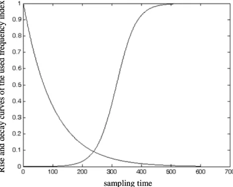
(30) Rise and decay curves of the used frequency index. sampling time. Fig. 2-3. The rise and decay curves of the used frequency index.. Next, to avoid the unrestricted growth of network structure and an overload computation, the pruning algorithm is developed to eliminate irrelevant fuzzy rules. In Ref. [21], a significance index is determined for the importance of the fuzzy rules. The elimination algorithm is derived from the observation that if the significance index fades when the firing weight is smaller than a special threshold value and if the significance index fixes when the firing weight is larger than a special threshold value [21]. In this dissertation, when the r-th firing strength β r is smaller than the threshold value Pth , it indicates that the relationship becomes weak between the input and the r-th rule. Then, the significant index of r-th fuzzy rules will be decreased. When the r-th firing strength β r is larger than the threshold value Pth , it indicates that the incoming inputs fall into the range of the r-th fuzzy rule. Thus, the significant index of r-th fuzzy rules should be raised. The rise and decay curves of the used frequency index show in Fig. 2-3. The significance index is determined for the r-th rules can be given as ⎧⎪ I r (t ) ⋅ exp(−τ 1 ), if β r < Pth I r (t + 1) = ⎨ , r = 1, 2, L , N (t ) ⎪⎩ I r (t ) ⋅ 2 − exp − τ 2 1 − I r (t ) , if β r ≥ Pth. [. (. ))]. (. (2-30). where I r is the significant index of the r-th rule and its initial value is 1, Pth is the pruning. 14.

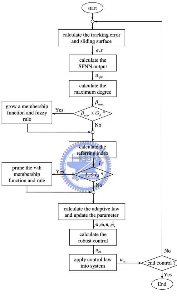
(31) threshold value, and τ 1 and τ 2 are the designed constant. Exponential functions in (2-30) are used to rise or decrease the values of significant index in [0, 1]. If I r ≤ I th is satisfied, where I th is another pre-given threshold, the r-th fuzzy rule will be deleted. For real-time implementation, if the computation load is the issue having highest priority, Pth should be chosen large, so that more fuzzy rules can be pruned. This operation will prevent the fuzzy rule, which may be less used but still significant, from being deleted in the training process. Hence, the computation load would be reduced. In summary, the flow chart of the structure learning algorithm is shown in Fig. 2-4. The major contributions of the SFNN are: 1) SFNN can be operated directly without spending much time pre-determining membership functions and fuzzy rules; and 2) the computation load can be reduced simultaneously.. 15.

(32) start. calculate the tracking error and sliding surface. ee,, s calculate the SFNN output. u sfnn calculate the maximum degree grow a membership function and fuzzy rule. β max Yes. β max ≤ Gth ? No. calculate the referring index prune the r-th membership function and rule. Ir Yes. I r ≤ I th ? No. calculate the adaptive law and update the parameter &ˆ , m ˆ& , σˆ& l , σ&ˆ r w. calculate the robust control. urb apply control law into system. No. uac. end control ? Yes End. Fig. 2-4. The flow chart of the ASAFNC system.. 16.

(33) 2.3 Approximation of SFNN. An optimal SFNN controller can be designed to approximate the ideal controller (2-3) even under the structural change of neural network, such that [44, 45] * u * = u sfnn + ∆ = w *T φ ( x, m * , σ *l , σ *r ) + ∆ = w *T φ * + ∆. (2-31). where φ * = φ(x, m * , σ *l , σ *r ) , ∆ denotes the approximation error, and w * , m * , σ *l , and. σ *r are the optimal vectors. In fact, the optimal vectors that best approximate a given nonlinear function are difficult to be determined. Thus, an estimated SFNN controller is introduced as ˆ , σˆ l , σˆ r ) = w ˆ T φ ( x, m ˆ T φˆ u sfnn = w. (2-32). where φˆ = φ(x, m ˆ , σˆ l , and σˆ r are the estimated vectors of w , m , ˆ , σˆ l , σˆ r ) and w ˆ, m. σ l , and σ r , respectively. Moreover, the optimal vectors can be further defined as [44] (w * , m * , σ *l , σ *r ) =. arg min. ˆ ∈Ω m , σˆ l ∈Ω σ l ,σˆ r ∈Ω σ r ˆ ∈Ω w , m w. ⎡ ⎤ * ˆ , σˆ l , σˆ r ) ⎥ u sfnn (x) − u sfnn (x, m ⎢ x∈sup ⎣ Ωx ×R ⎦. (2-33). where ˆ: w ˆ ≤ Dw } Ωw = { w. (2-34). ˆ:m ˆ ≤ Dm } Ωm = { m. (2-35). { = { σˆ. } ≤D }. Ω σ l = σˆ l : σˆ l ≤ Dσ l. (2-36). Ω σr. (2-37). r. : σˆ r. σr. where Dw , Dm , Dσ l , and Dσ r are positive constants specified by designers. There exists. ∆* which is a finite positive constant such that the inequality ∆ ≤ ∆* can be held. Define a modeling error, u~ , as. ~+w ~+w ~ Tφ ~ T φˆ + ∆ ˆ Tφ u~ = u * − u sfnn = w. (2-38). ~ = φ * − φˆ . In the following description, the linearization ~ = w* − w ˆ and φ where w technique is employed to transform the nonlinear fuzzy function into a partially linear form so ~ can be expressed as [46] that the expansion φ. 17.

(34) ⎡ ∂φ1 ⎡ ∂φ1 ⎤ ⎢ ∂σ ⎡ φ1 ⎤ ⎢ ∂m ⎥ ⎢ l ⎢ ~ ⎥ ⎢ ∂φ 2 ⎥ ⎢ ∂φ 2 φ2 ⎥ ⎢ ⎥ * ~ ⎢ ˆ ) + ⎢ ∂σ φ= (m − m = l ⎢ M ⎥ ⎢ ∂m ⎥ ⎢ M ⎥ ⎢ M ⎢~ ⎥ ⎢ ∂φ ⎢⎣φ N ⎥⎦ ⎢ ∂φ N ⎥ ⎢ N ⎢⎣ ∂m ⎥⎦ ˆ m =m ⎣⎢ ∂σ l ~. ⎡ ∂φ1 ⎤ ⎢ ∂σ ⎥ ⎢ r ⎥ ⎢ ∂φ 2 ⎥ * (σ l − σˆ l ) + ⎢ ∂σ ⎥ r ⎢ M ⎥ ⎢ ∂φ ⎥ ⎢ N ⎥ ⎣⎢ ∂σ r ⎦⎥ σ =σˆ l. l. ⎤ ⎥ ⎥ ⎥ ⎥ ⎥ ⎥ ⎥ ⎦⎥ σ. (σ *r − σˆ r ) + h. ˆr r =σ. T ~ ~ + φT σ ~ = φ Tm m σl l + φ σr σ r + h. (2-39). ~ = m* − m ~ = σ* − σˆ , and σ ~ = σ* − σˆ . ˆ , σ where h is a vector of higher-order term, m l l l r r r Substituting (2-39) into (2-38), (2-38) can be rewritten as ~+w ~ + φT σ ~ Tφ ~ + φT σ ~ + h) + w ~ T φˆ + ∆ ˆ T (φT m u~ = w m. σl. l. σr. r. ~ Tφ w ~ T φˆ + m ~T φ w ~T φ w ˆ +σ ˆ +σ ˆ +ε =w m l r σl σr. (2-40). ~ Tφ w ~, σ ~T φ w ~, σ ~T φ w ~ , and the uncertain term ˆ =w ˆ T φTmm ˆ =w ˆ T φTσ l σ ˆ T φTσ r σ where m m l σl l r σr ˆ = w r ~ + ∆ . The higher-order term h satisfies ~ Tφ ε = wˆ T h + w T ~ ~ − φT m ~ − φT σ ~ h = φ m σl l − φ σr σ r. ~ + φT m ~ + φT σ ~ + φT σ ~ ≤ φ m σl l σr r ~ +c σ ~ +c σ ~ ≤ c 0 + c1 m 2 l 3 r. (2-41). ~ ≤ c , φT ≤ c , φT ≤ c , where c 0 , c1 , c 2 , and c 3 are positive constants satisfying φ 1 2 0 m σl. φTσ r ≤ c 3 . The existence of c 0 , c1 , c 2 , and c 3 is assured due to the fact that Gaussian ~, σ ~, m ~ , and σ ~ function and its derivative are always bounded by constants. Moreover, w l r satisfy. ~ = w* − w ˆ ≤ w* + w ˆ ≤ Dw + w ˆ w. (2-42). ~ = m* − m ˆ ≤ m* + m ˆ ≤ Dm + m ˆ m. (2-43). ~ = σ * − σˆ ≤ σ * + σˆ ≤ D + σˆ σ l l l l l σl l. (2-44). ~ = σ * − σˆ ≤ σ * + σˆ ≤ D + σˆ . σ r r r r r σr r. (2-45). Next, the uncertain term ε is satisfied ~ + φT σ ~ T (φT m ~ + φT σ ~ + h) + w ˆ Th + ∆ ε = w m σ l σ r l. r. *T ~ +w ~ T φT m ~ T φT σ ~ ~T T ~ = w m σ l l + w φσ r σr + w h + ∆. 18.

(35) ˆ ) + c 2 ( Dw + w ˆ )( Dm + m ˆ )( Dσ l + σˆ l ) + c 3 ( Dw + w ˆ )( Dσr + σˆ r ) ≤ c1 ( Dw + w ˆ ) + c 2 ( Dσ l + σˆ l ) + c 3 ( Dσr + σˆ r )] + ∆* + Dw [c 0 + c1 ( Dm + m ˆ , σˆ l , σˆ r , m ˆ w ˆ ,m ˆ , σˆ l w ˆ , σˆ r w ˆ ]T = [Θ1 , Θ 2 , Θ 3 , Θ 4 , Θ 5 , Θ 6 , Θ 7 , Θ 8 ][1, w. = ΘT Γ. (2-46). where Θ = [Θ1 , Θ 2 , Θ 3 , Θ 4 , Θ 5 , Θ 6 , Θ 7 , Θ 8 ]T , Θ1 = (c 0 + 2c1 Dm + 2c 2 Dσ + 2c 3 Dσ ) Dw + ∆* , l r Θ 2 = c1 Dm + c 2 Dσ l + c 3 Dσ r , Θ 3 = 2c1 Dw , Θ 4 = 2c 2 Dw , Θ 5 = 2c 3 Dw , Θ 6 = c1 , Θ 7 = c 2 , ˆ , σˆ l , σˆ r , m ˆ w ˆ ,m ˆ , σˆ l w ˆ , σˆ r w ˆ ]T . Since Θ is a bounded vector, Θ 8 = c 3 and Γ = [1, w. if Γ can be guaranteed to be bounded, the uncertain term ε is bounded. The analysis of boundness of Γ will be given in the later section.. 2.4 ASAFNC Design. By using (2-40), (2-7) can be rewritten as ~ Tφ w ~ T φˆ + m ~T φ w ~T φ w ˆ +σ ˆ +σ ˆ + ε − u rb . s& = w m l σl r σr. (2-47). If ε exists, consider a specified L2 tracking performance [46, 47]. ∫. T 0. T. s 2 (t )dt ≤ s 2 (0) + δ 2 ∫ ε 2 (t )dt + 0. 1 ~T ~ 1 ~T ~ (0) w (0)w (0) + m (0)m. ηw. 1 ~T ~ 1 ~T ~ + σ l (0)σ l (0) + σ r (0)σ r (0). ησ. ησ. l. ηm. (2-48). r. where η w , η m , ησ l , and ησ r are the positive-constant learning rates, and δ is a prescribed attenuation constant. If the system starts with initial conditions s (0) = 0 , ~ (0) = 0 , σ ~ (0) = 0 , m ~ (0) = 0 , and σ ~ (0) = 0 , the L tracking performance in (2-48) can w l r 2 be rewritten as sup. ε ∈L2 [ 0 ,T ]. where. s. 2. T. = ∫ s 2 (t )dt and 0. ε. 2. s. ε. ≤δ. (2-49). T. = ∫ ε 2 (t )dt . If δ = ∞ , this is the case of minimum 0. error tracking control without disturbance attenuation. To determine the adaptive laws of the parameters of ASAFNC appropriately and guarantee the closed-loop system stability, the Lyapunov function candidate is defined as. 19.

(36) V =. ~T σ ~ σ ~T σ ~ ~ Tm ~ σ ~Tw ~ m 1 2 w s + + + l l + r r. 2 2η w 2η m 2ησ l 2η σ r. (2-50). Differentiating (2-50) with respect to time and using (2-47) yield ~ Tm ~& σ ~Tw ~& m ~T σ ~& ~T σ ~& w σ V& = ss& + + + l l+ r r. ηw. ηm. ησ. ησ. l. r. ~ Tm ~& σ ~T σ ~& ~T σ ~& ~Tw ~& m σ w ~ Tφ w ~ T φˆ + m ~T φ w ~T φ w l l r r ˆ ˆ ˆ = s(w + + + − + + + + σ σ u ) ε rb m l σl r σr. ηw. ηm. ησ. l. ησ. r. 1 ~& ~ T 1 ~& ~ T ( sφ w ~ T ( sφˆ + 1 w ~& ) + m ˆ+ ˆ+ =w m ) + σ l ( sφ σ l w σl ) m. ηw. ηm. ησ. l. 1 ~& ~ T ( sφ w ˆ+ +σ σ r ) + s (ε − u rb ) r σr. ησ. (2-51). r. Choose the adaptive laws as ~& = − w ˆ& = −η w sφˆ w. (2-52). ~& = −m ˆ& = −η m sφ m w ˆ m. (2-53). ~& = −σ&ˆ = −η sφ w ˆ σ l l σl σl. (2-54). ~& = −σˆ& = −η sφ w ˆ σ r r σr σr. (2-55). and the robust controller is designed as u rb =. δ 2 +1 s. 2δ 2. (2-56). Thus, equation (2-51) can be rewritten as. δ 2 +1 V& = s (ε − s) 2δ 2 = sε − =−. s2 s2 − 2 2 2δ. s2 1 s 1 − ( − εδ ) 2 + ε 2δ 2 2 2 δ 2. 1 1 ≤ − s 2 + ε 2δ 2 . 2 2. (2-57). Assume ε ∈ L2 [0, T ] , ∀T ∈ [0, ∞) . Integrating the above equation from t = 0 to t = T yields V (T ) − V (0) ≤ −. T 1 T 2 1 s dt + δ 2 ∫ ε 2 dt . ∫ 0 2 0 2. 20. (2-58).

(37) Since V (t ) ≥ 0 , we can arrange (2-58) as follows 1 T 2 1 2 T 2 ( 0 ) s dt ≤ V + δ ε dt 2 ∫0 2 ∫0. (2-59). which is equivalent to inequality (2-48) , i.e., L2 tracking performance. Assume ε ∈ L2 , then the sliding surface s will converge to a certain small boundary. It is implied that the tracking error e will also converge to a certain small boundary [47].. 2.5 Boundary Analysis Using Projection Algorithm ˆ , σˆ l , and ˆ, m Although the stability of ASAFNC can be guaranteed, the parameters w. σˆ r cannot be guaranteed within a desired bound value by using the adaptive laws (2-52)-(2-55). According to the projection algorithm [44, 48, 49], the adaptive laws can be modified as follows. The adaptive law of weight is ⎧ η sφˆ , ˆ < Dw or ( w ˆ = Dw and sw ˆ T φˆ ≤ 0) if w ˆ& = ⎨ w w ˆ = Dw and sw ˆ T φˆ > 0) ⎩Pr (η w sφˆ ) , if ( w. (2-60). where the projection operator is given as Pr (η w sφˆ ) = η w sφˆ − η w s. ˆ T φˆ w ˆ w. 2. ˆ . w. (2-61). The adaptive law of mean of asymmetric membership function is ˆ < Dm or ( m ˆ = Dm and sm ˆ T φm w ⎧ η m sφ m w ˆ , ˆ ≤ 0) if m & ˆ m=⎨ ˆ = Dm and sm ˆ T φm w ˆ ) , if ( m ˆ > 0) ⎩Pr (η m sφ m w. (2-62). where the projection operator is given as ˆ ) = η m sφ m w ˆ −ηm s Pr (η m sφ m w. ˆ T φm w ˆ m ˆ m. 2. ˆ . m. (2-63). The adaptive law of left-side variance of asymmetric membership function is. ⎧⎪ησ sφ σ l w ˆ , ˆ ≤ 0) if σˆ l < Dσ l or ( σˆ l = Dσ l and sσˆ Tl φ σ l w σˆ& l = ⎨ l T ˆ ) , if ( σˆ l = Dσ l and sσˆ l φ σ l w ˆ > 0) ⎪⎩Pr (ησ l sφ σ l w. (2-64). where the projection operator is given as ˆ ) = η σ l sφ σ l w ˆ − ησ l s Pr (ησ l sφ σ l w. T ˆ σˆ l φ σ l w. σˆ l. 2. σˆ l .. The adaptive law of right-side variance of asymmetric membership function is 21. (2-65).

(38) ˆ, ˆ ≤ 0) if σˆ r < Dσr or ( σˆ r = Dσ r and sσˆ Tr φ σr w &σˆ = ⎧⎪ησ r sφ σr w ⎨ r T ˆ ) , if ( σˆ r = Dσ r and sσˆ r φ σr w ˆ > 0) ⎪⎩Pr (ησ r sφ σr w. (2-66). where the projection operator is given as. ˆ ) = ησ r sφ σ r w ˆ − ησ r s Pr (ησ r sφ σ r w. ˆ σˆ Tr φ σ r w σˆ r. 2. σˆ r .. (2-67). ˆ (0) ∈ Ω m , σˆ l (0) ∈ Ω σ l , and σˆ r (0) ∈ Ω σ r , ˆ (0) ∈ Ω w , m Then, let the initial values satisfy w ˆ (t ) ∈ Ω m , σˆ l (t ) ∈ Ω σ l , and σˆ r (t ) ∈ Ω σ r can be kept for all ˆ (t ) ∈ Ω w , m the conditions w ˆ , σˆ l , and σˆ r ˆ , m t ≥ 0 , i.e., w. are all bounded.. Thus, the fact that the uncertain term ε is bounded can be guaranteed by the modified adaptive laws (2-60), (2-62), (2-64), and (2-66). The following description states that the analytic result of stability is the same as (2-59) by re-selecting the adaptive laws (2-60), (2-62), (2-64), and (2-66). First, define some useful variables as. ~& ) ~ T ( sφˆ + 1 w Jw = w. (2-68). 1 ~& ~ T ( sφ w ˆ + m) Jm = m m. (2-69). 1 ~& σl ). (2-70). ηw. ηm. ~ T ( sφ w ˆ + J σl = σ l σl. ησ. l. and ~ T ( sφ w ˆ + J σr = σ r σr. 1 ~& σr ) .. ησ. (2-71). r. Then, the derivative of Lyapunov function shown in (2-51) can be rewritten as V& = J w + J m + J σ l + J σ r + s (ε − u rc ) .. (2-72). By using (2-60), J w = 0 for [ w ˆ < Dw or ( w ˆ = Dw and sw ˆ T φˆ ≤ 0) ] can be obtained. For ( w ˆ = Dw and sw ˆ T φˆ > 0) , Jw = s. ~Tw ˆ w ˆ w. 2. ˆ T φˆ . w. (2-73). can be obtained. Because w * belongs to the constraint set Ω w , we have w ˆ = Dw ≥ w * .. 1 ~Tw Using this fact, we obtain w ˆ = ( w* 2. 2. 2 ~ 2 ) ≤ 0 . Thus, equation (2-73) can be ˆ − w − w. rewritten as. 22.

(39) s(w Jw = 2. * 2. 2 ~ 2) ˆ − w − w. ˆ w. 2. ˆ T φˆ ≤ 0 . w. (2-74). Similarly, by using (2-62), J m = 0 can be obtained for [ m ˆ < Dm or ( m ˆ = Dm. and. ˆ T φm w ˆ = Dm and sm ˆ T φm w ˆ ≤ 0) ] ; and for ( m ˆ > 0) , the inequality sm s (m Jm = 2. * 2. 2 ~ 2) ˆ − m − m. ˆ m. 2. ˆ T φm w ˆ ≤0 m. (2-75). can be obtained. By using (2-64), we obtain J σ = 0 for [ σˆ l < Dσ or ( σˆ l = Dσ and l l l ˆ ≤ 0) ] ; and for ( σˆ l = Dσ l and sσˆ Tl φ σ l w ˆ > 0) , the inequality sσˆ Tl φ σ l w * 2. J σl. s ( σl = 2. − σˆ l. 2. σˆ l. 2. ~ 2) − σ l. J σr = 0. can be obtained. By using (2-66),. T ˆ ≤0 σˆ l φ σ l w. for [ σˆ r < Dσ r. (2-76) or. ( σˆ r = Dσ r. and. ˆ ≤ 0) ] ; and for ( σˆ r = Dσ r and sσˆ Tr φ σ r w ˆ > 0) , the inequality sσˆ Tr φ σr w * 2. J σr. s ( σr = 2. − σˆ r. 2. σˆ r. 2. ~ 2) − σ r. ˆ ≤0 σˆ Tr φ σ r w. (2-77). can be obtained. Hence, for any possible condition occurs in (2-60), (2-62), (2-64), and (2-66), the conditions J w ≤ 0 , J m ≤ 0 , J σ ≤ 0 , and J σ ≤ 0 can be satisfied. Then, (2-72) can be l r reorganized as V& = J w + J m + J σ l + J σ r + s (ε − u rb ). ≤ s(ε − u rb ) .. (2-78). By substituting the robust controller (2-56), (2-78) can be rewritten as. δ 2 +1 & V ≤ s (ε − s) 2δ 2 1 s2 1 s = − − ( − εδ ) 2 + ε 2δ 2 2 2 δ 2 1 1 ≤ − s 2 + ε 2δ 2 . 2 2. (2-79). Using the same discussion in the section 2.4, the stability of the system with the projection algorithm can also be guaranteed.. 23.

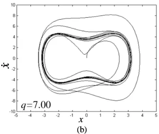
(40) 2.6 Simulation Results. In this section, the proposed ASAFNC is applied to a second-order chaotic dynamics system to verify its effectiveness. This scheme emphasizes that the parameter and network structure of the SFNN can be tuned online by the proposed algorithm. Consider a second-order chaotic dynamics system such as the Duffing’s equation describing a special nonlinear circuit or a pendulum moving in a viscous medium as follows [46] &x& = f (x) + u. (2-80). where f (x) = − px& − p1 x − p 2 x 3 + q cos(ωt ) is the system dynamics, t is the time variable,. ω is the frequency, u is the control force, and p , p1 , p 2 , and q are real constants. The solutions of (2-80) may exhibit periodic depending on the choice of these constants, i.e., it is almost periodic and chaotic behavior. The open-loop system behavior, i.e., u = 0 , is simulated with p = 0.4 , p1 = −1.1 , p 2 = 1.0 , and ω = 1.8 for observing the chaotic unpredictable behavior. The phase plane plots with an initial condition point (0, 0) are shown in Figs. 2-5(a) and 2-5(b) for q = 1.95 and q = 7.00 , respectively. The uncontrolled chaotic system has different trajectories for different values of q. To illustrate the effectiveness of the proposed design method, a comparison among a fix-structure AFNC using symmetric Gaussian membership functions [50], a fix-structure AFNC using asymmetric Gaussian. x&. membership functions [51], and the proposed ASAFNC is made.. q=1.95. x (a). 24.

(41) x& q=7.00 x (b). Fig. 2-5. Phase plane of uncontrolled chaotic dynamics system.. 2.6.1 Comparison with AFNC. The simulation results of fix-structure AFNC using 3 symmetric membership functions are shown in Fig. 2-6. The tracking responses of state x are shown in Figs. 2-6(a) and 2-6(d); the tracking responses of state x& are shown in Figs. 2-6(b) and 2-6(e); and the associated control efforts are shown Figs. 2-6(c) and 2-6(f) for q = 1.95 and q = 7.00 , respectively. The simulation results show that the tracking responses decline when membership functions are selected insufficiently.. state, x. xc. x. time (sec) (a). 25.

(42) state, x&. x&c. x&. control effort. time (sec) (b). time (sec) (c). state, x. xc. x. time (sec) (d). state, x&. x&c. x& time (sec) (e). 26.

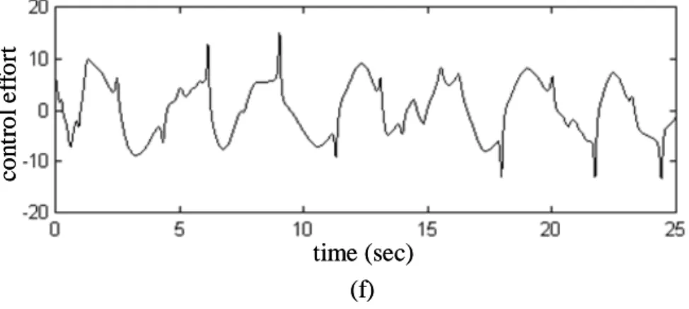
(43) control effort. time (sec) (f). Fig. 2-6. Simulation results of AFNC using 3 symmetric membership functions.. Next, the simulation results of fix-structure AFNC using 20 symmetric membership functions are shown in Fig. 2-7. The tracking responses of state x are shown in Figs. 2-7(a) and 2-7(d); the tracking responses of state x& are shown in Figs. 2-7(b) and 2-7(e); and the associated control efforts are shown Figs. 2-7(c) and 2-7(f) for q = 1.95 and q = 7.00 , respectively. The simulation results show that the favorable tracking performance can achieve; however, the computation load is heavy. These results demonstrate the fact that it is difficult to consider the balance between the rule number and the desired performance.. state, x. xc. x. time (sec) (a). 27.

(44) state, x&. x&. x&c. control effort. time (sec) (b). time (sec) (c). state, x. xc. x. time (sec) (d). state, x&. x&. x&c. time (sec) (e). 28.

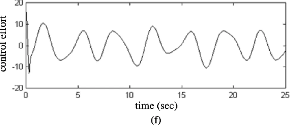
(45) control effort. time (sec) (f). Fig. 2-7. Simulation results of AFNC using 20 symmetric membership functions.. To show that the learning capability of neural network can be upgraded as using the asymmetric Gaussian membership functions, the fix-structure AFNC using asymmetric Gaussian membership functions is applied to chaotic dynamics system again. The simulation results of fix-structure AFNC using 3 asymmetric membership functions are shown in Fig. 2-8. The tracking responses of state x are shown in Figs. 2-8(a) and 2-8(d); the tracking responses of state x& are shown in Figs. 2-8(b) and 2-8(e); and the associated control efforts are shown Figs. 2-8(c) and 2-8(f) for q = 1.95 and q = 7.00 , respectively. The simulation results show that the favorable tracking performance can be achieved.. state, x. xc. x. time (sec) (a). 29.

(46) state, x&. x&c. x&. control effort. time (sec) (b). time (sec) (c). state, x. x. xc. time (sec) (d). state, x&. x&c. x& time (sec) (e). 30.

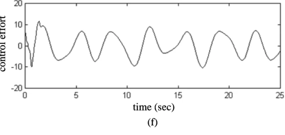
(47) control effort. time (sec) (f). Fig. 2-8. Simulation results of AFNC using 3 asymmetric membership functions.. Next, the simulation results of fix-structure AFNC using 20 asymmetric membership functions are shown in Fig. 2-9. The tracking responses of state x are shown in Figs. 2-9(a) and 2-9(d); the tracking responses of state x& are shown in Figs. 2-9(b) and 2-9(e); and the associated control efforts are shown Figs. 2-9(c) and 2-9(f) for q = 1.95 and q = 7.00 , respectively. The simulation results show that the favorable tracking performance can achieve; however, the computation load is heavy. Comparing with Figs. 2-6 and 2-8, and Figs. 2-7 and 2-9 shows that the adaptive fuzzy neural network with asymmetric membership functions performs better than the adaptive fuzzy neural network with symmetric membership functions. However, the structure of the FNN should still be determined by the empiricism.. state, x. xc. x. time (sec) (a). 31.

(48) state, x&. x&. x&c. control effort. time (sec) (b). time (sec) (c). state, x. xc. x. time (sec) (d). state, x&. x&. x&c. time (sec) (e). 32.