論貨幣政策與資產價格 - 政大學術集成
96
0
0
全文
(2) 立. 政 治 大. ‧. ‧ 國. 學. n. er. io. sit. y. Nat. al. Ch. engchi. i n U. v.
(3) 論貨幣政策與資產價格 Essays on Monetary Policy and Asset Prices. 立. 政 治 大 A Dissertation. ‧ 國. 學. by Philipp Klotz. ‧. Nat. sit. y. Submitted to National Chengchi University. io. n. al. Doctor of Philosophy. Ch. engchi. er. in partial fulfillment of the requirements for the degree of. i n U. v. Chair of Committee. Dr. Tsoyu Calvin Lin 林左裕 博士. Committee Members. Dr. Chung-Rou Fang 方中柔 博士 Dr. Shih-Hsun Hsu 徐士勛 博士 Dr. Che-Chun Lin 林哲群 博士 Dr. Tzu-Chin Lin 林子欽 博士 Dr. Tony Shun-Te Yuo 游舜德 博士. 中華民國一百零三年三月.
(4) 立. 政 治 大. ‧. ‧ 國. 學. n. er. io. sit. y. Nat. al. Ch. engchi. i n U. v.
(5) Abstract This thesis consists of two essays on the relationship between monetary policy and asset price dynamics. The first essay examines the extent to which Greece, Ireland, Portugal and Spain experienced property bubbles and investigates the role of European Central Bank’s (ECB) monetary policy in the formation of these bubbles in the period from 1999 to 2012. The analysis shows that Spain and Ireland experienced the largest bubble formation followed by Portugal and Greece. Cointegration tests and VEC impulse responses indicate a significant long- and short-run relationship. 政 治 大 The second essay examines long- and short-run dynamics between global commodity 立 between ECB’s monetary policy and bubble formation in Greece, Ireland and Spain.. ‧ 國. 學. prices, economic activity and monetary policy of China in the period from 1998M01 to 2012M12. While Toda and Yamamoto (1995) type Granger causality tests provide. ‧. no evidence for a long-run relationship between monetary policy and commodity. sit. y. Nat. prices, VAR generalized impulse responses suggests that agricultural commodity. io. al. er. prices overshoot in response to a drop in the real interest rate. The analysis further. v. n. finds evidence that industrial metals prices tend to be higher when China’s exchange rate regime is relaxed.. Ch. engchi. I. i n U.
(6) Table of Contents 1. Introduction................................................................................................................ 1 2. Monetary Policy and Real Estate Bubbles................................................................. 9 2.1. Introduction .........................................................................................................9 2.2. Literature Review ..............................................................................................16 2.2.1. Real Estate Bubbles ....................................................................................16 2.2.2. Monetary Policy and Property Bubbles ......................................................19 2.3. Framework ........................................................................................................20 2.3.1. Property Bubble Determination..................................................................20 2.3.2. Monetary Policy Transmission ...................................................................23. 政 治 大 2.5. Empirical Analysis ............................................................................................29 立 2.5.1. Long-Run Dynamics ..................................................................................29 2.4. Data ...................................................................................................................25. ‧ 國. 學. 2.5.2. Short-Run Dynamics ..................................................................................32 2.6. Discussion .........................................................................................................37. ‧. 2.7. Conclusion .........................................................................................................41. sit. y. Nat. 3. Monetary Policy and Global Commodity Prices ..................................................... 44 3.1. Introduction .......................................................................................................44. io. n. al. er. 3.2. Framework ........................................................................................................51. i n U. v. 3.3. Data and Methodology ......................................................................................53. Ch. engchi. 3.3.1. Data.............................................................................................................53 3.3.2. Methodology...............................................................................................59 3.4. Empirical Analysis ............................................................................................62 3.4.1. Unit Root Tests and Lag Length Selection.................................................62 3.4.2. VAR Estimation and Model Robustness ....................................................64 3.4.3. Long-Run Dynamics ..................................................................................65 3.4.4. Short-Run Dynamics ..................................................................................67 3.5. Conclusion .........................................................................................................70 4. Conclusion ............................................................................................................... 73 5. References................................................................................................................ 78. II.
(7) List of Abbreviations BGS. British Geological Survey. BIS. Bank for International Settlements. BP. British Petroleum. CBOT. Chicago Board of Trade. CME. Chicago Mercantile Exchange. COMEX. Commodity Exchange. DCE. Dalian Commodity Exchange. EA. 政 治 大 European Central Bank 立. ECB. Euro Area. EMF. European Mortgage Federation. Euribor. Euro Interbank Offered Rate. FAO. Food and Agriculture Organization of the United Nations. GIRF. Generalized Impulse Response Function. GVA. Gross Value Added. er. io. sit. y. Nat. al. v i n C h AutocorrelationUConsistent Heteroskedasticity and engchi n. HAC. ‧. ‧ 國. Energy Information Administration. 學. EIA. ICE. Intercontinental Exchange. KCBOT. Kansas City Board of Trade. LME. London Metal Exchange. LTV. Loan-to-Value. NYBOT. New York Board of Trade. NYMEX. New York Mercantile Exchange. OECD. Organization for Economic Co-operation and Development. OTC. Over-the-Counter III.
(8) PBC. People’s Bank of China. RMB. Renminbi. S.D.. Standard Deviation. SFE. Shanghai Futures Exchange. T&Y. Toda and Yamamoto. USD. US Dollar. USITC. United States International Trade Commission. VAR. Vector Auto Regression. VEC. Vector Error Correction. WACC. 治 政 大 Weighted Average Cost of Capital 立. World Federation of Exchanges. WTO. World Trade Organization. Y-o-Y. Year-on-Year. ZCE. Zhengzhou Commodity Exchange. ‧. ‧ 國. 學. WFE. n. er. io. sit. y. Nat. al. Ch. engchi. IV. i n U. v.
(9) List of Figures Figure 2.1: Residential Property Bubbles with LTV Ratio of 70% ............................. 26 Figure 2.2: Residential Property Bubble Simulation under Varying LTV Ratios ....... 27 Figure 2.3: 3-Month Euribor and Key Policy Rate of the ECB ................................... 28 Figure 2.4: Lending for House Purchase-to-Quarterly GDP in the Eurozone ............. 28 Figure 2.5: Portugal’s Bubble Response to Cholesky One S.D. Innovations .............. 34 Figure 2.6: Greece’s Bubble Response to Cholesky One S.D. Innovations ................ 34 Figure 2.7: Ireland’s Bubble Response to Cholesky One S.D. Innovations ................ 35. 政 治 大 Figure 3.1: Commodity Group Spot Price Indices....................................................... 55 立 Figure 2.8: Spain’s Bubble Response to Cholesky One S.D. Innovations .................. 36. ‧ 國. 學. Figure 3.2: Industrial Production of China .................................................................. 56 Figure 3.3: Real Interest Rate of China ....................................................................... 56. ‧. Figure 3.4: RMB/USD Exchange Rate ........................................................................ 57. n. al. er. io. sit. y. Nat. Figure 3.5: Commodity Price Responses to Generalized One S.D. Innovations ......... 68. Ch. engchi. V. i n U. v.
(10) List of Tables Table 2.1: GVA of the Construction Industry as a Share of Total GVA ..................... 10 Table 2.2: Y-o-Y Growth of Total GVA and Construction GVA ............................... 11 Table 2.3: House Prices, Rent and Income .................................................................. 12 Table 2.4: Total Dwelling Stock and Number of Households ..................................... 14 Table 2.5: ADF Unit Root Tests .................................................................................. 29 Table 2.6: Johansen Cointegration Tests ..................................................................... 31 Table 2.7: Estimated Cointegration Relationships....................................................... 31. 政 治 大 Table 2.9: Interest Rates on Housing Loans and Deposits .......................................... 39 立 Table 2.8: Decomposition of Property Bubble Variance ............................................. 37. ‧ 國. 學. Table 3.1: Global Commodity Derivatives Trading Volume ...................................... 45 Table 3.2: Agriculture Production in 2010 .................................................................. 47. ‧. Table 3.3: Energy Consumption in 2012 ..................................................................... 48. sit. y. Nat. Table 3.4: Energy Production in 2012 ......................................................................... 48. io. er. Table 3.5: Metals Production in 2011 .......................................................................... 49. al. v i n C Table 3.7: Components of DJ-UBShCommodity i USpot Price Indices ................ 54 e n g c hGroup n. Table 3.6: Commodity Derivatives Trading Volume in China.................................... 50. Table 3.8: Descriptive Statistics .................................................................................. 58 Table 3.9: Contemporaneous Correlation Coefficients ............................................... 58 Table 3.10: ADF Unit Root Tests ................................................................................ 63 Table 3.11: Lag Selection Tests ................................................................................... 63 Table 3.12: Diagnostic Tests........................................................................................ 64 Table 3.13: Granger Causality Tests ............................................................................ 65 Table 3.14: Exchange Rate Regime Dummy Estimates .............................................. 67. VI.
(11) 立. 政 治 大. ‧. ‧ 國. 學. n. er. io. sit. y. Nat. al. Ch. engchi. VII. i n U. v.
(12) 1. Introduction. Asset prices across different regions and markets experienced large movements before and during the recent global financial and Eurozone crisis. Being a critical component in the economic and financial system, these asset price fluctuations have attracted a lot of attention from academia and practitioners. Monetary policy has been frequently identified as a major driver of asset price booms and busts as well as an instrument to mitigate the possibly severe consequences on economic and financial stability.. 治 政 dynamics is extensive. The mainstream view, focusing大 on the effect of liquidity, has 立. The literature on the transmission mechanism of monetary policy to asset price. its roots in the theories of Keynes and was essentially coined by Monetarist. ‧ 國. 學. economists. Friedman (1970), well known for his statement1 “inflation is always and. ‧. everywhere a monetary phenomenon”, argues that changes in the quantity of money. sit. y. Nat. have a dominant impact on nominal income, prices and output. Thereby, the effect of. io. er. a change in the rate of change in the quantity of money first shows up in nominal. al. income then in output followed by a lagged effect on inflation. The transmission of. n. v i n C hincome involves U the monetary change to the nominal e n g c h i portfolio adjustment and change. in relative prices, which have a direct impact on asset prices (Friedman, 1970; Friedman & Schwartz, 1965). Following the monetarist theory, a monetary policy induced rise in the quantity of money increases the amount of cash people and businesses have relative to other assets. The excessive cash is used to adjust their portfolios by buying existing assets such as bonds, equities, real estate, and other physical capital. As one man’s spending. 1. In this context, Friedman (1970) understands monetary phenomenon as an increase in the quantity of money that exceeds output. The effect on how the general price level is affected by the increase of the quantity of money, however, is not a direct one; it is rather part of the process how monetary changes are transmitted to economic changes.. 1.
(13) is another man’s receipt and market participants attempt to change their cash balance, the effect spreads from one asset to another. In this regard, Tobin (1969) illustrates the mechanism how monetary changes impact different asset classes. Accordingly, an increase in the supply of any asset alters the structure of rates of return on this and other assets so that it induces market participants to hold the new supply. If the rate of the asset is fixed, as in the case of money, the adjustment process works through reductions in other rates or increases the price of other assets. A substitution from assets with high return towards assets with lower returns is carried out as returns on. 治 政 increase prices of assets across different categories but大 also reduces interest rates. The 立 the former decline relative to the latter. The portfolio adjustment not only tends to. positive price effect on assets paired with the negative effect on interest rates in turn. ‧ 國. 學. encourages spending to produce new assets and gives an incentive for spending on. ‧. current services rather than buying existing assets. Through this process the initial. sit. y. Nat. effect on portfolio adjustment translates into an effect on income and spending. In a. io. al. er. later stage, as spending and price inflation move up, demand for loans as well as. n. discrepancy between real and nominal interest rates increases, leading to an upward. Ch. movement of the interest rate later on.. engchi. i n U. v. An alternative view on the relationship between monetary policy and asset prices is provided by the Austrian business cycle theory developed by Mises (1912) and Hayek (1935). The theory has been carried forward to the modern discussion on asset price booms (Bordo & Landon-Lane, 2013; Bordo & Wheelock, 2004) and incorporated in the BIS view (Borio, 2012; Borio, English, & Filardo, 2003; Borio & Lowe, 2002). In contrast to the monetarist view (Friedman, 1970) which regards the quantity of money as the key element of monetary policy in the context of asset price dynamics, the Austrian view pays special attention to interest rates and credit. In this view, changes. 2.
(14) in interest rates are not merely side effects of portfolio adjustment and of changes in relative prices triggered by an increase in the quantity of money, but rather a key element driving asset prices and entire business cycles. The Austrian business cycle theory argues that an increase in money supply lowers interest rates below its natural rate 2 , inducing a credit-financed investment boom which bids up prices of capital goods relative to consumption goods. Thereby, prices of capital goods rise faster than consumption goods because entrepreneurs spend the increased amount of money loaned by banks on capital goods. While prices of capital. 治 政 大Soon after, as the loan rate are increased by money loaned by consumption goods. 立. goods rise first, prices of consumption goods rise only moderately at the rate as they. rises and approaches the natural rate, the movement reverts and prices of consumption. ‧ 國. 學. goods rise while prices of capital goods decline. This reverse movement can be. ‧. temporarily countered by monetary intervention which increases money supply and. sit. y. Nat. holds interest rates below the natural rate. The reason why credit is channeled into. io. er. capital goods after a drop of the interest rate below its natural rate is because interest. al. rates play an important role in the economy as a coordinator of investment and. n. v i n C h prefer to consume production across time. When consumers e n g c h i U in the future rather than today, they will increase savings; this in turn will lead to an interest rate decline,. giving producers a signal to engage in capital-intensive investments and sell their products in the future. The reverse holds true when consumers prefer to consume today rather than in the future. When monetary policy comes into play, the coordinating function of interest rates might become misleading. An increase in money supply which forces the interest rate. 2. The natural rate, also called equilibrium rate, describes the interest rate which would prevail without monetary intervention. This rate would be determined by demand for and the supply of savings. If the money rate of interest coincides with the natural rate, the rate remains neutral on its effects on the prices of goods (Hayek, 1935, p. 23-24).. 3.
(15) below its natural level signals producers to engage in capital investments rather than on production of consumption goods. As consumer preferences as well as total resources remain unchanged, the remaining resources are directed into unwanted long-term product development where some of the capital investments cannot be completed. Ultimately, with the depletion of the subsistence fund or end of easing monetary policy these misallocated resources are liquidated, prices fall and the economy bursts. Although the two views presented above have several similarities, they are. 治 政 大 however, while the focus theories regard monetary policy as a driver of asset prices; 立. intrinsically different (Bordo & Landon-Lane, 2013; Bordo & Wheelock, 2004). Both. of the monetarist view is on changes in liquidity, i.e. money supply, the Austrian view. ‧ 國. 學. focuses on the effect of interest rates and credit supply which have its source in. ‧. alterations of the quantity of money. Another key difference is the role asset prices. sit. y. Nat. play in the transmission of monetary policy to the economy as a whole. In the. io. er. monetarist view, the role of asset prices has a passive character as a channel. al. transmitting monetary policy changes into the economy. As such, asset price changes. n. v i n are considered as a harbinger ofC future of the general price level. In contrast, h einflation ngchi U the Austrian view attributes a more active role to asset prices being an inherent element of economic cycles. Thereby, an asset price boom, whatever its cause, can turn into a bubble if accommodative monetary policy allows credit to rise to fuel the credit-financed investment boom. Unless monetary policy hinders credit-financed investment booms, a crash which may turn in serious recession might be inevitable. Besides the theory, there are many empirical studies that look at the relationship between monetary policy and asset price cycles. For instance, Detken and Smets (2004) identify asset price booms since the early 1970s and characterize what happens. 4.
(16) during the boom, just before and immediately following it. The authors look specifically at the relationship between monetary policy and prices of equity, commercial and private real estate. Monetary policy is captured by changes in short term interest rates, money and credit aggregates as well as deviations from the Taylor rule; an asset price boom is defined as a period when real asset prices are more than 10 percent above their recursively estimated trend. The analysis further distinguishes between booms that are followed by a large recession (high-cost booms) and those that are not (low-cost booms). The analysis concludes that high-cost booms seem to. 治 政 大 policy conditions over the booms are associated with significantly looser monetary 立 follow very rapid growth in the real money and real credit stocks and that high-cost. boom period. Another recent study (Bordo & Landon-Lane, 2013) focuses on the. ‧ 國. 學. effect of monetary policy on housing, stock and commodity price dynamics. Looking. ‧. at the time interval from 1920 to 2011, the study uses a panel of up to 18 OECD and. sit. y. Nat. determines the effect of loose monetary policy on the asset price dynamics in the. io. al. er. housing, stock and commodity market. This analysis uses deviation of a short term. n. interest rate from the optimal Taylor rule rate and the deviation of the money growth. Ch. rate from the target growth rate as measure of. engchi. iv n monetary policy. U. Thereby, loose. monetary policy is defined as having an interest rate below or money growth rate above the respective target rate. The empirical findings show that loose monetary policy is increasing asset prices. The results furthermore indicate that the loose monetary policy effect is strengthened during periods of fast price increases and the subsequent market correction across multiple asset classes and different specifications. The two essays presented in the following two chapters contribute to this literature by investigating the relationship between monetary policy and asset price dynamics in two specific markets.. 5.
(17) The first essay presented in chapter two examines the impact of the monetary policy of the European Central Bank (ECB) on real estate price bubbles in Greece, Ireland, Portugal and Spain. The main motivation to look at these countries is that these countries stand in the epicenter of the ongoing financial crisis in Europe. These countries strongly relied on the construction sector, making them particularly vulnerable to the collapse of the real estate sector. This study attempts to determine the extent to which these countries experienced property bubbles and to examine the role of ECB’s monetary policy in the formation of these bubbles. The analysis builds. 治 政 capitalization approach through weighted average cost大 of capital (WACC) to identify 立 on the theory on asset bubbles developed by Stiglitz (1990) and applies the direct. real estate bubbles in the period from the inception of the single monetary policy in. ‧ 國. 學. the Eurozone in 1999 to 2012. Thereby, the essay looks at two critical monetary. ‧. policy variables, the loan-to-GDP ratio as a measure of bank lending activities and the. sit. y. Nat. 3-month Euribor as proxy for the key interest rates set by the ECB. The short-run and. io. er. long-run dynamics between monetary policy variables of the ECB and the real estate. al. bubble in the four countries are investigated by applying cointegration tests, Vector. n. v i n C hError Correction (VEC) Autoregression (VAR) and Vector e n g c h i U models.. The second essay presented in chapter three focuses on the link between the monetary policy of the People’s Bank of China (PBC) and global commodity price dynamics. In light of China’s emergence as world’s second largest economy and dominant player in commodity markets, the main motivation is to gain an understanding of its monetary policies on global commodity prices. Thereby, the preposition is that not only China’s economic activity as suggested by past literature but also the monetary policy of the PBC has a significant impact on global commodity prices. The analysis draws from the commodity price overshooting theory developed by Frankel (1986, 2008) and. 6.
(18) examines the long- and short-run dynamics between global commodity prices of the agriculture, energy, industrial metals, livestock and precious metals sector, economic activity and real interest rate of China in the period from 1998M01 to 2012M12. The time period starts at the point when China accelerated banking sector reforms and officially replaced its credit quota system by a target system and interest rates started to be increasingly determined by market forces. In order to account for the exchange rate regime change in China, the analysis further considers a dummy variable capturing the move of China from a fixed exchange rate regime to a managed floating. 治 政 大 (1995) type Granger between the variables, this study applies Toda and Yamamoto 立 exchange rate regime in 2005M07. To investigate the long- and short-run dynamics. causality tests on lag augmented VAR models and generalized impulse response. ‧ 國. 學. function analysis.. ‧. The last chapter summarizes the key points of the two essays on monetary policy and. n. al. er. io. sit. y. Nat. asset price dynamics and derives a short conclusion.. Ch. engchi. 7. i n U. v.
(19) 立. 政 治 大. ‧. ‧ 國. 學. n. er. io. sit. y. Nat. al. Ch. engchi. 8. i n U. v.
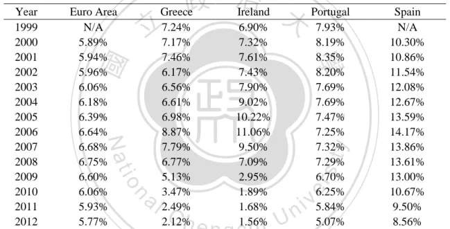
(20) 2. Monetary Policy and Real Estate Bubbles. 2.1. Introduction The four European countries 3 Greece, Ireland, Portugal and Spain stand in the epicentre of the current financial crisis in Europe. As for Ireland and Spain, there is broad consent that the housing market played an important role in putting them into financial distress. In the case of Greece and Portugal, the economic downturn was mainly associated with structural issues, high government spending as well as an. 政 治 大 differ across these countries, 立they share several characteristics.. inefficient administrative system. Although the roots of the ongoing Eurozone crisis. ‧ 國. 學. The most apparent similarity is that the economies of these four countries have become particularly weak in the course of the Eurozone crisis. Another important. ‧. similarity is that these four countries relied strongly, above Eurozone average, on the. Nat. sit. y. construction sector. The initial boom in the construction sector across most of these. n. al. er. io. countries came to an abrupt end when the real estate sector collapsed in the late 2008.. i n U. v. The economic downturn in the construction sector went hand in hand with falling. Ch. engchi. housing prices in Greece, Ireland and Spain right after the crisis followed by further massive price declines across all four countries at the end of 2012 (Igan & Loungani, 2012). Table 2.1 gives an overview of the gross value added (GVA) of the construction sector as a share of total GVA in the four countries relative to the Eurozone average. The data shows that the weight of the construction sector in all of the four countries. 3. Due to their relatively weak and unstable economy, these four countries were often referred to as “PIGS” countries in the discussion related to the ongoing financial crisis in Europe. Originally this acronym was used to describe the four south European countries Greece, Italy, Portugal and Spain. In the course of the outbreak of the European sovereign-debt crisis Ireland replaced Italy in the group of the so called “PIGS” countries.. 9.
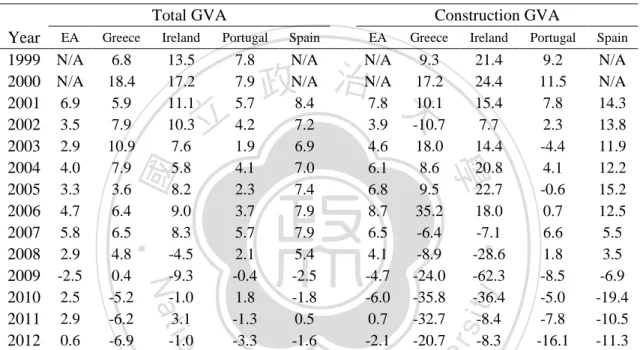
(21) was above the Eurozone average in the time period from the inception of the single monetary policy in the Eurozone in 19994 to the collapse in 2008. While the weight of the construction sector in Greece and Portugal was around 1-2% above the Eurozone average, Ireland displayed temporarily and Spain constantly values above 10%, putting them much above the Euro area average. In the extreme case of Spain, the size of the construction sector was for some time twice as large as the Eurozone average. This strong reliance on the construction sector made the economies of the four countries particularly vulnerable to the downturn in the housing market.. 政 治 大. Table 2.1: GVA of the Construction Industry as a Share of Total GVA Year Euro Area Greece Ireland Portugal Spain 1999 N/A 7.24% 6.90% 7.93% N/A 2000 5.89% 7.17% 7.32% 8.19% 10.30% 2001 5.94% 7.46% 7.61% 8.35% 10.86% 2002 5.96% 6.17% 7.43% 8.20% 11.54% 2003 6.06% 6.56% 7.90% 7.69% 12.08% 2004 6.18% 6.61% 9.02% 7.69% 12.67% 2005 6.39% 6.98% 10.22% 7.47% 13.59% 2006 6.64% 8.87% 11.06% 7.25% 14.17% 2007 6.68% 7.79% 9.50% 7.32% 13.86% 2008 6.75% 6.77% 7.09% 7.29% 13.61% 2009 6.60% 5.13% 2.95% 6.70% 13.00% 2010 6.06% 3.47% 1.89% 6.25% 10.67% 2011 5.93% 2.49% 1.68% 5.84% 9.50% 2012 5.77% 2.12% 1.56% 5.07% 8.56% Note: Data is sourced from the Eurostat database (Eurostat, 2013). Construction gross value added (GVA) is used instead of gross domestic product (GDP) because there are no GDP figures on individual economic sectors available. The GVA can be calculated as GDP+ subsidies- taxes on products. The ratio shown gives an indication on the size of the construction sector relative to the entire economy. *Euro Area (EA) country aggregate includes the countries which were part of the Eurozone at the respective point in time (EA112000, EA12-2006, EA13-2007, EA15-2008, EA16-2010, EA17).. 立. ‧. ‧ 國. 學. n. er. io. sit. y. Nat. al. Ch. engchi. i n U. v. Table 2.2 illustrates the Y-o-Y growth rate of the total and construction sector gross value added (GVA). The table emphasizes two central points. First, in the booming years, the economic growth in three of the four countries, namely Greece, Ireland and. 4. While Ireland, Portugal and Spain became part of the Eurozone on 01 January 1999, Greece was admitted two years later on 01 January 2001 as a member of the Eurozone.. 10.
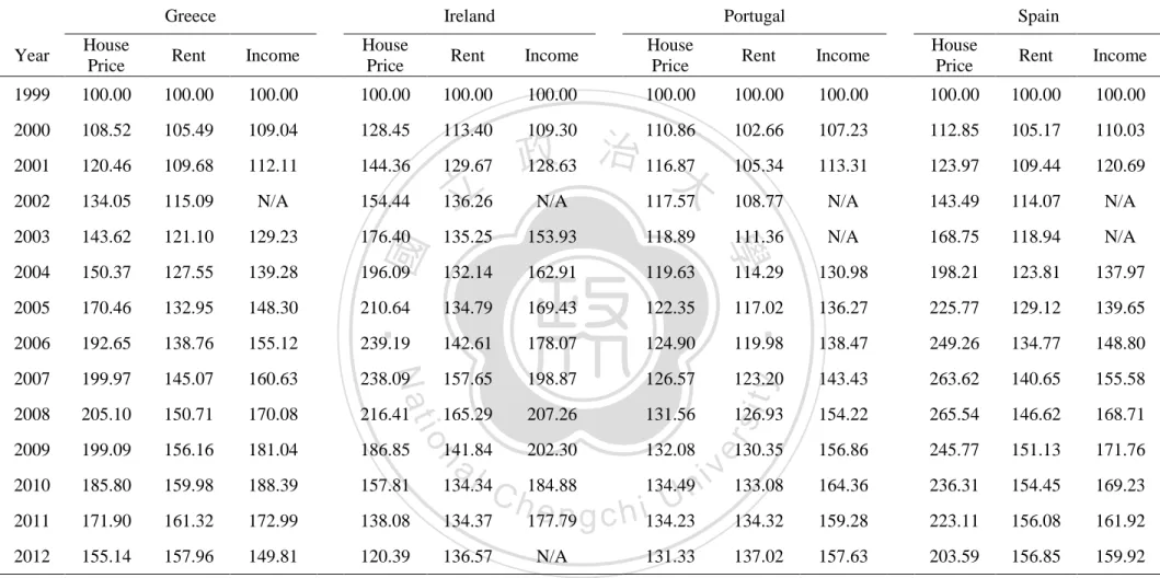
(22) Spain propelled the economy much faster than the Eurozone average as well as other sectors as indicated by Y-o-Y growth rates in the total GVA. Second, in the years after the collapse of the real estate sector, the construction sector in all of the four countries fell much faster than the Eurozone average. This sharp drop in the economic activity in the construction sector had a spillover effect on the economy as a whole, contributing strongly to the slowdown of the broad economy. Table 2.2: Y-o-Y Growth of Total GVA and Construction GVA Total GVA. Construction GVA. Ireland Portugal Spain Year 6.8 13.5 7.8 N/A N/A 9.3 21.4 9.2 N/A 1999 N/A 17.2 7.9 N/A N/A 17.2 24.4 11.5 N/A 2000 N/A 18.4 5.9 11.1 5.7 8.4 7.8 10.1 15.4 7.8 14.3 2001 6.9 7.9 10.3 4.2 7.2 3.9 -10.7 7.7 2.3 13.8 2002 3.5 10.9 7.6 1.9 6.9 4.6 18.0 14.4 -4.4 11.9 2003 2.9 7.9 5.8 4.1 7.0 6.1 8.6 20.8 4.1 12.2 2004 4.0 3.6 8.2 2.3 7.4 6.8 9.5 22.7 -0.6 15.2 2005 3.3 6.4 9.0 3.7 7.9 8.7 35.2 18.0 0.7 12.5 2006 4.7 6.5 8.3 5.7 7.9 6.5 -6.4 -7.1 6.6 5.5 2007 5.8 4.8 -4.5 2.1 5.4 4.1 -8.9 -28.6 1.8 3.5 2008 2.9 0.4 -9.3 -0.4 -2.5 -4.7 -24.0 -62.3 -8.5 -6.9 2009 -2.5 -5.2 -1.0 1.8 -1.8 -6.0 -35.8 -36.4 -5.0 -19.4 2010 2.5 -6.2 3.1 -1.3 0.5 0.7 -32.7 -8.4 -7.8 -10.5 2011 2.9 -6.9 -1.0 -3.3 -1.6 -2.1 -20.7 -8.3 -16.1 -11.3 2012 0.6 Note: Data is sourced from the Eurostat database (Eurostat, 2013). GDP and construction GVA Y-o-Y growth rates are calculated on the basis of the GDP and construction GVA at current market prices respectively. *Euro Area (EA) country aggregate includes the countries which were part of the Eurozone at the respective point in time (EA11-2000, EA12-2006, EA13-2007, EA15-2008, EA16-2010, EA17). EA. Greece. Ireland. Portugal. 立. Spain. EA. Greece. 政 治 大. ‧. ‧ 國. 學. n. er. io. sit. y. Nat. al. Ch. engchi. i n U. v. The booming years in Greece, Ireland and Spain went hand in hand with a strong increase in housing prices. On the contrary, not only Portugal’s construction industry grew much slower than the other countries but also its price. Particularly in the case of Ireland and Spain it has been often argued that these countries experienced price increases that cannot be explained by actual, consumption-driven, demand. In fact, as Table 2.3 shows, house prices in Greece, Ireland and Spain increased much faster than rent and income. 11.
(23) Table 2.3: House Prices, Rent and Income Greece. Ireland. Portugal. Spain. Year. House Price. Rent. Income. House Price. Rent. Income. House Price. Rent. Income. House Price. Rent. Income. 1999. 100.00. 100.00. 100.00. 100.00. 100.00. 100.00. 100.00. 100.00. 100.00. 100.00. 100.00. 100.00. 2000. 108.52. 105.49. 109.04. 128.45. 113.40. 109.30. 110.86. 102.66. 107.23. 112.85. 105.17. 110.03. 2001. 120.46. 109.68. 112.11. 144.36. 129.67. 105.34. 113.31. 123.97. 109.44. 120.69. 2002. 134.05. 115.09. N/A. 154.44. 136.26. 2003. 143.62. 121.10. 129.23. 176.40. 2004. 150.37. 127.55. 139.28. 2005. 170.46. 132.95. 2006. 192.65. 2007. 108.77. N/A. 143.49. 114.07. N/A. 135.25. 153.93. 118.89. 111.36. N/A. 168.75. 118.94. N/A. 196.09. 132.14. 162.91. 119.63. 114.29. 130.98. 198.21. 123.81. 137.97. 148.30. 210.64. 134.79. 169.43. 122.35. 117.02. 136.27. 225.77. 129.12. 139.65. 138.76. 155.12. 239.19. 142.61. 178.07. 124.90. 119.98. 138.47. 249.26. 134.77. 148.80. 199.97. 145.07. 160.63. 238.09. 157.65. 198.87. 126.57. 123.20. y. 143.43. 263.62. 140.65. 155.58. 2008. 205.10. 150.71. 170.08. 216.41. 165.29. 207.26. 131.56. 154.22. 265.54. 146.62. 168.71. 2009. 199.09. 156.16. 181.04. 186.85. 202.30. 132.08. 156.86. 245.77. 151.13. 171.76. 2010. 185.80. 159.98. 188.39. 157.81. 164.36. 236.31. 154.45. 169.23. 2011. 171.90. 161.32. 172.99. 138.08. 134.49n C h184.88 U e n g c h i134.23 134.37 177.79. i v 133.08 134.32. 159.28. 223.11. 156.08. 161.92. 2012. 155.14. 157.96. 149.81. 120.39. 136.57. 137.02. 157.63. 203.59. 156.85. 159.92. io. n. al. 134.34. N/A. 131.33. 126.93. er. Nat. 141.84. ‧. ‧ 國. 117.57. 學. N/A. sit. 立. 治 116.87 政 128.63 大. 130.35. Note: Data on housing prices is sourced from the property price database of the European Central Bank (ECB, 2013b) and the Bank for International Settlements (BIS, 2013b). Population and income data is sourced from the Eurostat database (Eurostat, 2013). Income is the figure on median equalized net income. To allow for comparability, the quarterly house price and rent indices are transformed to annual data by calculating the arithmetic average of the quarterly values of the respective year and all of the time series are further adjusted so that 1999=100.. 12.
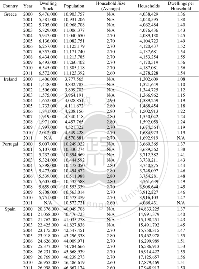
(24) Only in the case of Portugal, the development of the house price relative to rent and income was more balanced with fundamental factors. Relatively high owner occupancy rates 5 in all of the four countries further show a strong preference for buying versus renting (EMF, 2012), partially explaining the divergence between actual and investment demand. Looking at the supply side of residential housing further strengthens the point that the price increase, particularly in Greece, Ireland and Spain cannot be explained by actual, consumption-driven, demand. Table 2.4 provides an overview of the yearly. 治 政 大this table is calculated on the households. The key figure- dwelling per household, in 立 development of the total housing stock in the four countries relative to the number of. basis of the total dwelling stock and number of households in the respective country.. ‧ 國. 學. Thereby, a value below one indicates housing shortage and a figure above one. ‧. indicates oversupply. Two key observations can be attained on the basis of the figure. sit. y. Nat. on dwellings per household. First, all of the four countries display an oversupply in. io. al. er. housing. As of 2010, Greece shows the largest oversupply with 1.56 dwelling per household, followed by Spain with 1.51, Portugal with 1.47 and Ireland with 1.19.. n. v i n C h2.4 is further confirmed Table engchi U. The figure presented in. by figures on vacant. conventional dwellings as a percentage of total dwelling stock shown in a report on housing statistics in the European Union (Dol & Haffner, 2010). The report indicates vacancy rates of 33.2% for Greece in 2001, 21.9% for Spain in 2004, 10.6% for Portugal in 2001 and 12% for Ireland in 2002. Second, all of the four countries showed an upward trend in the dwellings per household, indicating a constantly increasing oversupply of housing.. 5. While the owner occupancy rate of the EU 27 average of the latest figures was at 68.9%, this rate stood in 2010 at 80.1% in Greece, 74.5% in Ireland and 74.9% in Portugal and in 2008 at 85% in Spain..
(25) Table 2.4: Total Dwelling Stock and Number of Households Dwelling Household Size Dwellings per Population Households Stock (Average) Household Greece 2000 5,476,000 10,903,757 N/A 4,038,429 1.36 2001 5,581,000 10,931,206 N/A 4,048,595 1.38 2002 5,705,000 10,968,708 N/A 4,062,484 1.40 2003 5,829,000 11,006,377 N/A 4,076,436 1.43 2004 5,947,000 11,040,650 2.70 4,089,130 1.45 2005 6,136,000 11,082,751 2.70 4,104,723 1.49 2006 6,257,000 11,125,179 2.70 4,120,437 1.52 2007 6,357,000 11,171,740 2.70 4,137,681 1.54 2008 6,434,000 11,213,785 2.70 4,153,254 1.55 2009 6,493,000 11,260,402 2.70 4,170,519 1.56 2010 6,545,000 11,305,118 2.70 4,187,081 1.56 2011 6,572,000 11,123,392 2.60 4,278,228 1.54 Ireland 2000 1,406,000 3,777,565 N/A 1,302,609 1.08 2001 1,448,000 3,832,783 N/A 1,321,649 1.10 2002 1,506,000 3,899,702 N/A 1,344,725 1.12 2003 1,575,000 3,964,191 N/A 1,366,962 1.15 2004 1,652,000 4,028,851 2.90 1,389,259 1.19 2005 1,733,000 4,111,672 2.80 1,468,454 1.18 2006 1,841,000 4,208,156 2.80 1,502,913 1.22 2007 1,919,000 4,340,118 2.80 1,550,042 1.24 2008 1,971,000 4,457,765 2.80 1,592,059 1.24 2009 1,997,000 4,521,322 2.70 1,674,564 1.19 2010 2,012,000 4,549,428 2.70 1,684,973 1.19 2011 N/A 4,570,881 2.70 1,692,919 N/A Portugal 2000 5,007,000 10,249,022 N/A 3,660,365 1.37 2001 5,107,000 10,330,774 N/A 3,689,562 1.38 2002 5,232,000 10,394,669 N/A 3,712,382 1.41 2003 5,324,000 10,444,592 N/A 3,730,211 1.43 2004 5,398,000 10,473,050 2.80 3,740,375 1.44 2005 5,473,000 10,494,672 2.80 3,748,097 1.46 2006 5,539,000 10,511,988 2.80 3,754,281 1.48 2007 5,603,000 10,532,588 2.80 3,761,639 1.49 2008 5,659,000 10,553,339 2.70 3,908,644 1.45 2009 5,708,000 10,563,014 2.70 3,912,227 1.46 2010 5,751,000 10,573,479 2.70 3,916,103 1.47 2011 N/A 10,572,721 2.60 4,066,431 N/A Spain 2000 20,376,000 40,049,708 N/A 14,833,225 1.37 2001 21,058,000 40,476,723 N/A 14,991,379 1.40 2002 21,762,000 41,035,278 N/A 15,198,251 1.43 2003 22,425,000 41,827,838 N/A 15,491,792 1.45 2004 23,175,000 42,547,451 2.70 15,758,315 1.47 2005 23,918,000 43,296,338 2.80 15,462,978 1.55 2006 24,626,000 44,009,971 2.70 16,299,989 1.51 2007 25,377,000 44,784,666 2.70 16,586,913 1.53 2008 26,231,000 45,668,939 2.70 16,914,422 1.55 2009 26,769,000 46,239,273 2.70 17,125,657 1.56 2010 26,953,000 46,486,619 2.60 17,879,469 1.51 2011 26,998,000 46,667,174 2.60 17,948,913 1.50 Note: Data on total dwelling stock and population as well as average household size is sourced from the European Mortgage Federation (EMF, 2012) and the Eurostat database (Eurostat, 2013) respectively. Prior to 2004, no data on average household size is available, thus the 2004 figure is used. Year. 立. 政 治 大. 學. ‧. ‧ 國. io. sit. y. Nat. n. al. er. Country. Ch. engchi. 14. i n U. v.
(26) Although the four countries experienced an increase in dwellings per household, housing prices, particularly in Greece, Ireland and Spain increased dramatically. This pattern indicates that the housing price increase in the four countries cannot be entirely explained by an increase in housing demand for living purpose. It rather indicates that the price increase in these countries throughout the observed period is investment driven. In response to the global financial and ongoing Eurozone crisis, it has been often pointed out that monetary policy plays a crucial role in the determination of asset. 治 政 大 out that money and credit price bubbles and monetary policy, the ECB (2010) pointed 立. price bubbles across different asset classes. For instance, in a general report on asset. indicators help to predict booms and busts cycles in asset prices. In regard to property. ‧ 國. 學. bubbles, a member of the Executive Board of the ECB stated that simple money and. ‧. credit aggregates deviations from a trend that exceeds a given threshold provide a. sit. y. Nat. useful predictor of costly boom and bust cycles (Praet, 2011). Another member of the. io. al. er. Executive Board of the ECB emphasized in a speech on Ireland that ballooning credit. n. and spending excesses overheated the economy and misdirected resources during the. Ch. booming years before the crisis (Asmussen, 2012).. engchi. i n U. v. The purpose of this essay is to address three questions. First, to what extent did Greece, Ireland, Portugal and Spain experience real estate bubbles in the period from entering the Eurozone and the end of 2012? Second, what is the role of the single monetary policy of the ECB in the formation of property bubbles in these countries? Third, why does the monetary policy of the ECB have a diverging effect on the formation of real estate bubbles in these countries? The rest of this essay is grouped into five parts. In the first part, the literature review gives a short overview on the literature on real estate bubble and the role of monetary policy in the formation of. 15.
(27) bubbles. The following two parts then move to the framework and data section. The framework draws from Stiglitz’s (1990) theory on asset bubbles and applies the direct capitalization approach through weighted average cost of capital (WACC) to identify real estate bubbles in the four countries. In the empirical part, Vector Autoregression (VAR) and Vector Error Correction (VEC) models are set up and impulse response analysis applied to investigate the relationship between the monetary policy of the ECB and property bubbles in the four countries. Finally, the findings from the analysis are discussed and a summary of the central arguments of this essay presented.. 2.2. Literature Review. 立. 政 治 大. 2.2.1. Real Estate Bubbles. ‧ 國. 學. The definition of a bubble is simple. A bubble describes the situation where the. ‧. market price is higher than the fundamental value or not justified by fundamental. sit. y. Nat. factors (Stiglitz, 1990). Although there is common consent about the definition of a. io. er. bubble, the measurement of the fundamental value is a difficult task. In the literature, there are several approaches on how to determine the fundamental value of real estate.. al. n. v i n C hin one approach from The fundamental value is derived e n g c h i U an equilibrium model and. usually contains a number of variables such as income, employment, construction cost and interest rates. For example, Hui and Yue (2006) applies a comparative study on housing price bubbles in Hong Kong, Beijing and Shanghai and uses disposable income, the stock of vacant new dwellings and local GDP as market fundamentals. Mikhed and Zemcik (2009) investigate whether the recently high and rapidly decreasing US house prices have been justified by fundamental factors. In their structural model of the housing market, personal income, population, house rent, stock market wealth, building costs, and mortgage rate are used as fundamentals.. 16.
(28) Another approach is the user cost framework developed by Poterba (1984). The key concept behind this framework is that individuals base their decision of owning or renting a house on the relative cost. Thereby the cost of owning a house is calculated by adjusting the house price by the user cost of housing6. Under the long-run housing market equilibrium, the cost of owning a house equals the cost of renting. Individuals adjust its consumption preference until the equilibrium is reached. For instance, if the cost of owning a house is high relative to the cost of renting it, house prices must fall or rents must rise to calibrate the market equilibrium. Related to the user cost. 治 政 大 The idea is that the the present value of the expected stream of future cash-flow. 立 approach of Poterba (1984) is the present-value approach. This approach focuses on. market is in equilibrium when the housing price equals the present value of the future. ‧ 國. 學. cash-flow. There are several studies applying different variations of this approach.. ‧. Many studies (Bjoerklund & Soederberg, 1999; Chan, Lee, & Woo, 2001; J. D.. sit. y. Nat. Hamilton, 1985; Hatzvi & Otto, 2008; Smith & Smith, 2006; Xiao & Tan, 2007). io. er. model the fundamental value as the sum of the expected rental income discounted at a. al. constant rate of return. Unlike the equilibrium model outlined above, this approach. n. v i n C h variables and U does not rely on other macroeconomic e n g c h i thus does not need a lot of data. Mikhed and Zemcik (2009) also focuses on the rent as determinant of the cash-flow associated with owning a house. In their analysis, however, the rent-to-price ratio is used to detect the discrepancy between fundamental and market value. Smith and Smith (2006) acknowledge that rental savings are the central factor determining the fundamental value of an owner-occupied home but they emphasize that other factors such as transaction costs, down payment, insurance, maintenance costs, property taxes, 6. Following Poterba (1984), the user cost of housing includes the foregone interest that the homeowner could have earned by investing in an alternative risk-free asset known as “opportunity cost”, the cost of property taxes, tax deductibility of mortgage interest and property taxes, maintenance cost, expected capital gain or loss and an additional risk premium to compensate homeowners of the higher risk of owning versus renting.. 17.
(29) mortgage payments, tax savings, and the proceeds if the home is sold at some point have an impact on the cash flow. Black et. al. present (2006) another variation of the present-value approach which is based on the present value of real disposable income to determine the fundamental value of housing. Another representation of the present-value approach is the state-space model which can be used to empirically estimate the size of housing bubbles. This time series model includes one or more unobservable (state) variables and represents its dynamics in a state equation. The model further consists of the observation equation. 治 政 大on the state-space model of variables. In a recent study, Teng et. al. (2013) build 立 that captures the relationship between the observed variables and unobserved. Alessandri (2006) on stock market and apply it to the context of real estate markets in. ‧ 國. 學. Taipei and Hong Kong. In their model, the state equation captures the movement of. ‧. the bubble and allows the bubble price to move at time varying rates determined by. sit. y. Nat. the bubble price and risk-free rate in the previous period. The observation equation. io. er. captures the market price and contains the rent, risk-free interest rate and the bubble. al. as unobservable component. The combination of these two equations form the state-. n. v i n C h the deviation ofUthe observed market price from space model which is used to separate engchi. the fundamental price into measurement error and the bubble price, whose evolution is driven by lagged bubble price and interest rate. The underlying concept of Teng et. al.’s (2013) state-space model is the same as the simple present-value framework. This state-space model is just another more sophisticated representation of the present-value approach which allows separating the deviation of the observed market price from the fundamental price into measurement error generated by a white noise process and the bubble price which is driven by lagged bubble price and interest rate. Instead of the state-space representation of the present-value approach, the following. 18.
(30) analysis applies a simple present-value approach that takes, through the weighted average cost of capital, financial leverage into account. This approach is used because it is widely applied by practitioners in real estate markets and can be readily understood by a broad audience. 2.2.2. Monetary Policy and Property Bubbles Several papers analyze the relationship between monetary policy variables and housing prices. For instance, Ahearne et. al. (2005) examine the rise and fall of real house prices since the 1970 in 18 major industrialized countries including Ireland and. 政 治 大 easing monetary policy. Another 立 recent study (Adams & Füss, 2010) applies panel Spain. The analysis shows that real house prices are typically preceded by a period of. ‧ 國. 學. cointegration analysis to a sample of 15 OECD countries, including Ireland and Spain, over the period of 30 years to study the macroeconomic determinants of international. ‧. housing markets. The analysis shows that besides the economic activity and. Nat. sit. y. construction cost, the long-term interest rate also has a significant inverse impact on. al. n. 1% level.. er. io. housing prices. As for Ireland and Spain, this inverse relationship is significant at the. Ch. engchi. i n U. v. There are also several studies in the literature specifically looking at the relationship between monetary policy variables and housing bubbles. In this regard, Tsai and Peng (2011) analyze house prices in four cities in Taiwan. The empirical result of the panel unit root and cointegration test shows that bubble-like behavior of house prices in Taiwan after 1999 was primarily related to the mortgage rates. The study concludes that expansionary monetary policy, which leads to speculations and lower mortgage rates, is the key driver for housing bubbles. Another study (Agnello & Schuknecht, 2011) looks into the determinants of housing market booms and busts in eighteen industrialized countries, including Ireland and Spain, from 1980 to 2007. The 19.
(31) estimates from the multinomial probit model indicate that domestic credit and interest rates have a significant impact on the probability of booms and busts. The evidence indicates that regulatory policies which slow down money and credit growth reduce boom probabilities. Confrey and Gerald (2010) show with the example of Ireland and Spain that the introduction of the single monetary policy under the ECB and its monetary policy was a main factor causing real estate bubbles in the booming periods. Specifically, the analysis points out that the regime change brought about a substantial reduction in the. 治 政 大in turn supported households and Spain, the reduction was particularly strong which 立 real cost of capital for households in many Eurozone countries. In the case of Ireland. in these countries to finance their investment in the housing market. The regime. ‧ 國. 學. change not only lowered the real cost of capital but also made it much easier for the. sit. y. Nat. of households.. ‧. domestic financial system in Ireland and Spain to fund the dramatic investment surge. io. er. In sum, monetary policy variables play a crucial role in the rise of real estate prices. al. and the formation of bubbles. This study contributes to this literature by analyzing the. n. v i n relationship between the bubbleC formation Ireland, Portugal and Spain and h e n gin cGreece, hi U the monetary policy of the ECB, the top authority controlling money supply and key interest rates in the European monetary union. This essay further sheds light on the reasons of diverging bubble formation across these countries.. 2.3. Framework 2.3.1. Property Bubble Determination An asset bubble, as defined by Stiglitz (1990), describes the situation where only investor’s expectations of higher selling prices instead of the fundamental factors. 20.
(32) determine the high price today. In such a situation, investors ignore the fundamental value and bid prices up, assuming that other investors will push prices further. The bubble is created by a form of speculation which does not rely on future income streams but on expected bullish behavior of other investors. Such a situation is inherently unstable and referred to as the greater fool theory of investing. As soon as the pool of greater fools dries up, the market turns bearish and corrects towards its fundamental value. Accordingly, an asset bubble exists when the market price (MV) is higher than the fundamental value (FV). MV >. (1) 治 政 While it is simple to identify the market price, it is a大 difficult task to determine the 立 fundamental value. As discussed in the literature review, there are several approaches. ‧ 國. 學. to determine the fundamental value. This essay applies the present-value approach to. ‧. determine the fundamental value. In this case, the fundamental value is determined by. sit. y. Nat. the present value of the anticipated cash flow from the property investment (Mikhed. io. er. & Zemcik, 2009). A real estate investor receives rent payments and will make a profit. al. or loss from selling the house. Consequently, the fundamental value should be close. n. v i n C h discounted backUby the required rate of return. to the flow of future rent payments engchi Although the rent is the central factor in the calculation of the cash-flow, there are also other variables which affect the future flow of payments as transaction costs, insurance, maintenance costs, property taxes and tax savings (Smith & Smith, 2006). Due to data availability and simplicity, however, the fundamental value is treated as the discounted future rent. Most present-value models apply a constant discount rate; however, it is crucial to use the appropriate modelling of the discount rate or else a bubble could be identified when in fact, there is no discrepancy between the market and fundamental value (Black et al., 2006). Hence this study applies a time-varying. 21.
(33) discount rate. Furthermore, most studies using present-value models employ a riskfree rate of return, i.e. long-term yields of government bonds, as a proxy for the required rate of return. In practice, however, most residential properties in the Euro area are bought by individual investors financing their property via mortgage loans (ECB, 2009). The concept of weighted average cost of capital (WACC) 7 allows considering this feature by incorporating both the cost of equity and debt. The loan-tovalue ratio (L/V) adjusts the proportion of the cost of debt (i. ) and equity (i ). which is used to finance the house purchase. The subscript j is for the country and t. 政 治 大 year at a domestic bank as the opportunity cost of equity and the average interest rate 立 for the time. The average interest rate for deposits with agreed maturity of up to 1. 學. ‧ 國. for house purchase as the cost of debt are used. The following analysis assumes that the typical loan-to-value ratio is 0.78. ×i. +. 1−. ×i. ‧. WACC =. (2). Nat. sit. y. The fundamental value of residential real estate is the rent discounted by the WACC.. n. al. er. io. In the following definition FV is the fundamental value, RENT the rent, and WACC the weighted average cost of capital.. Ch. e n g!"c h i. FV = %&''#$. i n U. #$. v. (3). Referring back to formula (1), a positive property bubble exists when the market price of real estate is higher than the fundamental value. Thus, the bubble in percentage terms is calculated as following. ()* = +. , #$ - . #$ / . #$. × 100. (4). A positive bubble indicates that the market price is higher than the fundamental value and vice versa. 7 8. For simplicity, other factors, such as risk premium are not considered in the calculation of the WACC. The data section shows a simulation of the bubble under five different LTV scenarios.. 22.
(34) 2.3.2. Monetary Policy Transmission Real estate bubbles are basically linked to monetary policy through two different channels. First, house prices are sensitive to the interest rate on other financial assets such as bonds or deposits at a bank. Zeno and Füss (2010) point out that increasing long-term interest rates do not change the actual demand for housing space directly but rather change the investment demand for housing. An increase in the policy interest rate increases the return on other fixed-income assets relative to the return of real estate; hence it shifts the demand away from real estate into other assets. The. 治 政 大actual need for housing for provide incentives for real estate investment. While the 立. opposite holds true for low interest rates which reduce the return on equity and thus. living purpose remains the same, the investment demand goes up and artificially. ‧ 國. 學. drives up the demand for residential real estate and housing prices.. ‧. Second, interest rates and money supply affect the debt financing conditions of. sit. y. Nat. borrowers. As pointed out by Zeno and Füss (2010), an increase in long-term interest. io. er. rate is reflected in higher mortgage rates, which reduces the demand for real estate.. al. On the opposite, low interest rates reduce the cost of mortgage loans, which increases. n. v i n the availability and accessibilityC toh house purchasing loans e n g c h i U and thus demand.. The interplay of both channels increases the demand for housing relative to the demand for rental housing. The unbalanced development of the demand in the two markets manifests, in a widening gap, between the market and fundamental value. The simplified relationship between property bubbles and the two channels of monetary policy can be expressed as following. ()* = 1(34* , 67* ). (5). This expression shows that the bubble ()* is a function of the interest rate 34* and the lending for house purchase-to-GDP 67* . In this case, the interest rate reflects both 23.
(35) interest rates on equity, i.e. returns gained from alternative financial assets such as bonds or deposits at a bank, as well as debt, i.e. mortgage rate. In order to approximate the interest rate effect on the bubble, this analysis applies the 3-month Euribor (Euro Interbank Offered Rate) which proxies the key interest rate set by the ECB. Hereby, the main refinancing operation is the most important monetary policy tool of the ECB. It provides liquidity through the national central banks to the domestic banking system in the member states of the Eurozone. The interest rate for this instrument is set in a tender procedure where the domestic banks make a bid and. 治 政 大the transaction is completed, loan and provide financial assets as a guarantee. After 立. receive a short-term loan with maturity of one week. The domestic banks receive the. the domestic banks pay interests to the central bank and receive the provided. ‧ 國. 學. collateral in return. The interest rate set in the tender procedure is subject to a. ‧. minimum bid rate. The minimum bid rate is set on a monthly basis by the Governing. sit. y. Nat. Council of the ECB. In the tender procedure, the total amount of funds to be allocated. io. er. is defined by the ECB. Domestic banks that make the highest bid are served first until. al. the full amount is allocated. Domestic banks unable to obtain liquidity through this. n. v i n Cinhthe money market.UMoney market interest rates as mechanism have to borrow funds engchi. the 3-month Euribor are usually very close to the minimum bid rate of the main refinancing operations set by the ECB (ECB, 2013a). The loan-to- GDP ratio is commonly used as a measure of bank lending activities (Oikarinen, 2009). Based on the theory of the two channels above, it is suggested that 34* is negatively and 67* positively related to the bubble in the short-run. In the long-run, however, the relationship between the bubble and 34* might be positive. This is because the longrun low interest rate may enhance investors’ confidence in housing investment, and consequently bolster the housing prices as well as the bubble.. 24.
(36) In the empirical part, VAR and VEC models are applied to analyze dynamics between the bubble, Euribor and the lending for house purchase-to-GDP ratio.. 2.4. Data For Ireland, Portugal and Spain, the analysis covers the time period from the inception of the single monetary policy in the Eurozone in 1999 to the third quarter of 2012. As Greece entered the Eurozone two years later, the analysis starts in 2001. As for the house price, price indices on residential property from the property price database of the ECB and the Bank for International Settlements (BIS) are used. In the. 政 治 大. case of Ireland, there is no complete time series on house prices for the entire period. 立. available. In order to cover the full time period, two overlapping time series are. ‧ 國. 學. consolidated into a single item. The rent index is sourced from the ECB and available. ‧. for the entire period. For the calculation of the WACC, due to data availability, data from two separate data sets is used. Historical quarterly data on retail interest rates is. y. Nat. er. io. sit. sourced from Eurostat and covers the time period from 1999 to 2003. The second data set is sourced from the Monetary Financial Institute (MFI) database from the ECB. n. al. Ch. i n U. v. and covers the period from 2003 to 2012. In order to allow the analysis of the full. engchi. time period, both data sets are consolidated. As for the cost of debt, the average interest rate for housing loans is used. Regarding the cost of equity, the average interest rate on deposits of up to one-year maturity is used. For Ireland, the average rate for overnight deposits is used as a proxy for the cost of equity as the previously mentioned interest is not available for this country. The data on the Euribor and the lending for house purchase-to-GDP is also sourced from Eurostat and available for the entire period.. 25.
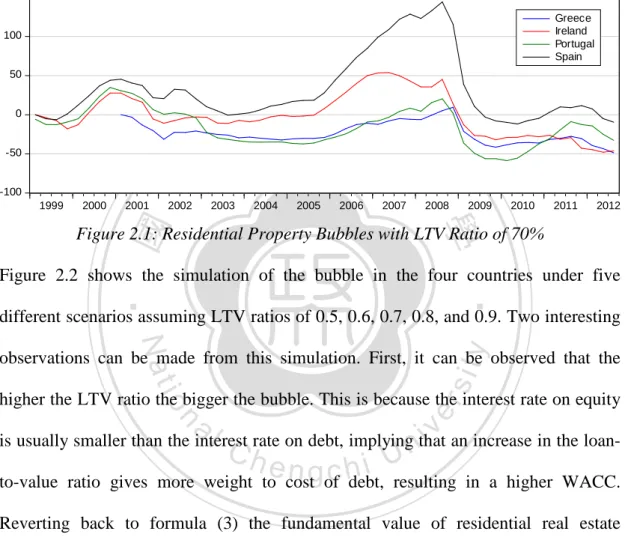
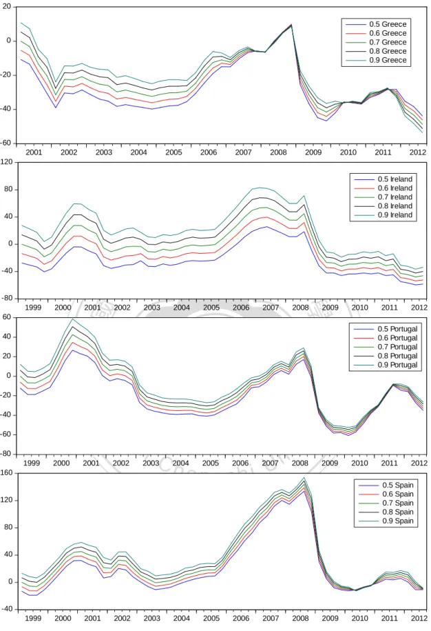
(37) The following figure shows the bubble 9 in the four countries according to the definition in (4). Ireland, Portugal and Spain experienced an increase in the bubble at the beginning of the 2000s, followed by a decrease up to 2005 in Portugal and a returning upward trend in Ireland and Spain in 2003. After a sharp drop in 2001, the bubble in Greece developed steadily before increasing at the end of 2005. 150 Greece Ireland Portugal Spain. 100. 50. 0. 政 治 大. -50. 立. -100 2000. 2001. 2002. 2003. 2004. 2005. 2006. 2007. 2008. 2009. 2010. 2011. 2012. 學. ‧ 國. 1999. Figure 2.1: Residential Property Bubbles with LTV Ratio of 70% Figure 2.2 shows the simulation of the bubble in the four countries under five. ‧. different scenarios assuming LTV ratios of 0.5, 0.6, 0.7, 0.8, and 0.9. Two interesting. y. Nat. io. sit. observations can be made from this simulation. First, it can be observed that the. n. al. er. higher the LTV ratio the bigger the bubble. This is because the interest rate on equity. Ch. i n U. v. is usually smaller than the interest rate on debt, implying that an increase in the loan-. engchi. to-value ratio gives more weight to cost of debt, resulting in a higher WACC. Reverting back to formula (3) the fundamental value of residential real estate decreases when the WACC increases. Hence the bubble increases with an increase in the WACC.. 9. The starting value of the rent has been adjusted so that fundamental value equals the market value in the base period. The base period is set according to the point when the respective country entered the Eurozone. Therefore, the base period is 2001Q1 in the case of Greece and 1999Q1 for the other countries. This adjustment does not imply that the fundamental value is equal to the fundamental value in the base period; it rather defines the respective year as the reference point. What matters in the subsequent analysis is the movement or the trend of the bubble.. 26.
(38) 20 0.5 Greece 0.6 Greece 0.7 Greece 0.8 Greece 0.9 Greece. 0. -20. -40. -60. 2001. 2002. 2003. 2004. 2005. 2006. 2007. 2008. 2009. 2010. 2011. 2012. 120 0.5 Ireland 0.6 Ireland 0.7 Ireland 0.8 Ireland 0.9 Ireland. 80. 40. 政 治 大. 0. 立. -40. 2000. 40. 0. 2002. 2003. 2004. 2005. 2006. 2007. 2008. al. n. -80. 1999. 2000. 2001. 2002. 160. 2012. 0.5 Portugal 0.6 Portugal 0.7 Portugal 0.8 Portugal 0.9 Portugal. sit. io. -60. 2011. er. -40. 2010. y. Nat. -20. 2009. ‧. 20. 2001. 學. 1999. 60. ‧ 國. -80. Ch. 2003. 2004. 2005. 2006. engchi. i n U. 2007. v. 2008. 2009. 2010. 2011. 2012. 0.5 Spain 0.6 Spain 0.7 Spain 0.8 Spain 0.9 Spain. 120. 80. 40. 0. -40 1999. 2000. 2001. 2002. 2003. 2004. 2005. 2006. 2007. 2008. 2009. 2010. 2011. Figure 2.2: Residential Property Bubble Simulation under Varying LTV Ratios. 27. 2012.
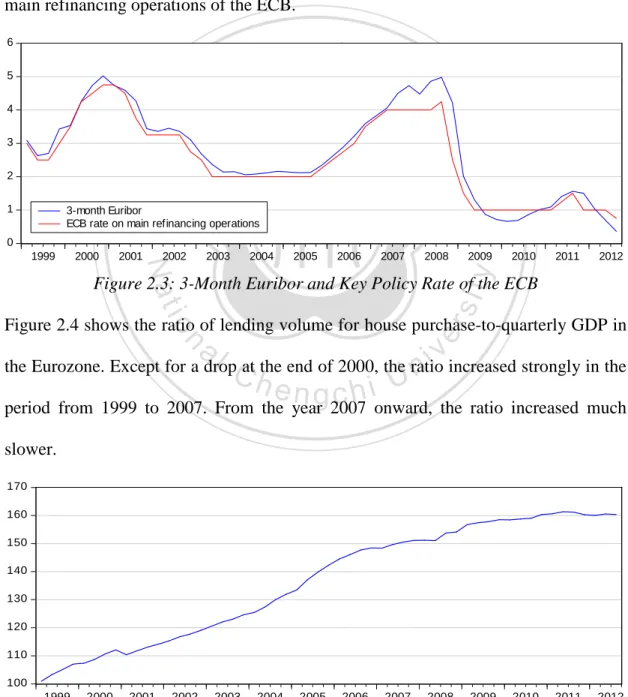
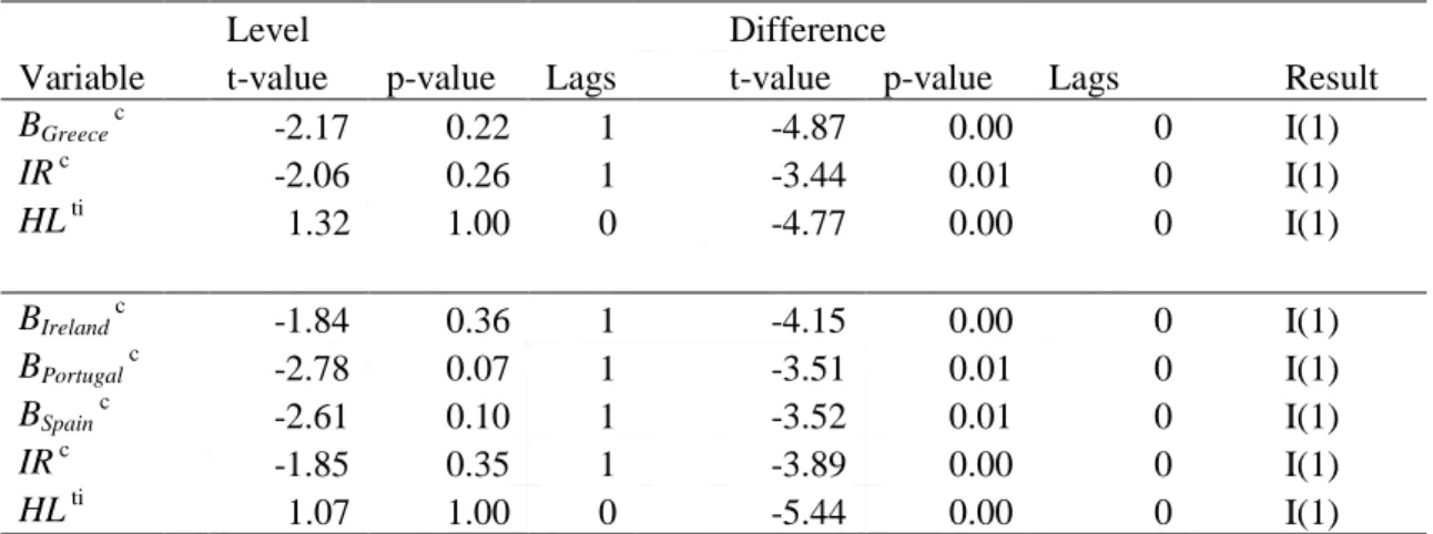
(39) Second, the trend of the bubble does not change with an adjustment of the loan-tovalue ratio. This point is important because the subsequent analysis builds on the movement or trend of the bubble rather than its absolute value. Figure 2.3 compares the minimum bid rate for main refinancing operations set by the ECB with the 3-month Euribor money market interest rate. It is obvious that the money market rate is closely related to the key interest rate of the ECB. In the subsequent analysis the 3-month Euribor is used as proxy for the interest rate on the main refinancing operations of the ECB.. 政 治 大. 6 5. 立. 4. ‧ 國. 學. 3 2 1. 2000. 2001. 2002. Nat. 1999. 2003. 2004. 2005. 2006. 2007. 2008. 2009. 2010. 2011. 2012. y. 0. ‧. 3-month Euribor ECB rate on main refinancing operations. io. sit. Figure 2.3: 3-Month Euribor and Key Policy Rate of the ECB. n. al. er. Figure 2.4 shows the ratio of lending volume for house purchase-to-quarterly GDP in. Ch. i n U. v. the Eurozone. Except for a drop at the end of 2000, the ratio increased strongly in the. engchi. period from 1999 to 2007. From the year 2007 onward, the ratio increased much slower. 170. 160 150 140 130 120 110 100 1999. 2000. 2001. 2002. 2003. 2004. 2005. 2006. 2007. 2008. 2009. 2010. 2011. Figure 2.4: Lending for House Purchase-to-Quarterly GDP in the Eurozone 28. 2012.
(40) In order to select the appropriate model for the following analysis, the augmented Dickey and Fuller (1979) (ADF) test is applied to determine the order of integration of the variables. A variable is said to be integrated of order n when it achieves stationarity after taking its n-th difference. As shown in Table 2.5, the ADF test statistic indicates at a significance level of 10% that all of the variables in its level contain a unit root. Table 2.5: ADF Unit Root Tests Variable BGreece c IR c HL ti. Level t-value p-value Lags -2.17 0.22 1 -2.06 0.26 1 1.32 1.00 0. Difference t-value p-value Lags -4.87 0.00 0 -3.44 0.01 0 -4.77 0.00 0. 政 治 大. 立. Result I(1) I(1) I(1). ‧. ‧ 國. 學. BIreland c -1.84 0.36 1 -4.15 0.00 0 I(1) BPortugal c -2.78 0.07 1 -3.51 0.01 0 I(1) BSpain c -2.61 0.10 1 -3.52 0.01 0 I(1) c IR -1.85 0.35 1 -3.89 0.00 0 I(1) HL ti 1.07 1.00 0 -5.44 0.00 0 I(1) Note: The results of the upper and lower panel are based on data covering the period from 2001Q1 to 2012Q3 and 1999Q1 to 2012Q3 respectively. The number of lags included in the ADF test is decided by the automatic lag length selection criteria based on SIC with maximum lag length of 10. c indicates that a constant term and ti indicates that a constant term as well as a linear time trend have been included in the model.. n. er. io. sit. y. Nat. al. Ch. i n U. v. The test further indicates that the first difference of all variables is stationary at the. engchi. same level of significance. Thus it can be concluded that all of the variables are integrated of order one, or I(1).. 2.5. Empirical Analysis 2.5.1. Long-Run Dynamics Engle and Granger (1987) show that a linear combination of two or more nonstationary variables may be stationary. Such a linear combination of non-stationary variables is referred to as cointegration. Following the definition, the components of the vector 8* = [8:* , 8;* , … , 8=* ]′ are said to be cointegrated if all components of 8* 29.
(41) are I(1) and a vector @ = [@: , @; , … , @= ]′ exists such that the linear combination @′8* = @: 8:* + @; 8;* + … + @= 8=* is stationary, or I(0). The stationary linear combination is the cointegration equation and may be interpreted as the long-run relationship among the variables in the model. To test for cointegration amongst the variables in each system the Johansen Methodology illustrated by Enders (2010) is applied. In the first step, undifferenced data is used and a separate VAR model for each country estimated to determine the appropriate maximum lag length of the respective model. Each VAR model includes. 政 治 大 on the basis of the sequential modified LR test statistic. Including four lags in the lag 立. three variables- the respective bubble, IR and HL. The maximum lag length is chosen. specification, the tests indicate a lag length of two for Portugal and four for Greece,. ‧ 國. 學. Ireland and Spain.. ‧. In the next step the third model considered by Johansen (1995) is estimated to. sit. y. Nat. determine the rank of integration. This model allows the time series to have linear. io. er. deterministic trends and includes an intercept but no trend in the cointegration. al. equation. The cointegration vector in this model removes the linear deterministic. n. v i n C h the unit roots soUthat the cointegration equation trend of the time series as it removes engchi. does not contain any trend. A cointegration equation without a linear trend is close to the idea of the cointegrating vector defining an equilibrium relationship. There are two possible test statistics, considering different alternative hypotheses, to determine the number of cointegration relationships, i.e. the rank of cointegration (r). Table 2.6 presents the corresponding results. Both test statistics indicate on a significance level of 5% that the variables in the model of Greece, Ireland and Spain are cointegrated of order one. In the case of Portugal, neither the Trace nor the Maximum-Eigenvalue test statistics show. 30.
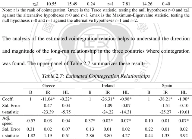
(42) cointegration. Thus, it can be concluded that there is a long-run relationship between the bubble and the two variables representing monetary policy in Greece, Ireland and Spain. In the case of Portugal, however, the results do not indicate such relationship. Table 2.6: Johansen Cointegration Tests Trace Test Country. Lag. H0. Maximum-Eigenvalue Test. 5% critical value. λtrace. pValue. H0. 5% critical value. λmax. pValue. Result. r=0 33.35 29.80 0.02 r=0 22.04 21.13 0.04 r=1 r≤1 11.31 15.49 0.19 r=1 6.47 14.26 0.55 Ireland 4 r=0 60.54 29.80 0.00 r=0 46.17 21.13 0.00 r=1 r≤1 14.37 15.49 0.07 r=1 10.83 14.26 0.16 Portugal 2 r=0 19.93 29.80 0.43 r=0 13.89 21.13 0.37 r=0 r≤1 6.04 15.49 0.69 r=1 4.30 14.26 0.83 Spain 4 r=0 36.26 29.80 0.01 r=0 25.71 21.13 0.01 r=1 r≤1 10.55 15.49 0.24 r=1 7.81 14.26 0.40 Note: r is the rank of cointegration. λtrace is the Trace statistic, testing the null hypotheses r=0 and r≤1 against the alternative hypotheses r>0 and r>1. λmax is the Maximum-Eigenvalue statistic, testing the null hypothesis r=0 and r=1 against the alternative hypotheses r=1 and r=2. Greece. 4. 政 治 大. 立. ‧ 國. 學. The analysis of the estimated cointegration relation helps to understand the direction. ‧. and magnitude of the long-run relationship in the three countries where cointegration. y. Nat. sit. was found. The upper panel of Table 2.7 summarizes these results.. al. n. B 1. Greece IR -11.04* 0.47 -23.39. Ch. HL -0.22* 0.04 -5.75. Ireland IR -26.31* -1.09 -24.22. B 1. engchi. er. io. Table 2.7: Estimated Cointegration Relationships. i n U HL -0.98* -0.07 -14.31. v. B 1. Spain IR -38.21* -1.51 -25.27. HL -1.90* -0.10 -19.61. Coeff. Std. Error t-statistic Adj. -0.57 0.03 0.04 0.37* 0.02* 0.07* 0.10 0.01 0.07* speed Std. Error 0.31 0.02 0.07 0.13 0.01 0.02 0.22 0.01 0.02 t-statistic -1.82 1.19 0.61 2.86 3.80 4.27 0.44 1.33 3.92 Note: * denotes significance at the 95% confidence interval. The critical value for the t-test is 1.96. Coeff. is the normalized cointegration coefficient; Adj. speed is the speed-of-adjustment coefficient and Std. error the respective standard error.. The normalized cointegration coefficients of the Euribor and the bubble indicate a significant positive relationship in all of the three countries. As already pointed out in the framework, the long-run relationship between the interest rate and the bubble. 31.
(43) might be positive. One possible explanation for this is that the long-run low interest rate enhances investors’ confidence in housing investment and consequently bolsters the housing prices as well as the bubble. The relationship between HL and the bubble is also significantly positive in all three countries. 2.5.2. Short-Run Dynamics In the next step, the short-run dynamics between the variables in the models are analyzed. In the case of Portugal, the Johansen cointegration test indicates no cointegration relationship. Therefore, a VAR model in first differences as specified. 政 治 大 is the 3×1 vector of intercept 立terms, A the 3×3 matrix of coefficients and ε the 3×1. below is set up. 8* is the 3×1 vector of the three variables included in the model. AB C. ‧ 國. 學. vector of error terms.. ∆8* = AB + A: ∆8*-: + ⋯ + AG ∆8*-G + ε. (6). ‧. In the case of Greece, Ireland and Spain, the same model is used for the Johansen. Nat. sit. y. cointegration test. The model includes a constant but no trend in the cointegration. n. al. er. io. vector. This model removes the linear deterministic trend of the time series as it. i n U. v. removes the unit roots so that the cointegration equation does not contain any trend.. Ch. engchi. This specification is close to the idea of the cointegrating equation defining an equilibrium relationship. The model is specified below where 8* is the 3×1 vector of the variables included in the model, AB is a 3×1 vector of constant terms, (@B + @ H I*-: ) the cointegrating equation, J the speed of adjustment, AC the 3×3 matrix of coefficients and ε the 3×1 vector of error terms. ∆8* = AB + J(@B + @ H 8*-: ) + A: ∆8*-: + ⋯ + AG-: ∆8*-GK: + ε. (7). The speed-of-adjustment coefficient indicates how the variables adjust to any discrepancies from the long-run equilibrium relationship. Given the positive value of the cointegrating equation, a positive coefficient indicates that the variable will go up 32.
(44) and a negative coefficient indicates that the variable will decrease. The lower panel of Table 2.7 shows the estimates. In the short-run, the bubble in Ireland responds with an increase and the bubble in Greece with a decrease to a deviation from the long-run equilibrium; the implication is that in the short-run the bubble tends to depart from the long-run equilibrium in Ireland but tends to approach the long-run equilibrium in Greece. In the case of Spain, the speed-of-adjustment coefficient is not significant at the 5% level of significance. Based on the VAR model for Portugal and the VEC model for the other three. 治 政 lending for house purchase-to-GDP and the bubble大 are analyzed by computing 立 countries, the dynamic effects of innovations in the money market interest rate and. orthogonalized impulse responses. Hereby the standard Choleski decomposition (C.. ‧ 國. 學. Sims, 1980) is used to derive the impulse responses. The ordering used is B-HL-IR. ‧. and aligned to the specification used by Hofmann (2004) and Oikarinen (2009).. sit. y. Nat. Following the ordering, it is assumed that the bubble does not respond instantly to. io. er. innovations in lending for house purchase-to-GDP and the Euribor. The lending for. al. house purchase does not respond instantly to a shock in the interest rate, and the. n. v i n C h the ECB and theU domestic banking system can interest rate is rather flexible because engchi. respond immediately with an interest rate change to alterations of the former two variables. Thus, the bubble may be affected within a quarter by the other two variables. The chosen ordering of the variables is common in the literature on monetary policy transmission and reflects the assumption that interest rate changes are transmitted to the economy with a lag. The following figures (Figure 2.5, Figure 2.6, Figure 2.7, Figure 2.8) illustrate the impulse responses up to 20 quarters from the shock. As outlined above, differenced data is used in the case of Portugal and data in. 33.
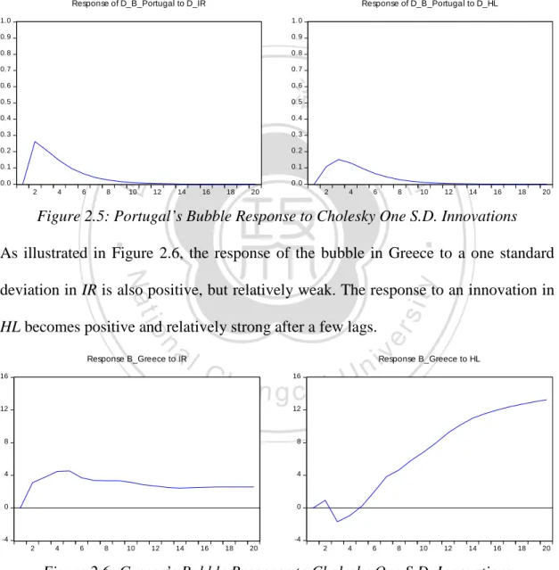
數據
+7
相關文件
6 《中論·觀因緣品》,《佛藏要籍選刊》第 9 冊,上海古籍出版社 1994 年版,第 1
The first row shows the eyespot with white inner ring, black middle ring, and yellow outer ring in Bicyclus anynana.. The second row provides the eyespot with black inner ring
• helps teachers collect learning evidence to provide timely feedback & refine teaching strategies.. AaL • engages students in reflecting on & monitoring their progress
Robinson Crusoe is an Englishman from the 1) t_______ of York in the seventeenth century, the youngest son of a merchant of German origin. This trip is financially successful,
fostering independent application of reading strategies Strategy 7: Provide opportunities for students to track, reflect on, and share their learning progress (destination). •
Although Taiwan stipulates explicit regulations governing the requirements for organic production process, certification management, and the penalties for organic agricultural
Estimated resident population by age and sex in statistical local areas, New South Wales, June 1990 (No. Canberra, Australian Capital
First Taiwan Geometry Symposium, NCTS South () The Isoperimetric Problem in the Heisenberg group Hn November 20, 2010 13 / 44.. The Euclidean Isoperimetric Problem... The proof
