TO-SALES RATIO WITH RESPECT TO CAPACITY UTILIZATION
Post script
YA-YEN SUNa* AND KAM-FAI WONGb
aDepartment of Kinesiology, Health and Leisure Studies, National University of Kaohsiung, Kaohsiung City, Taiwan; bInstitute of Statistics, National University of Kaohsiung,
Kaohsiung City, Taiwan
(Received 27 February 2010; In final form 18 September 2010)
Sun, Y-Y. & Wong, K-F. (2010). An important factor in job estimation: A nonlinear jobs-to-sales ratio with respect to capacity utilization. Economic Systems Research. 22(4), 427-446.
ABSTRACT
Many tools for economic impact evaluation, such as input-output models and computable general equilibrium models, rely on the jobs-to-sales ratio (JSR) to convert direct, indirect and induced effects of sales of final products into employment. For service sectors, this ratio is strongly influenced by capacity utilization and exhibits a non-linear pattern, especially for short-term tourism applications that involve dramatic demand fluctuations as a consequence of mega events, natural disasters or societal instability. The purpose of this study is to decompose the relationship between capacity utilization and the JSR so that the underlying factors which cause the instability of JSR can be identified. Time-series data from the Taiwanese tourist hotels and aviation sectors are adopted to discuss the strength of the relations between price per unit and capacity utilization, total employee numbers and utilization, service capacity and utilization, and labor efficiency and utilization, respectively. The main factor leading to changing JSRs is the inelasticity of the total employee number.
Keywords: capacity utilization, jobs-to-sales ratio, accommodation sector, aviation sector, Input-Output analysis
1. Introduction
Economic impacts analysis is frequently used in the tourism industry for policy evaluation, scenario comparisons and documentation of the contribution of tourism to regional economies. Most economic impacts studies evaluate spending changes, as induced by recreation activities or private/public investment. Next to figures on sales, impact studies often present indicators that are appealing to the general public and useful for policy evaluation. These indicators include employment, personal income, value added and government tax receipts. Among these indicators, job figures are generally perceived as the key measure for evaluation purposes (Gasparino et al., 2008). The absolute number of job opportunities and changes in the allocation of employment across industries caused by tourism are often used as a basis in decision-making regarding resource allocation and regional development.
To evaluate the employment effects associated with visitor expenditures or public/ private investment related to tourism, we generally rely on Input-Output analysis (IO) or Computer General Equilibrium models (CGE). The underlying principle of both models in calculating job impacts revolves around three factors: final demand change, regional sales multipliers and the jobs-to-sales ratio (JSR). The first factor, final demand change, specifies the total amount of money injected; regional sales multipliers indicate the structure of the local economy, representing the production function and the inter-industry linkages for the specified area during a given time period. The last factor, the jobs-to-sales ratio, characterizes the average ratio of labor inputs to production by each industry, which converts gross output changes, measured in dollar terms, into changes in employment. The accuracy of employment estimations jointly rests on these three components.
changes, economies of scale, as well as short-run price effects and supply constraints are assumed to have no influence on production coefficients (Miller & Blair, 1985; Rose & Miernyk, 1989; West, 1995). Based on these assumptions, an IO model presents a linear relationship between final demand changes and total economic impacts. For tourism applications, the adoption of stable IO multipliers call for special attention, since the IO model is frequently applied to evaluate large scale, irregular or unexpected tourism demand conditions. For “one-time” mega festivals or events such as the Olympic Games or FIFA World Cups, the predicted economic impacts of tourist expenditures on sales, jobs and personal income is often one of the driving factors to fight for the right to host the game (Ahlert, 2001; Lee & Taylor, 2005; Price Water House Coopers, 2005; Toohey & Veal, 2007). If large scale tourism crises emerge due to extreme natural disasters, disease outbreaks or terrorist activities (such as the SARS pandemic, the foot-mouth disease, or the 9/11 attacks), estimations of economic losses and job reductions in the tourism industry are very often used by governments to design recovery policies (Blake & Sinclair, 2003; Blake et al., 2003; Yang & Chen, 2009). A common feature of these events and situations is that they create substantial high/low demand patterns for fixed supply capacities in a region during a short-time period, ranging from a few days to a couple of months. To face such short-run demand fluctuations, businesses may adjust their production functions, which yields changes in the required intermediate inputs, labor and capital quantities per unit of output in comparison to those depicted in IO tables.
To address the short-term instability of production functions, it is important to link output fluctuation with the cost structures of firms from the perspective of economies of utilization. The term “economies of utilization” is defined as the percentage change in output caused by a one percent increase in all variable inputs, while holding capital inputs fixed
(Caves & Christensen, 1988). 1 For services sectors, especially the accommodation, transportation and amusement sectors, economies of utilization measure the per unit cost adjustment when one additional room or seat is sold while holding the overall physical capacity fixed. The capacity utilization rate is therefore critically related to the input usage rates and labor requirement in the short-run operation. Hence, it directly affects the stability of input coefficients and economic ratios in the IO model.
Relatively few empirical studies have examined the stability of JSRs. Sun (2007) reported that fluctuations of occupancy rates in the accommodation sector lead to the adjustment of the JSRs. Consequently, overestimation on the employment using a standard I-O model is expected for situations with high occupancy rates, and vice versa. Although a negative correlation between capacity utilization and the jobs-to-sales ratio is confirmed, the underlying variables that cause variation in JR with respect to demand fluctuation is not provided in the previous research. In essence, the JSR is not directly observable, but a calculated proxy with respect to total number of employees, total number of units sold, and the price of the final product (see Equation 1).
price 1 * efficiency labor ice product pr 1 * (products) service delivered jobs sales jobs (JSR) ratio sales -to -jobs The = = = (1)
Different policies in modifying the staff capacity, delivered units, or final price in response to demand/supply fluctuations would then lead to a distinct elasticity of JSR. Understanding the mechanism between these variables would help to address the error margin of employment
1 The other concept, economies of scale, is defined as the percentage change in output by one percent increase in
estimations for the individual service sector, if the focus is on effects of special tourism events or crises.
Therefore, the purpose of this paper is to investigate the direction and sensitivity of relationship between prices and capacity utilization, total employee numbers and capacity utilization, and service capacity and capacity utilization, respectively, using empirical data from the accommodation sector and the air transportation sector in Taiwan. By performing such analysis, we can obtain a thorough understanding regarding to what factors contributes most to variations in the jobs-to-sales ratio. Results can be used to assist practitioners assessing the stability of the labor ratio in policy applications, and to serve as guidelines for model adjustments in the future. The remainder of the paper is organized as follows. Section 2 reviews the relevant literature to embed the employment estimation perspective in a broader context, while Section 3 discusses the analytical framework to decompose the relationship. Section 4 looks at the case studies for the accommodation sector and the aviation sector in Taiwan. The stability of the jobs-to-sales ratio, as well as the linearity between price, staff employed and service capacity are tested against the utilization level. Furthermore, scenarios are used to compare employee estimation by adopting a fixed versus a flexible job ratio. The information produced by these scenarios is used as a baseline for evaluating the bias level. The last section offers implications and suggestions.
2. Literature
While the mainstream literature has been addressing the stability of Leontief technical coefficients from various perspectives, few empirical studies have looked into the stability of
economic ratios which are applied to convert sales into various economic indicators.2 Bryden (1973), Archer (1977), Fletcher & Snee (1989), West (1995) and Crompton (1995), among others, questioned the stability of jobs-to-sales ratio in the IO framework and indicated that IO analysis generally leads to overestimation on job creation and personal income growth in tourism applications. According to these authors, an increase in demand can be absorbed without a proportional increase in employment or intermediate goods, if surplus capacity exists. Instead, an increasing profit level is observed in such situations.
The tendency for employment overestimation can be found for one-time, short duration, large attendance sporting events if ante and post estimates are compared. In most ex-post case studies of World Cups, Summer Olympic Games, and Super Bowls, little or no significant effect on regional income/wages or employment were documented (Baade & Matheson, 2003, 2004, 2006; Coates & Humphreys, 2003; Hagn & Maenning, 2009; Szymanski, 2002). In the example of World Cup 2006 in Germany, the ex-ante final demand from tourist spending was estimated to generate income growth amounting to between €2 and €10 billion, and up to 10,000 additional jobs, but the ex-post econometric analysis indicated that the event did not influence unemployment at the 12 match ventures to an extent significantly different from its pattern in the other 63 other German cities (Hagn & Maenning, 2009). The systematic overestimation in employment for sporting events signals a weakness in the model. One factor to explain the discrepancies in job estimation is that the adjustment of the jobs-to-sales ratio (JSR) is not taken into account, which implies that the error
2 Causes of changes in input coefficients were mainly attributed to the following factors: technical development,
changes in relative prices of inputs, changes in product mixes, changes in output levels, aggregation level of sectors in the IO table, and shifts in international trade patterns (Vaccara, 1971; Forssell, 1972; Conway, 1980; Miller & Blair, 1985).
associated with a linear employee-sales effect is exploding if a high demand fluctuation scenario is studied.
The stability of JSRs has been discussed conceptually, from the perspective of final product prices, labor efficiency, substitution between capital and labor inputs, and destination life cycles (Gasparino et al., 2008; Sun, 2007). In terms of the first factor, the final product price determines the ratio between sales volumes expressed in monetary units and physical units that are sold. As yield management strategies, which recommend to charge different prices based under different demand conditions, have been widely adopted in service sectors, price adjustment in final output will inflate (or deflate) final demand changes in a greater proportion. This can result in relatively large expansion (contraction) of business dollar sales, even if physical units sold remain relatively stable (Arenberg, 1991; Porter, 1999). Porter and Fletcher (2008) examined the hotel room sales, occupancy rates and room prices before, during and after the 1996 Summer Olympic Games and the 2002 Winter Olympic Games for the host cities, Atlanta and Salt Lake City, respectively. Hotel data indicated that the short-duration of sport events, even at the scale of Olympic Games, changed the monthly hotel occupancy only up to a small extent; instead, most demand was absorbed by price hikes during the periods of the events. If the physical units sold remained relatively stable, total staff in supporting these services probably did not increase proportionally to the final sales expressed in dollars. In such situations, JSRs would be negatively correlated with demand levels in monetary terms.
Labor efficiency, which we define as number or hours of labor input required per unit of physical output, is the second factor that may influence the JSR during short-term demand fluctuations. In practice, labor efficiency is rarely fixed as the existing staff can work overtime to deal with the additional workload, before additional employment is generated. A similar pattern applies as employees may stay idle for some time when business levels are low, before lay-off takes place (Gasparino et al., 2008; Krakover, 2000; West & Gamage,
2001). A study on the effects of the Grand Prix in Australia (Hatch, 1986) revealed that no new permanent jobs were generated in the transportation sector as a result of the Grand Prix, and for some operations, the workload was rearranged so that even overtime pay was not required. Hatch (1986) concluded that a higher profit share in value added should be expected for higher utilization levels, at the expense of labor’s share. Lastly, the stability of JSRs could also be influenced by the stages in the destination life cycle. Gasparino et al. (2008) suspect that the JSR will exhibit dynamic, short-term change during the early stage of destination development, while this ratio will reach a balance point, being more stable, when the region matures with respect to supply capacity and demand level. No empirical data however has been provided on this perspective.
The systematic overestimation in employment for short-term sporting events as reported by empirical studies has signaled the need to a better understanding of how individual firms adjust their labor input structures and pricing policies with respect to final sales. Knowledge about this may provide IO practitioners with an approach to fine-tune their evaluation models.
3. Method
The first section of the methodology introduces the definition of key variables and the analytical framework used to decompose the JSR into subcomponents. Using this framework, factors that cause fluctuations of the JSR with respect to capacity utilization can be identified and quantified. The data sources, data treatment and the sample size are presented in the second subsection.
3.1 Analytical framework
Definitions of variables are provided first. Capacity utilization (CU) is defined as the ratio of produced units over the maximum attainable number of units produced (Berndt & Morrison, 1981), see Equation 2. For the accommodation sector, the occupancy rate (OR) is adopted as an indicator of capacity utilization, which is computed as the number of occupied rooms to total available rooms (Borooah, 1999), see Equation 3. For the aviation sector, load factor is this industry’s traditional measure of capacity utilization, defined as revenue passenger miles flown divided by total seat miles flown (Baltagi et al., 1998). It measures the percentage of seats occupied relative to total seats available during flight, weighted by flight mileages.
T X CU = = capacity total (services) units sold ) ( rate n utilizatio Capacity (2) factor load miles seat total miles passenger sold rate occupancy capacity room total rooms occupied airline airline airline hotel hotel hotel = = = = = = T X CU T X CU (3)
The JSR is decomposed into three components, i.e. the total number of employees, the total number of units sold, and the price of the final product (Equations 4 and 5).
P * X J JSR 1 price product 1 * (products) service delivered jobs sales jobs ) ( ratio sales to jobs The = = = (4) mile passenger per price average 1 * flown miles total jobs 1 price room 1 * rooms occupied jobs 1 hotel hotel = = = = airline airline airline airline hotel hotel P * X J JSR P * X J JSR (5)
in which J = number of jobs; X = occupied rooms or sold passenger miles; T = total rooms (capacity) or total seat miles; P = the room price or the average price per passenger mile; JSR = the jobs-to-sales ratio; and CU = the occupancy rate or the load factor.
As Equations 2 and 4 show, the JSR and the capacity utilization rate are co-determined by one random variable, the number of units sold (X). By rearranging these two equations, the JSR can be calculated as the number of jobs divided by the price, total capacity and the capacity utilization rate, as in Equation 6. In other words, the JSR is determined by the four random variables J, P, T, and CU, simultaneously.
CU 1 * P*T J JSR= (6)
By taking natural logs of the variables in Equation 6, the linear relationship in Equation 7 is obtained.
lnJSR = lnJ – lnP – lnT – lnCU (7)
To understand if and why the mean of the JSR moves with different levels of capacity utilization, we take the conditional expectation with respect to CU for both sides. After transformation, the relationship between lnJSR and lnCU is determined by the components in the right-hand side of Equation 8, which are the conditional expected values of the number of jobs, the price, and total capacity with respect to capacity utilization.
E(lnJSR|lnCU) = E(lnJ|lnCU) – E(lnP|lnCU) – E(lnT|lnCU) – E(lnCU|lnCU)
The transformation in Equation 8 serves two purposes. First, it helps to decompose the relationship between the JSR and capacity utilization by examining the four components in the right-hand side. Results from this analysis provide an answer to the question as which variables contribute the most to the variation in lnJSR. This allows for appropriate adjustments of JSR in economic impact analyses. The second purpose of Equation 8 is to explain changes in lnJSR as a consequence of information regarding lnCU. In Equation 7, lnJSR is estimated with information from four random variables simultaneously, while in Equation 8, lnJSR can be estimated by one random variable only, the capacity utilization rate, because lnJ, lnP, and lnT are assumed to be conditionally determined and can be predicted by lnCU. In other words, practitioners can trace the adjustment patterns of JSR, J, P, and T if CU is observable for the tourism event or crisis under consideration.
To realize these two purposes of Equation 8, the pair-wise relationship between lnCU with lnJ, lnP, lnT, and lnJSR, respectively, have to be clarified first. We formulate the following hypotheses regarding the relations between our variables of interest:
Hypothesis 1: The employee number is a function of the capacity utilization rate. H0 : E(lnJ|lnCU) does not depend on lnCU
H1 : E(lnJ|lnCU) = f1 (lnCU)
Hypothesis 2: The price per sold unit is a function of the capacity utilization rate. H0 : E(lnP|lnCU) does not depend on lnCU
H1 : E(lnP|lnCU) = f2 (lnCU)
Hypothesis 3: The total service capacity is a function of the capacity utilization rate. H0 : E(lnT|lnCU) does not depend on lnCU
Hypothesis 4: The jobs-to-sales ratio is a function of the capacity utilization rate. H0 : E(lnJSR|lnCU) does not depend on lnCU
H1 : E(lnJSR|lnCU) = f4 [lnCU]
To test Hypotheses 1 to 4, a distributed-lag model is adopted (which means that the independent variables are included in the equation to be estimated using a dataset with a time series dimension). We adopted this model because expectations about economic events are usually affected by past experiences as well as current new information. For the accommodation and the airline sectors, it is reasonable to assume that managers may take the level of capacity utilization prior to and during the event period into consideration, when determining required staff numbers, service prices and total capacity. To analyze the lagged phenomena, a Koyck (geometric) distributed lag model is chosen. This model assumes that the coefficients of the lagged variables decrease in a geometric fashion, as the independent variables in the distinct past have a progressively small effect on the dependent variable Y (Gujarati & Porter, 2009; Wooldridge, 2009). The infinite lag model with one independent variable is written as
lnYt = α + β0lnXt + β0λlnXt-1 + β0λ2lnXt-2 +…..+ut , where ut ~ IID(0, σ2) (9)
Using the Koyck transformation, Equation 9 can be rearranged as
In Equation 10, β0 represents the short-run propensity or impact multiplier and β0( ) is the long-run propensity or total multiplier. These multipliers give indications of the elasticity on the dependent variable given a temporary and a permanent unit increase in the X variable, respectively. Besides the lagged dependent variable, dummy variables representing different years are included in the function to account for situational factors in different time periods. Among the estimated parameters, β0 is the key parameter to be highlighted in this study because our major purpose is to utilize the capacity utilization level during a tourism event or crisis to estimate the JSR, the service price, the staff number and the service capacity in the current period.
The Koyck transformation simplifies the estimation, as the number of parameters to be estimated is greatly reduced. This helps to alleviate strong multicollinearity problems among lagged independent variables and saves the degree of freedom. However, the Koyck transformation may lead to the autocorrelation in the error term.3 Durbin’s h test and the Breusch-Godfrey Lagrange multiplier test are applied to detect the presence of autocorrelation, while the Breusch-Pagan/Cook-Weisberg test is used to test the assumption of homoskedasticity (Gujarati & Porter, 2009).
It is important to note that if λ and β0 in Equation 10 are insignificant at the 95% confidence level and there is a strong serial autocorrelation reported, the lagged model may not be appropriate. Equation 10 is then reduced to the static simple linear regression model without the lagged effect:
lnYt = α + β0lnXt + ξt , where ξt ~ IID(0, σ2) (11)
3 E(v
In this case, past-period information of capacity utilization is not influential in determining the current-period jobs, price, service capacity or the JSR. Newey-West standard errors are calculated if autocorrelation and heteroscedasticity are present in the simple linear model.
If, however, λ and β0 are significant in Equation 10, but serial autocorrelation is detected in the Koyck model, the rational distributed lag (RDL) model is adopted (Wooldridge, 2009). The RDL model incorporates an instrumental variable by finding a proxy that is highly correlated with Yt-1, but is uncorrelated with vt. In general, the RDL model is expressed as
lnYt = α0 + γ0lnXt + ρlnYt-1 + γ1lnXt-1 + vt , where vt = ut- ρut-1 (12)
3.2 Data
Hotel data. A panel dataset consisting of monthly Taiwan tourist hotel revenue and operational data from 2002 to 2009 (Taiwan Tourism Bureau, 2002-2009) is used for the analysis. Variables included are the average room price, occupancy rate, total available rooms, total employees, and total revenue per month.4 The original data contain 8,428 monthly observations from approximately 78 international tourist hotels (5-star) and 20 tourist hotels (4-star) over the 8-year period.5 Individual monthly data are then aggregated to compute the industry output and performance. After aggregation, 96 observations (12 months * 8 years) are used in the analysis.
4 Total jobs are differentiated according to employees working in the room division, food and beverage division,
administration division, and other divisions. Total revenues include sales in rooms, affiliated restaurants, and other revenues
Airline data. The companies China Airlines and EVA Airlines are selected as the study objects to examine business cost structures at various capacity utilization rates for the Taiwanese air transportation sector. These two companies are the major international flight providers in Taiwan and their stocks are public traded. Financial data are available quarterly through Taiwan Stock Exchange Cooperation (2009), as well as on the websites of the companies. The available information includes balance sheets, income statements, employee numbers, passenger numbers and load factors. Quarterly operational data from January 2002 to June 2009 are compiled for both companies, which were later merged into 30 observations at the industry level, by combining data from China Airlines and EVA Airlines in each quarter.
4. Results
The first part of this section presents the descriptive information on the data, followed in the second subsection by variance component analysis of lnJSR and lnCU, in order to identify factors that cause large parts of the variation observed for these variables. Regression results in the third subsection provide the quantitative estimates of elasticities in adjustment processes. To conclude, two types of scenario analysis using the accommodation sector as an example are presented, to indicate the order of magnitude of errors that occur if a fixed JSR is assumed.
4.1 Descriptive information
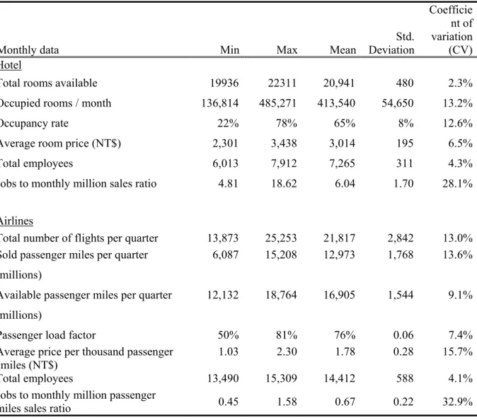
Descriptive statistics regarding the monthly operation data of tourist hotels and quarterly airline operation in Taiwan are presented in Table 1. Between 2002 and 2009, the average occupancy rate was 65% for tourist hotels with a total capacity of 20,941 rooms and 7,265
employees and managers. Hotel capacity, average room numbers, and employees remained relatively stable over these 8 years, except for the three-month period from April to June 2003, when the Taiwan tourism industry was devastated by the outbreak of the Severe Acute Respiratory Syndrome (SARS). The JSR has the biggest coefficient of variation (CV) (28%), followed by total occupied rooms (13%) and occupancy rates (12.6%). The monthly JSRs range from 4.81 to 18.62 jobs per million New Taiwan dollars (NT$) of sales.
***PLEASE INSERT TABLE 1 ABOUT HERE***
A different pattern is observed for the aviation sector. Its load factor has a much smaller coefficient of variation (7.4%), while the total number of staff employed at these two airlines remained fairly constant (between 13,490 and 15,309 during the 8-year period). The JSR, however, had a relatively large variance (CV of 32.9%). This implies that the supply of flight miles was flexible in relation to demand fluctuations so that a relatively stable load factor could be maintained. The calculated JSR is more volatile due to a stable size of the workforce and a large variation in the average price per passenger mile (P).
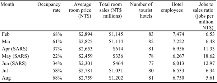
The dataset includes operational information during the SARS outbreak, which provides us with an excellent opportunity to observe the changing monthly employment structure during an extreme downtime in tourism demand. The SARS outbreak in Taiwan started in mid-April 2003 and ended on the 5th of July of that year, when Taiwan was officially removed from the World Health Organization’s list of SARS transmission areas (World Health Organization, 2003). The outbreak of the disease resulted in 674 medical cases and 84 deaths in Taiwan. The tourism industry faced dramatic reductions in the volumes of both inbound tourism and domestic tourism. Occupancy rates at tourist hotels decreased from 61% in March 2003 to 37%, 22% and 34% in the three months that followed (Table 2). In
number of hotel employees declined from 7,474 in February 2003 to 6,013 in June, representing a 19% reduction rate. We find that there was a lag of one month before the hotel industry responded to lower occupancy rates by laying-off employees: the data indicate that occupancy had hit the bottom in May, but employee numbers did not reach their lowest figures unitl June. The dramatic reduction in hotel sales and the delayed adjustment in the employment structure led to a much larger JSR when capacity utilization was extremely low (see Table 2).
***PLEASE INSERT TABLE 2 ABOUT HERE***
A similar pattern is also observed for the aviation sector, as the load factor is reduced from 72% in the first quarter of 2003 to only 50% in the second quarter. This led to the largest JSR in the 8-year time period that we consider. At the same time, the total number of flights was reduced by 25% in response to the dramatic customer reduction. The recovery of demand for flights, however, was very strong and the load factor bounced back to 80% after the SARS outbreak was declared to be over. Although labor adjustments in response to SARS in the aviation sector were relatively minor, around 280 jobs were lost (which accounted for 2% of the overall staff numbers), the two major airlines in Taiwan kept downsizing their workforce and no new positions were created till one year after the SARS period.
4.2 Variance of the JSR and the capacity utilization rate
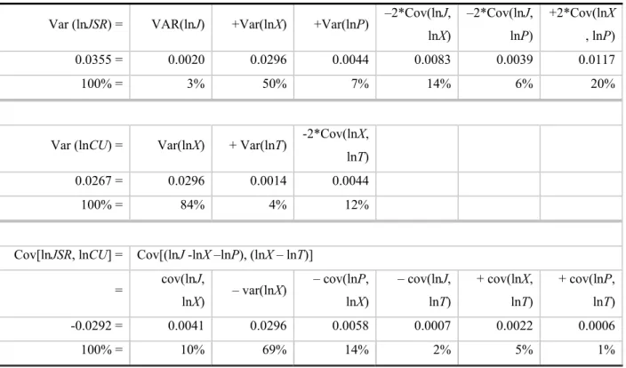
The variances of the jobs-to-sales ratio (lnJSR) and the capacity utilization rate (lnCU) can be decomposed into several components. Results are presented in Table 3. The variance of lnJSR, for example, is determined by the variances and co-variances of lnJ, lnX and lnP. The absolute values of the individual components are summed up to calculate the percentage in contribution. For the hotel sector, the component that contributes the most to the variance of
lnJSR is occupied rooms (lnX), accounting for 50% of the variation, followed by the covariance of price and occupied rooms (20%, see Table 3).
***PLEASE INSERT TABLE 3 ABOUT HERE***
The positive covariance between P and X confirms the importance of price adjustment policies in response to demand increases. Employee numbers, on the other hand, remain relatively stable without major adjustments as var(lnJ), cov(lnJ, lnX) and cov(lnJ, lnP) are very small. These results imply that a constant JSR is unlikely, because increases in jobs do not match the pace of expansion in prices and sold units.
Similarly, the covariance of lnJSR and lnCU for the hotel industry can be separated into six components. The component that contributes most to the covariance of these two variables is the number of occupied rooms (lnX, accounting for 69%), followed by the covariance of prices and occupied rooms (14%). The number of employees and the hotel capacity play a minor role in determining the covariance in lnJSR and lnCU, and there is also a weak relationship between staff numbers and numbers of occupied rooms, which again signals the rigidities of labor adjustment. This pattern provides an explanation as why most ex-ante estimates (based on a constant JSR) yield overestimations of the employment effect.
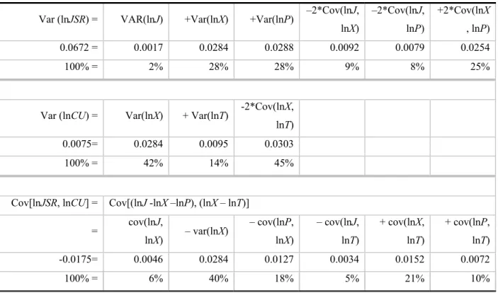
For the aviation sector, the component that contributes the most to the variance of lnJSR is average price per passenger mile (lnP) and passenger miles sold (lnX). As Table 4 shows, both factors accounted for 28% of the variation. With regard to the covariance of lnJSR and lnCU, sold passenger miles (X) and its covariance with the total capacity (T, also expressed in miles) are the two major factors. Again, the employment figure remained very stable and appears to be unrelated to sold passenger miles or total capacity. Hence, a striking similarity between the hotel and the aviation sectors is that their employee numbers do not
***PLEASE INSERT TABLE 4 ABOUT HERE***
4.3 Regression results
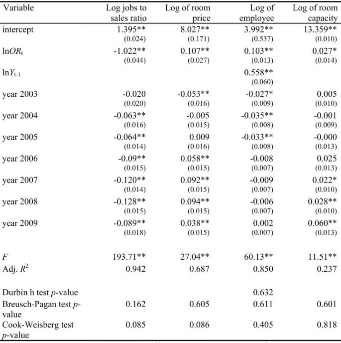
Hotel data. The lag-distributed model is applied for estimating the parameters of the equations for lnJ and lnCU, while the other three regressions are estimated using the simple linear model. The simple linear model is preferred if estimation of Equation 10 led to insignificant estimates for λ and β0. The regression results indicate that the log-transformed occupancy rates and year dummies are significant in determining the log-transformed employee numbers, room price, room capacity, and the jobs-to-sales ratio, respectively (see Table 5). Hence, we reject the null hypotheses 1 to 4 for the hotel sector. In the period we study, a 10% rise in occupancy rates led to a 10.22% decrease in the JSR, a 1.03% increase in the total staff number, a 1.07% rise in room price, and a 0.27% expansion in total room capacity.
***PLEASE INSERT TABLE 5 ABOUT HERE***
The relationship between lnJSR and lnCU is determined by lnJ, lnP, lnT and lnCU simultaneously. According to Equation 8, the effect of lnCU on the expected value of lnJSR can be computed approximately as 0.103 - 0.107 - 0.027 - 1 ≈ -1.022.6 When demand is up
6The left-hand side of Equation 8, E(lnJSR|lnCU), equals the sum of terms in the right-hand side of the
equation, E(lnJ|lnCU) – E(lnP|lnCU) – E(lnT|lnCU) – lnCU if all coefficients are estimated using the simple linear model. Because a lag-distributed model is used to estimate the expected value of lnJ conditional on lnCU, the equality of Equation 8 does not hold. Hence, the sum of βs (0.103 - 0.107 - 0.027 - 1 = -1.031) is only approximately equal to the coefficient of E(lnJSR|lnCU) (= -1.022).
and occupancy is high, per dollar of sales requires fewer numbers of employees, for several reasons. First, staff numbers do not grow at the same percentage as sales. The elasticity is only 0.103. Second, the room price appears not to be fixed. The positive correlation between room price and capacity utilization implies higher revenues per hotel room when a tourism event takes place, and consequently, fewer jobs per dollar sales. Thirdly, the overall room capacity is not constant but will fluctuate with respect to the demand level. More staff should be recruited when the house is expanding, but this does not happen to such an extent that the staff-to-room ratio remains constant. In other words, to have the assumption of a constant JSR to be valid, the increase of staff number is required to match up the adjustment of capacity utilization in the same percentage while room price and total room capacity remain unchanged during the evaluation period.
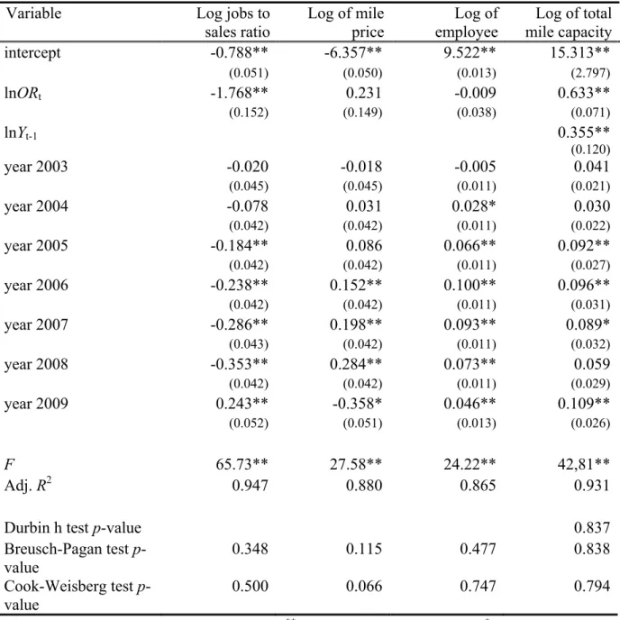
Airline data. The load factor (lnCU) significantly determines the log transformed JSR (hypothesis 4) and the log transformed total passenger capacity (hypothesis 3) at the 99% confidence level (see Table 7). The lag distributed model is applied for estimating lnCU and
lnT. The short-run propensity is 0.633, and the long-run propensity is 0.98 ( . . , which
implies that a one percent permanent increase in load factor will lead to 0.98% expansion of total flight-mile capacity over time for the aviation sector in Taiwan. Contrary to what we found for the hotel industry, prices (lnP) and total numbers of employees (lnJ) in the Taiwanese airline industry are not influenced by the load factor. The result regarding the stability of the number of employees hints at a relatively rigid human resource management in the airline industry, as airline employees on average require more specific skills, longer training period, and with fewer temporary or part time positions available than the hotel employees.
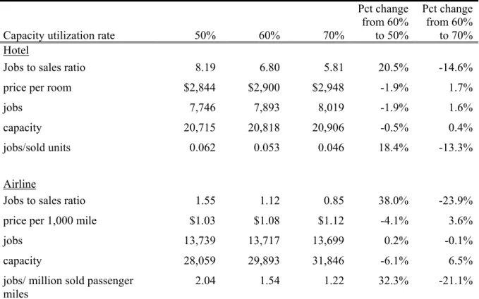
We further estimate J, P, T, and JSR for three capacity utilization levels, based on the regression results reported in Table 5 & 6. When the capacity utilization rate increases or decreases by 10% for the hotel sector, the JSR requires an adjustment of 15-20% from the baseline level (Table 7). The jobs-per-occupied-room ratio, which serves as a proxy for the labor efficiency, is also computed. This ratio decreases from 0.049 when occupancy is 60% to 0.044 when occupancy is 70%. Compared to the room price, room capacity, and the total number of employees, labor efficiency shows the largest variation. For the aviation sector, a 10% rise in load factor will lead to a 24% decrease in the JSR, compared to the 15% decrease in the hotel sector. This implies that the effects of tourism disruptions or big events on employment are likely to be overestimated to a larger extent in the airline industry than in the hotels industry, if standard input-output models are used.
***PLEASE INSERT TABLE 7 ABOUT HERE***
4.4 Simulation results for the hotel sector
To give an indication of the bias level associated with assuming a constant JSR, two scenarios are studied. In Scenario 1, we increase final demand for the lodging sector by ten million dollars. In Scenario 2, we suppose an additional occupation of a thousand rooms, as compared to baseline occupancy rates of 50%, 60% and 70%, respectively. The differences between these two scenarios are in the specification of the final demand shock (in terms of “sales value” or “sales quantity”) and the factors that are relaxed in the model.Using a fixed JSR in Scenario 1 demonstrates the error margin on direct job estimation when the adjustments of room price and labor efficiency are not considered. Scenario 2, on the other hand, allows the find demand shock to incorporate price adjustments imposed by the business
sector at different occupancies. In other words, the price factor is not assumed constant but endogenized. Thus, the error margin associated with direct job estimation using a fixed JSR only rests on the labor efficiency efficiency changes.
For Scenario 1, using the assumption of a fixed JSR, the final demand stimulus will produce 68.0 jobs, regardless of the level of occupancy (see Table 8). If we compare this with the changes implied by our regression results, the average percentage error committed by sticking to a fixed JSR is about 15-20%.
For Scenario 2, we first estimate the final demand change in dollar sales associated with the additional 1,000 rooms at 50%, 60% and 70% occupancy. This scenario resembles situations that many researchers face when carrying out impact studies of tourism, because final demand is often estimated through visitor surveys, which ask for tourists’ expenditure and shall reflect room price adjustments. When the room price increases by 1.7% as occupancy rises from 60% to 70%, the given 1,000 occupied rooms amount to final demand shocks of $2.90 million dollars, and $2.95 million dollars, respectively. Assuming a fixed JSR imposes a linear relationship between final demand changes and direct jobs estimation, thus, yielding a job figure of 19.7 at a 60% occupancy rate and 20.0 at a 70% occupancy rate. The percentage change of 1.7% simply reflects the price adjustment per room. On the contrary, the direct job effects assuming a variable JSR are 19.7 jobs and 17.1 jobs at occupancy rates of 60% and 70%, respectively. The 13% difference represents the error margin when labor efficiency is assumed constant.
***PLEASE INSERT TABLE 8 ABOUT HERE***
The results from Scenario 1 tell us that if both room price and labor efficiency are assumed constant, the biases associated to estimating direct job effects of a final demand
occupancy rate. According to our analysis regarding Scenario 2, where we relaxed the assumption of constant room prices, ceteris paribus, the bias in such job estimates is still in the range of 13% to 18%. When the assumption of constant labor efficiency is relaxed, ceteris paribus, the bias level of the job estimates is dramatically reduced to around 2%. For the case of the Taiwanese hotel sector, adjustments of labor efficiency therefore cannot be overlooked. More analyses are needed to obtain knowledge about the extent to which these results can be generalized to other tourism-related sectors, in Taiwan or elsewhere.
5. Implications for tourism impact studies
In the previous sections, we showed that using a constant JSR to predict employment effects of additional demand for tourism services would have led to overestimation in high capacity utilization situations and underestimation when demand levels are low. This pattern is observed for the Taiwanese hotel and aviation industries. We think that the level of estimation error is directly related to 1) the magnitude of demand changes, 2) the duration of the event, 3) the size of geographic region, and 4) the industry characteristics. A larger estimation error is expected for tourism applications involving dramatic demand fluctuations, within a short period for a small region. In terms of industry differences, sectors that can adjust their total service capacities, employ high-skilled personnel, and have less part-time or temporary staff would then yield larger job estimation errors. The aviation sector, the land and sea transportation sectors would fall under this category. On the other hand, the accommodation sector and the amusement sector have no flexibility in adjusting their service capacity due to physical infrastructure constraints, and most of their job positions are open for low-skilled, part time or temporary staff. For these sectors, a smaller range of variation for their jobs-to-sales ratios is expected.
To increase the accuracy of job estimates, the price effect and the labor efficiency effect should be taken into consideration simultaneously. For the price effect, some scholars have attempted to correct for the price bias by introducing the consumer price index (CPI) into the model to adjust for intertemporal price differences(Stynes et al., 2000). For short-term IO applications, this attempt only partially corrects for bias, because the short-term price change in the tourism industry is generally more substantial than suggested by the yearly CPI. For example, Porter (1999) indicated that the real room price during the 1989 and 1995 Miami Super Bowls and the 1991 Tampa Super Bowl rose by 11.26%, 19.83% and 4.44%, respectively, during the one-month period from the previous year. Practitioners therefore are recommended to take real price changes into consideration as the level of final price adjustment will be more prominent than the yearly data from the government statistics.
We also advise practitioners to include assessments of labor efficiency in the project evaluation process. Our Scenario 2 in the previous section demonstrates that changes in labor efficiency are the primary factor contributing to JSR variation. Total annual earnings, total number of persons engaged, and capacity utilization are generally made available through government statistics as most countries have routine business censuses for the manufacturing and service industries. Econometric models can be estimated using such official data.
Last, the rigidity of the recruiting system has a close link to the stages in the destination life cycle. If the region is in the exploration, involvement or development stage, infrastructures and new businesses are added to the region, and per unit sales can generally support more jobs than other stages. On the other hand, if the region has set up the lodging, dining and recreational capacity or becomes matures, additional consumption will not significantly change the numbers employed unless the opening of new business is observed. Similarly, during a tourism downtime, business entities will tend to keep their staff unless the operations of business have to be curtailed. Taiwan tourist hotels are currently situated at the
period. This is the reason why room capacity is insignificant in influencing the jobs-to-sales ratio. Since most studies focus on providing a quantitative number in economic impacts, practitioners should also collect data on the opening and closure of business entities during the evaluation period. This is where the most meaningful job creation and job losses take place.
Finally, we should stress that we only considered the direct effects of changing conditions for the tourism industry. More activity in the hotel and/or aviation sectors, for example, will also lead to increased demand for intermediate inputs in the production processes of these sectors. Up to some extent, the assumption of constant JSRs in these sectors might also be an unrealistic assumption. Furthermore, some input-output models assume that consumption levels should also be endogenized, reflecting the idea that higher income will lead to more consumption. Our study suggests that the number of new employees is not changing quickly in response to changes in tourism demand and it remains to be seen whether already employed staff members receive much more wages. If not, consumption levels will not increase very much and consequent effects of employment will not materialize.
6. Conclusion
An increasing number of economic impact studies are carried out to address special tourism demand conditions, such as hosting mega events or facing extreme weather, disease outbreaks or terrorist activities. Under these scenarios, productivity levels and cost structures of the tourism industry undergo substantial changes. Using a long-term IO model to predict the consequences of short-term events inevitably lead to estimation biases. This paper clarifies the underlying relationships between the jobs-to-sales ratio and capacity utilization.
The results indicate that the adjustment of labor efficiency is the prominent factor in determining the stability of the jobs-to-sales ratio, while price, total employee number and service capacity are relatively stable in response to demand changes. For the hotel sector, a 10% fluctuation in the occupancy rate leads to a 15-20% adjustment in the jobs-to-sales ratio, 2% in room price, 2% in employees and 13-18% in labor efficiency. For the aviation sector, a 10% fluctuation in the load factor resulted in a 24-38% adjustment in the jobs-to-sales ratio, 5% in total passenger miles offered, and 21-32% in labor efficiency. The magnitude of biases associated with assuming a stable job-to-sales ratio is too large to be ignored. While Frechtling (2006), Stynes & White (2006) and Wilton & Nickerson (2006) indicated that the possibly largest errors of tourism economic impact estimation are caused by the inaccuracy of forecasts (or measurement) of visitor numbers and average spending, we argue that stability of economic and technological ratios representing production processes in the tourism industry should also be considered with care.
The implications of this study can also be integrated into Computable General Equilibrium models (CGE), which generally assume constant returns to scale and incorporate the price mechanism to clear all markets simultaneously (Blake & Gillham, 2001; Dwyer et al., 2004). This study indicates that only taking the price adjustment mechanism into account is insufficient in reaching a satisfactory portrayal of the reality in labor usages per unit output. The adjustment of labor efficiency during various level of capacity utilization should be acknowledged and endogenized in the system to allow for changing returns to utilization so that more accurate job estimates can be provided.
Constructive comments from Dr. Bart Los at University of Groningen, and two anonymous referees are highly appreciated. Financial support from the Taiwan National Science Council under NSC98-2410-H-390-029-SS2 is acknowledged.
7. References
Ahlert, G. (2001). The Economic Effects of the Soccer World Cup 2006 in Germany with Regard to Different Financing. Economic Systems Research, 13, 109 - 127.
Archer, B. (1977). Tourism multipliers: The state of art. Cardiff: University of Wales Press. Arenberg, Y. (1991). Service capacity, demand fluctuations, and economic behavior.
American Economist, 35, 52-55.
Baade, R. A., & Matheson, V. A. (2003). Bidding for the Olympics: Fool's gold? In C. Barros, M. Ibrahim & S. Szymanski (Eds.), Transatlantic Sport (pp. 127-151). London: Edward Elgar Publishing.
Baade, R. A., & Matheson, V. A. (2004). The quest for the cup: Assessing the economic impact of the World Cup. Regional Studies, 38, 343-354.
Baade, R. A., & Matheson, V. A. (2006). Padding required: Assessing the economic impact of the super bowl. European Sports Management Quarterly, 6, 353-374.
Baltagi, B. H., Griffin, J. M., & Vadali, S. R. (1998). Excess capacity: A permanent characteristic of US airlines? Journal of Applied Econometrics, 13, 645-757.
Berndt, E. R., & Morrison, C. J. (1981). Capacity utilization measures: Underlying economic theory and an alternative approach. American Economic Review, 71, 48-52.
Blake, A., & Gillham, J. (2001). A Multi-Regional CGE Model of Tourism in Spain. Paper presented at the European Trade Study Group annual conference, Brussels.
Blake, A., & Sinclair, M. T. (2003). Tourism crisis management: US Response to September 11. Annals of Tourism Research, 30, 813-832.
Blake, A., Sinclair, M. T., & Sugiyarto, G. (2003). Quantifying the impact of foot and mouth disease on tourism and the UK economy Tourism Economics, 9, 449-465.
Borooah, V. K. (1999). The supply of hotel rooms in Queensland, Australia. Annals of Tourism Research, 26, 985-1003.
Bryden, J. M. (1973). Tourism and development: A case study of the Commonwealth Caribbean. Cambridge, England: University Press.
Caves, D. W., & Christensen, L. R. (1988). The importance of economies of scale, capacity utilization, and density in explaining interindustry differences in productivity growth. Logistics and Transportation Review, 24, 3-32.
Coates, D., & Humphreys, B. R. (2003). Professional sports facilities, franchises and urban economic development. Public Finance and Management, 3, 335-357.
Conway, R. S. (1980). Changes in regional Input-Output coefficients and regional forecasting. Regional Science and Urban Economics, 10, 153-171.
Crompton, J. L. (1995). Economic impact analysis of sports facilities and events: Eleven sources of misapplication. Journal of Sport Management, 9, 14-35.
Dwyer, L., Forsyth, P., Spurr, R., & Ho, T. (2004). The economic impacts and benefits of tourism in Australia: A general equilibrium approach. In C. Cooper (Ed.). Southport, AU: Cooperative Research Centre for Sustainable Tourism.
Fletcher, J., & Snee, H. (1989). Tourism multiplier effects. In S. F. Witt & L. Moutinho (Eds.), Tourism Marketing and Management Handbook (pp. 529-531). Hertfordshire, UK: Prentice Hall International Ltd. (UK).
Forssell, O. (1972). Explaining changes in input-output coefficients for Finland. In A. Brody & A. P. Carter (Eds.), Input-Output Techniques (pp. 343-369). Amsterdam:
North-Frechtling, D. C. (2006). An assessment of visitor expenditure methods and models. Journal of Travel Research, 45, 26-35.
Gasparino, U., Bellini, E., Corpo, B. D., & Malizia, W. (2008). Measuring the impact of tourism upon urban economies: A review of literature FEEM working paper series. Milan: The Fondazione Eni Enrico Mattei.
Gujarati, D. N., & Porter, D. C. (2009). Basic Econometrics (5th ed.). New York: The McGraw-Hill companies, Inc.
Hagn, F., & Maenning, W. (2009). Large sport events and unemployment: The case of the 2006 soccer World Cup in Germany. Applied Economics, 41, 3295-3302.
Hatch, J. H. (1986). The impact of the Grand Prix on the restaurant industry. In J. P. A. Burns, J. H. Hatch & T. J. Mules (Eds.), The Adelaide Grand Prix - The impact of a special event: The Centre for South Australian Economic Studies.
Krakover, S. (2000). Partitioning seasonal employment in the hospitality industry. Tourism Management, 21, 461-471.
Lee, C.-K., & Taylor, T. (2005). Critical reflections on the economic impact assessment of a mega-event: the case of 2002 FIFA World Cup. Tourism Management, 26, 595-603. Miller, R. E., & Blair, P. D. (1985). Input-output analysis: Foundations and extensions.
Englewood Cliffs, N.J.: Prentice-Hall.
Porter, P. K. (1999). Mega-sports events as municipal investments: A critique of impact analysis. In J. Fizel, E. Gustafson & L. Hadley (Eds.), Sports Economics: Current Research (pp. 61-74). Westport, Connecticut: Praeger Publishers.
Porter, P. K., & Fletcher, D. (2008). The economic impact of the Olympic Games: Ex ante predictions and ex poste reality. Journal of Sport Management, 22, 470-486.
Price Water House Coopers. (2005). Olympic Games Impact Study. London: Price Water House Coopers LLP.
Rose, A., & Miernyk, W. (1989). Input-output analysis: The first fifty years. Economic Systems Research, 1, 229-271.
Stynes, D. J., Propst, D. B., Chang, W., & Sun, Y. (2000). Estimating national park visitor spending and economic impacts: The MGM2 model. Final report to National Park Service. East Lansing, Michigan: Department of Park, Recreation and Tourism Resources, Michigan State University.
Stynes, D. J., & White, E. M. (2006). Reflections on measuring recreation and travel spending. Journal of Travel Research, 45, 8-16.
Sun, Y.-Y. (2007). Adjusting Input-Output models for capacity utilization in service industries. Tourism Management, 28, 1507-1517.
Szymanski, S. (2002). The economic impact of the World Cup. World Economics, 3, 169-177.
Taiwan Stock Exchange Cooperation. (2009). Market Observation Post System (MOPS), from http://emops.tse.com.tw/emops_all.htm
Taiwan Tourism Bureau. (2002-2009). The operating report of international tourist hotels in Taiwan. Taipei, Taiwan: Tourism Bureau, Ministry of Transportation and Communications, R.O.C.
Toohey, K., & Veal, A. J. (2007). The Olympic Games: A social science perspective (2nd ed.). Oxfordshire, UK: CABI International.
Vaccara, B. N. (1971). An Input-Output model for long-range economic projections. Survey of Current Business, 51, 47-56.
West, G. (1995). Comparison of Input-Output, Input-Output Econometric and Computable General Equilibrium Impact Models at the regional level. Economic Systems Research, 7, 209-227.
Wilton, J. J., & Nickerson, N. P. (2006). Collecting and using visitor spending data. Journal of Travel Research, 45, 17-25.
Wooldridge, J. M. (2009). Introductory Econometrics: A Modern Approach (4th ed.). Cincinnati, OH: South-Western.
World Health Organization. (2003). Taiwan, China: SARS transmission interrupted in last outbreak area Retrieved June 16, 2007,
from http://www.who.int/csr/don/2003_07_05/en/
Yang, H.-Y., & Chen, K.-H. (2009). A general equilibrium analysis of the economic impact of a tourism crisis: A case study of the SARS epidemic in Taiwan. Journal of Policy Research in Tourism, Leisure and Events, 1, 37-60.
Table 1. Descriptive statistics of monthly tourist hotel operations and quarterly airline operation in Taiwan (2002-2009)
Monthly data Min Max Mean
Std. Deviation Coefficie nt of variation (CV) Hotel
Total rooms available 19936 22311 20,941 480 2.3% Occupied rooms / month 136,814 485,271 413,540 54,650 13.2%
Occupancy rate 22% 78% 65% 8% 12.6%
Average room price (NT$) 2,301 3,438 3,014 195 6.5% Total employees 6,013 7,912 7,265 311 4.3% Jobs to monthly million sales ratio 4.81 18.62 6.04 1.70 28.1%
Airlines
Total number of flights per quarter 13,873 25,253 21,817 2,842 13.0% Sold passenger miles per quarter
(millions)
6,087 15,208 12,973 1,768 13.6%
Available passenger miles per quarter (millions)
12,132 18,764 16,905 1,544 9.1%
Passenger load factor 50% 81% 76% 0.06 7.4% Average price per thousand passenger
miles (NT$)
1.03 2.30 1.78 0.28 15.7% Total employees 13,490 15,309 14,412 588 4.1% Jobs to monthly million passenger
Table 2. Statistics on tourist hotels before, during, and after the SARS period, 2003 Month Occupancy rate Average room price (NT$) Total room sales (NT$ millions) Number of tourist hotels Hotel employees Jobs to sales ratio (jobs per million NT$) Feb 68% $2,894 $1,145 83 7,474 6.53 Mar 61% $2,825 $1,114 82 7,222 6.48 Apr (SARS) 37% $2,653 $614 81 6,956 11.33 May (SARS) 22% $2,459 $336 78 6,267 18.62 Jun (SARS) 34% $2,301 $464 77 6,013 12.97 Jul 58% $2,781 $1,031 80 6,533 6.34 Aug 68% $2,759 $1,202 81 6,750 5.61
Table 3. Variance components analysis of lnJSR and lnCU for the hotel sector
Var (lnJSR) = VAR(lnJ) +Var(lnX) +Var(lnP) –2*Cov(lnJ,
lnX) –2*Cov(lnJ, lnP) +2*Cov(lnX , lnP) 0.0355 = 0.0020 0.0296 0.0044 0.0083 0.0039 0.0117 100% = 3% 50% 7% 14% 6% 20%
Var (lnCU) = Var(lnX) + Var(lnT) -2*Cov(lnX,
lnT)
0.0267 = 0.0296 0.0014 0.0044
100% = 84% 4% 12%
Cov[lnJSR, lnCU] = Cov[(lnJ -lnX –lnP), (lnX – lnT)]
= cov(lnJ, lnX) – var(lnX) – cov(lnP, lnX) – cov(lnJ, lnT) + cov(lnX, lnT) + cov(lnP, lnT) -0.0292 = 0.0041 0.0296 0.0058 0.0007 0.0022 0.0006 100% = 10% 69% 14% 2% 5% 1%
Table 4. Variance components analysis of lnJSR and lnCU for the airline sector
Var (lnJSR) = VAR(lnJ) +Var(lnX) +Var(lnP) –2*Cov(lnJ,
lnX) –2*Cov(lnJ, lnP) +2*Cov(lnX , lnP) 0.0672 = 0.0017 0.0284 0.0288 0.0092 0.0079 0.0254 100% = 2% 28% 28% 9% 8% 25%
Var (lnCU) = Var(lnX) + Var(lnT) -2*Cov(lnX,
lnT) 0.0075= 0.0284 0.0095 0.0303
100% = 42% 14% 45%
Cov[lnJSR, lnCU] = Cov[(lnJ -lnX –lnP), (lnX – lnT)]
= cov(lnJ, lnX) – var(lnX) – cov(lnP, lnX) – cov(lnJ, lnT) + cov(lnX, lnT) + cov(lnP, lnT) -0.0175= 0.0046 0.0284 0.0127 0.0034 0.0152 0.0072 100% = 6% 40% 18% 5% 21% 10%
Table 5. Regression results for the hotel data, 2002-2009
Variable Log jobs to
sales ratio Log of room price employee Log of Log of room capacity intercept 1.395** (0.024) 8.027** (0.171) 3.992** (0.537) 13.359** (0.010) lnORt -1.022** (0.044) 0.107**(0.027) 0.103** (0.013) 0.027*(0.014) lnYt-1 0.558** (0.060) year 2003 -0.020 (0.020) -0.053** (0.016) -0.027* (0.009) 0.005 (0.010) year 2004 -0.063** (0.016) -0.005 (0.015) -0.035** (0.008) -0.001 (0.009) year 2005 -0.064** (0.014) 0.009 (0.016) -0.033** (0.008) -0.000 (0.013) year 2006 -0.09** (0.015) 0.058**(0.015) -0.008 (0.007) (0.013)0.025 year 2007 -0.120** (0.014) 0.092**(0.015) -0.009 (0.007) 0.022*(0.010) year 2008 -0.128** (0.015) 0.094** (0.015) -0.006 (0.007) 0.028** (0.010) year 2009 -0.089** (0.018) 0.038** (0.015) 0.002 (0.007) 0.060** (0.013) F 193.71** 27.04** 60.13** 11.51** Adj. R2 0.942 0.687 0.850 0.237
Durbin h test p-value 0.632 Breusch-Pagan test
p-value 0.162 0.605 0.611 0.601
Cook-Weisberg test p-value
0.085 0.086 0.405 0.818
Standard error statistics are in parentheses.**Significant at the 99% level; *significant at the 95% level.
Table 6. Regression results for the airline data, 2002-2009
Variable Log jobs to
sales ratio Log of mile price employee Log of mile capacityLog of total
intercept -0.788** -6.357** 9.522** 15.313** (0.051) (0.050) (0.013) (2.797) lnORt -1.768** 0.231 -0.009 0.633** (0.152) (0.149) (0.038) (0.071) lnYt-1 0.355** (0.120) year 2003 -0.020 -0.018 -0.005 0.041 (0.045) (0.045) (0.011) (0.021) year 2004 -0.078 0.031 0.028* 0.030 (0.042) (0.042) (0.011) (0.022) year 2005 -0.184** 0.086 0.066** 0.092** (0.042) (0.042) (0.011) (0.027) year 2006 -0.238** 0.152** 0.100** 0.096** (0.042) (0.042) (0.011) (0.031) year 2007 -0.286** 0.198** 0.093** 0.089* (0.043) (0.042) (0.011) (0.032) year 2008 -0.353** 0.284** 0.073** 0.059 (0.042) (0.042) (0.011) (0.029) year 2009 0.243** -0.358* 0.046** 0.109** (0.052) (0.051) (0.013) (0.026) F 65.73** 27.58** 24.22** 42,81** Adj. R2 0.947 0.880 0.865 0.931
Durbin h test p-value 0.837
Breusch-Pagan test
p-value 0.348 0.115 0.477 0.838
Cook-Weisberg test p-value
0.500 0.066 0.747 0.794
Standard error statistics are in parentheses. **Significant at the 99% level; *significant at the 95% level.
Table 7. Predicted results based on different capacity utilization rates
Capacity utilization rate 50% 60% 70%
Pct change from 60% to 50% Pct change from 60% to 70% Hotel
Jobs to sales ratio 8.19 6.80 5.81 20.5% -14.6% price per room $2,844 $2,900 $2,948 -1.9% 1.7%
jobs 7,746 7,893 8,019 -1.9% 1.6%
capacity 20,715 20,818 20,906 -0.5% 0.4% jobs/sold units 0.062 0.053 0.046 18.4% -13.3%
Airline
Jobs to sales ratio 1.55 1.12 0.85 38.0% -23.9% price per 1,000 mile $1.03 $1.08 $1.12 -4.1% 3.6%
jobs 13,739 13,717 13,699 0.2% -0.1%
capacity 28,059 29,893 31,846 -6.1% 6.5% jobs/ million sold passenger
miles
2.04 1.54 1.22 32.3% -21.1% Note: The J/X ratio is computed by dividing the predicted jobs by the predicted occupied rooms at the given occupancy rate.
Table 8. Estimation results based on two scenarios
Occupancy rate 50% 60% 70% Pct change from 60% to 50% Pct change from 60% to 70% Scenario 1: Ten million dollars of final demand changes
direct jobs - fixed ratio1 68.0 68.0 68.0 0.0% 0.0% direct jobs - predicted ratio2 81.9 68.0 58.1 20.5% -14.6% Scenario 2: Per 1,000 occupied rooms
Room sales (millions) $2.84 $2.90 $2.95 -1.9% 1.7% direct jobs - fixed ratio1 19.3 19.7 20.0 -1.9% 1.7% direct jobs - predicted ratio2 23.3 19.7 17.1 18.1% -13.2% 1 Standard IO analysis assumes a fixed jobs to sales ratio.