利用隨機配置陣列發展遠場聲學影像演算法

國 立 交 通 大 學

機械工程學系

碩士論文

利用隨機配置陣列發展遠場聲學影像演算法

Development of far-field acoustic imaging algorithms

using an optimized random array

研 究 生: 劉冠良

指導教授: 白明憲

利用隨機配置陣列發展遠場聲學影像演算法

Development of far-field acoustic imaging algorithms

using an optimized random array

研 究 生：劉冠良

Student：Kuan-Liang Liu

指導教授：白明憲

Advisor：Mingsian R. Bai

國 立 交 通 大 學

機械工程學系

碩 士 論 文

A thesis

Submitted to Department of Mechanical Engineering

Collage of Engineering

National Chiao Tung University

In Partial Fulfillment of Requirements

for the Degree of Master of Science

in

Mechanical Engineering

June 2009

HsinChu, Taiwan, Republic of China

利用隨機配置陣列發展遠場聲學影像演算法

研究生：劉冠良 指導教授：白明憲 教授

國立交通大學機械工程學系

摘 要

稀疏且隨機配置的麥克風陣列已知可以用來傳遞遠場的影像而

不會產生鬼葉瓣的問題。在這篇論文中，數值模擬被用來最佳化麥克

風的配置。全域最佳化技術包括蒙地卡羅法、模擬退火法和內部方格

蒙地卡羅法被用來有效率地尋找最佳的麥克風配置。如常理所知，模

擬結果顯示出要避免鬼葉瓣的出現，隨機配置麥克風是必要的。而結

合模擬退火法和蒙地卡羅法的方法可以有效率的找到一個令人滿意

的配置，這個配置能得到傑出的波束圖和相對較均勻的麥克風分布。

在到達方向的估測中，平面波的聲源被視為球面波。遠場聲學影像的

方法包括延遲和相加法、時間反轉法、單進多出等效聲源反逆濾波

法、最小變異無失真響應法和多重信號分類法被用來估測聲源位置。

結果顯示多重信號分類法在定位噪音源位置上可得到最佳的結果。

Far-field microphone array systems

Student: Kuan-Liang Liu Advisor: Mingsian R. Bai

Department of Mechanical Engineering National Chiao-Tung University

A

BSTRACT

Arrays with sparse and random microphone deployment are known to be capable of delivering high quality far-field images without grating lobes. Numerical simulations are undertaken in this thesis to optimize the microphone deployment. Global optimization techniques including the Monte Carlo (MC) algorithm, the Simulated Annealing (SA) algorithm and the Intra-Block Monte Carlo (IBMC) algorithms are exploited to find the optimal microphone deployment efficiently. As predicted by the conventional wisdom, the results reveal that randomized deployment is required to avoid grating lobes. The combined use of the SA and the IBMC algorithms enables efficient search for satisfactory deployment with excellent beam pattern and relatively uniform distribution of microphones. In Direction of arrival (DOA) estimation, the planar wave sources are assumed to be spherical wave sources in this thesis. Far-field acoustic imaging algorithms including the delay and sum (DAS) algorithm, the time reversal (TR) algorithm, the single input multiple output equivalent source inverse filtering (SIMO-ESIF) algorithm, the Minimum Variance Distortionless Response (MVDR) algorithm and the Multiple Signal Classification (MUSIC) algorithm are employed to estimate DOA. Results show that the MUSIC

algorithm can attain the highest resolution of localizing sound sources positions.

誌謝

時光飛逝，短短兩年的研究生生涯轉眼將成往事。首先要感謝指導教授白明 憲博士的諄諄教誨。在兩年的時間裡，深刻的感受到教授追求學問的熱忱與執 著，也很佩服教授淵博的學問與遇到問題會積極解決的研究態度。在教授豐富的 專業知識以及嚴謹的治學態度下，使我能夠順利完成學業與論文，在此致上最誠 摯的謝意。 在論文寫作方面，感謝本系成維華教授和呂宗熙教授在百忙中撥冗閱讀，並 提出寶貴的意見與指導，使得本文的內容更趨完善與充實，在此致上無限的感激。 回顧兩年來的日子，承蒙同實驗室的博士班陳榮亮學長、林家鴻學長、李雨 容學姐，以及碩士班洪志仁學長、謝秉儒學長在研究與學業上的適時指點，並有 幸與王俊仁同學、郭育志同學、何克男同學、艾學安同學互相切磋討論，讓我獲 益甚多。此外學弟妹曾智文、廖國志、張濬閣、陳俊宏、廖士涵、桂振益、劉孆 婷在生活上的朝夕相處與砥礪磨練，亦值得細細回憶。因為有了你們，讓實驗室 裡總是充滿歡笑，也讓這兩年的光陰更增添回憶。 最後僅以此篇論文，獻給我摯愛的家人，雙親劉昌雄先生、周素美女士、姑 姑劉梨雪小姐、兩位弟弟劉彥良及劉長霖，這一路上，因為有你們的付出與支持， 給了我最大的精神支柱，也讓我有勇氣面對更艱難的挑戰。要感謝的人很多，上 述名單恐有疏漏，在此一併致上我由衷的謝意。

T

ABLE OF

C

ONTENTS

摘 要 ... I 

ABSTRACT ... II  誌謝 ... IV 

TABLE OF CONTENTS ... V 

LIST OF TABLES ... VII 

LIST OF FIGURES ... VIII 

Introduction ... 1 

1.  Beam pattern and cost function ... 4 

2.  Optimization algorithms ... 5 

2.1  Intra-Block Monte Carlo (IBMC) simulation ... 5 

2.2  Simulated Annealing (SA) technique ... 6 

2.3  Numerical simulations for optimization algorithms ... 8 

2.3.1  Optimizing array deployment without IB constraint ... 8 

2.3.2  Optimizing array deployment with IB constraint ... 10 

3.  Methods for Direction of Arrival (DOA) estimation ... 13 

3.1  DAS algorithm ... 13 

3.2  TR algorithm ... 15 

3.3  SIMO-ESIF algorithm ... 15 

3.4  Minimum Variance Distortionless Response (MVDR)algorithm ... 17 

3.5  Multiple Signal Classification (MUSIC) algorithm ... 19 

3.6  Numerical simulations of DOA algorithms ... 22 

4. Experimental verifications ... 25 

4.1  Loudspeakers experiment ... 26 

4.2  Compressor experiment ... 26 

5. Conclusion ... 28  REFERENCES ... 29 

L

IST OF

T

ABLES

Table 1. The search performance of different optimization methods for array deployment with the inter-element spacing d = 0.6 m (3λ at the frequency 1.7 kHz). The letter “w” indicates that weight optimization is performed. ... 32  Table 2. The comparison of converged cost function Q of the URA and the optimized

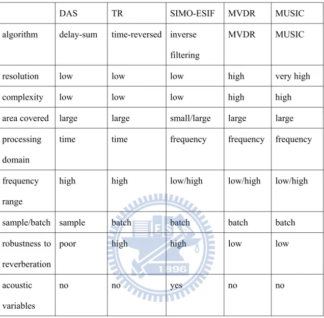
random arrays at three different frequencies. ... 33  Table 3. Lagrange interpolation FIR filter coefficients for N = 1 and N = 2 ... 34  Table 4. Comparisons of acoustic imaging algorithms. ... 35 

L

IST OF

F

IGURES

Fig 1. A plane wave incident from the direction κ to a far-field array. ... 36  Fig 2. The schematic diagram of localized regions and grid points. (a) The

localized regions (dashed lines) on the microphone surface with the inter-element spacing d = 0.6m. The symbol “ □ ＂ indicates the microphone position. (b) The grid on a localized region. The microphone is constrained to move to one of nine grid points (including itself) in the far-field optimization. The microphone is assigned to any grid point in the localized region in the near-field optimization for the SA search. ... 37  Fig 3. The flowchart of the IBMC optimization algorithm. ... 38  Fig 4. The flowchart of the SA optimization algorithm. ... 39  Fig 5. The URA with inter-element spacing 0.6m (3λ at the frequency 1.7 kHz). (a) Array deployment, (b) beam pattern. ... 40  Fig 6. The array optimized using the MC algorithm without the IB constraint at the

frequency 1.7 kHz. Maximum cost function Q = 2.6532 is attained at the 27596th iteration. The circle indicates the main-lobe. (a) Learning curve, (b) optimal array deployment, (c) beam pattern. ... 42  Fig 7. The array optimized using the SA algorithm without the IB constraint at the

frequency 1.7 kHz. Maximum cost function Q = 2.7561 is attained at the 1283rd iteration. The circle indicates the main-lobe. (a) Learning curve, (b) optimal array deployment, (c) beam pattern with deployment optimized, (d) beam pattern with weights optimized. ... 44  Fig 8. The array optimized using the IBMC algorithm at the frequency 1.7 kHz.

Maximum cost function Q = 2.5638 is attained at the 7662nd iteration. The circle indicates the main-lobe. (a) Learning curve, (b) optimal array deployment, (c) beam pattern. ... 46 

Fig 9. The array optimized using the combined SA-IBMC algorithm with the IB constraint at the frequency 1.7 kHz. Maximum cost function Q = 2.6602 is attained at the 1429th iteration. The circle indicates the main-lobe. (a) Learning curve, (b) optimal array deployment obtained by SA, (c) beam pattern obtained by SA, (d) optimal array deployment obtained by SA-IBMC search, (e) beam pattern obtained by SA-IBMC, (f) beam pattern with

weights optimized. ... 49 

Fig 10. A uniform rectangular array (URA). A point sound source is located at far-field. ... 50 

Fig 11. The DAS beamformer. ... 51 

Fig 12. The block diagram of the TR algorithm. ... 52 

Fig 13. The block diagram of the SIMO-ESIF algorithm. ... 53 

Fig 14. Decide source numbers by AIC algorithm. The truncated order is corresponded to the lowest point. (a) Error, weight and AIC lines, (b) AIC lines with different weights. ... 54 

Fig 15. The array configurations for DOA estimation simulations and experiments. (a) URA and (b) optimized random array. ... 55  Fig 16. The noise maps of two simulated point sources obtained using five acoustic

imaging algorithms with 30-channel URA and random array. The squares are the preset sound source positions. The simulated whitenoise sources located at the positions (-0.5m, 0.5m) and (0.5m, -0.5m). The observed frequency is 1 kHz (d =λ/ 4). The power spectrums obtained using (a) DAS with URA configuration, (b) DAS with random array configuration, (c) TR with URA configuration, (d) TR with random array configuration, (e) SIMO-ESIF with URA configuration, (f) SIMO-ESIF with random array configuration, (g) MVDR with URA configuration, (h) MVDR with random

array configuration, (i) MUSIC with URA configuration and (j) MUSIC with random array configuration. ... 61  Fig 17. The noise maps of two simulated point sources obtained using five acoustic

imaging algorithms with 30-channel URA and random array. The squares are the preset sound source positions. The simulated whitenoise sources located at the positions (-0.5m, 0.5m) and (0.5m, -0.5m). The observed frequency is 7 kHz (d =2λ). The power spectrums obtained using (a) DAS with URA configuration, (b) DAS with random array configuration, (c) TR with URA configuration, (d) TR with random array configuration, (e) SIMO-ESIF with URA configuration, (f) SIMO-ESIF with random array configuration, (g) MVDR with URA configuration, (h) MVDR with random array configuration, (i) MUSIC with URA configuration and (j) MUSIC with random array configuration. ... 67  Fig 18. Beamformer properties at 30o opening angle. ... 68  Fig 19. The experimental arrangement for loudspeakers measurements inside a

semi-anechoic chamber. An optimized random array is used to deploy 30 microphones. ... 69  Fig 20. The noise maps of two loudspeakers obtained using five acoustic imaging

algorithms with 30-channel URA and random array. The squares are the preset sound source positions. The simulated whitenoise sources located at the positions (-0.5m, 0.5m) and (0.5m, -0.5m). The observed frequency is 1 kHz (d =λ/ 4). The power spectrums obtained using (a) DAS with URA configuration, (b) DAS with random array configuration, (c) TR with URA configuration, (d) TR with random array configuration, (e) SIMO-ESIF with URA configuration, (f) SIMO-ESIF with random array configuration, (g) MVDR with URA configuration, (h) MVDR with random array

configuration, (i) MUSIC with URA configuration and (j) MUSIC with random array configuration. ... 74  Fig 21. The noise maps of two loudspeakers obtained using five acoustic imaging

algorithms with 30-channel URA and random array. The squares are the preset sound source positions. The simulated whitenoise sources located at the positions (-0.5m, 0.5m) and (0.5m, -0.5m). The observed frequency is 7 kHz (d =2λ). The power spectrums obtained using (a) DAS with URA configuration, (b) DAS with random array configuration, (c) TR with URA configuration, (d) TR with random array configuration, (e) SIMO-ESIF with URA configuration, (f) SIMO-ESIF with random array configuration, (g) MVDR with URA configuration, (h) MVDR with random array configuration, (i) MUSIC with URA configuration and (j) MUSIC with random array configuration. ... 80  Fig 22. Noise map of a compressor obtained using MUSIC method. The observed

frequency is 1 kHz. ... 82  Fig 23. Noise map of a scooter obtained using MUSIC method. The observed

Introduction

Array technology has been used in many diverse areas including radar [1], sonar [2], radio astronomy [3], tele-communications [4], and so forth. Its application encompasses purposes including signal enhancement, spatial filtering, Direction of Arrival (DOA) estimation, etc. Early development of arrays or beamformers was primarily based on the far-field assumption that the source is far away and the waves become planar at the array position. Far-field arrays are particularly useful for long distance and large scale sources such as wind tunnels [5], trains and aircrafts. In array implementation, transducer deployment has been one of the key issues. It is well known that, for uniform linear arrays (ULA) and uniform rectangular arrays (URA) [6], array deployment must comply with the λ/2-rule to avoid the spatial aliasing and the grating lobe problems [7]. Consequently, a large number of microphones are required to cover the source area, which can render the array configuration impractical for sources at high frequencies. This prompts the development of non-uniform arrays that are capable of achieving high resolution and aliasing-free imaging with sparse sensors [8]. Knowing the fact that non-uniform spacing can be beneficial to far-field array performance, however, a question arises naturally. What is the optimal deployment of far-field random arrays? To explore this conjecture, numerical simulation is undertaken in this thesis with the aid of optimization techniques.

Several global optimization techniques are employed to deploy microphones for planar arrays used in far-field imaging. Monte Carlo (MC) simulation [9-13] is based on straightforward random search. Despite its simplicity, the MC method can be very time consuming. A more efficient technique, the simulated annealing (SA) algorithm [8, 14-16] is also used in the simulation. The SA algorithmrelies on a search principle resembling the annealing process in the metallurgy. The search

process follows an annealing schedule dictated by a temperature-dependent probability. The probability of accepting “worse” solutions in the initial high-temperature stage lends the SA method an effective approach for problems with many local minima [15]. Several researchers have applied the SA algorithm to optimize far-field arrays [17, 18]. In this these, modifications are made to enhance the search for optimal deployment. The Intra-Block Monte Carlo (IBMC) method conducts the random search only in the pre-partitioned local regions. This approach enhances search efficiency and often results in relatively uniform sensor deployment. A hybrid approach combining the SA and the IBMC methods is also presented to improve the search performance. The simulation results obtained using the MC, SA and SA-IBMC approaches, with and without IB constraint, are compared in terms of number of iterations and the maximum cost function values in Table 1.

In DOA estimation, the random array optimized by SA-IBMC method is used. There are several far-field acoustic imaging algorithms have been proposed in the past. For low resolution algorithms, the delay and sum (DAS) beamformer applies time shifts to the array signals to compensate for the propagation delays in the arrival of the source signal at each microphone [19-20]. The single input multiple output equivalent source inverse filtering (SIMO-ESIF) method is a technique based on designing inverse filters to minimize the error between the estimate sources and the original sources [21]. For high resolution algorithms, the Minimum Variance Distortionless Response (MVDR) algorithm adaptively finds weights to improve source resolution that minimizes the output noise variance due to signals that arrive from directions other than hypothesized source direction [19, 22-24]. The idea of Multiple Signal Classification (MUSIC) algorithm is that the eigenvalues and eigenvectors of a signal covariance matrix are used to estimate the DOA of multiple signals received by a sensor array [19, 25, 26]. In addition to planar wave sources,

spherical wave sources have been assumed for source resolution [20, 26-27]. The simulated and experimental results of these algorithms are examined in resolution and summarized in a compared table.

1. Beam pattern and cost function

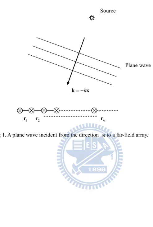
For a far-field array, the beam pattern can be defined in the wave number domain [20] 1 1 M m m j b M =

e

=

∑

k ri , (1) where k=ω/c is the wave number, ω is angular frequency, c is the speed of

sound, and r_m is the position vector of the mth microphone, k= −kκ is the wave number vector of a plane wave incident from the direction represented by the unit vector κ and M is number of microphone, as shown in Fig. 1.

In optimizing far-field performance, the aim is to minimize the maximum side-lobe level (MSL) of the beam pattern [20]. First, a circle with radius is drawn on the kx-ky plane to define the scope of the main-lobe, which is a judicious

choice based on the beam pattern observations. The exterior of this circle is considered the side-lobe region. The cost function for far-field arrays is defined as

m r m Q s = , (2)

where and denote the maxima of the main-lobe and the side-lobes, respectively. Because m = 1, the cost function amounts to minimize the MSL and maximizing .

m s

2. Optimization algorithms

In this section, global optimization methods for microphone deployment are presented.

2.1 Intra-Block Monte Carlo (IBMC) simulation

The basic MC algorithm is based on straightforward random search. It often tends to be used when it is unfeasible or impossible to compute an exact result with a deterministic algorithm [9]. For M microphones to be allocated to

rectangular grid points, the number of possible combinations is , which is known to be an NP-complete problem [28]. Due to the blind search nature, the MC algorithm can be very inefficient and result in non-uniform distribution of microphones that concentrate at certain areas. To address these problems, a modified method IBMC is proposed.

(m+ × +1) (n 1 (m+ × +1) (n 1) ) d M C

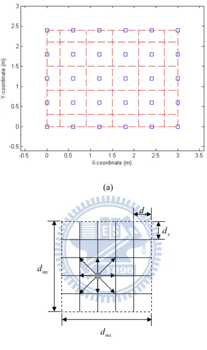
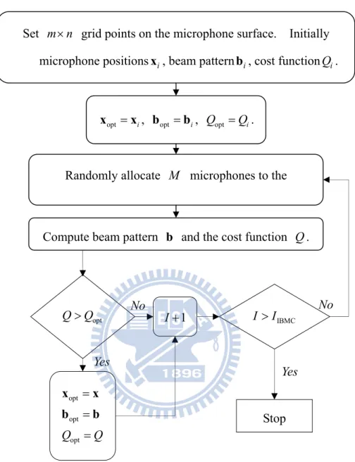
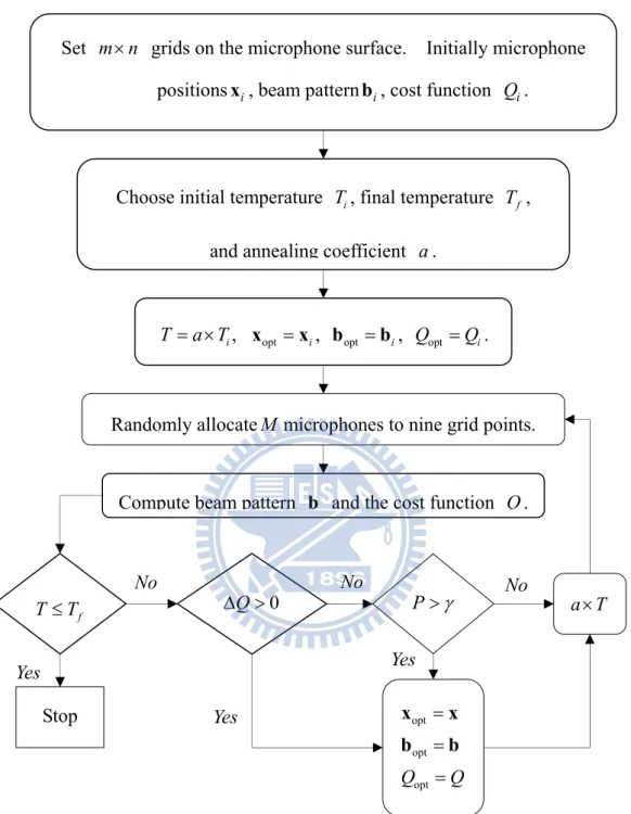
By “Intra-Block”, we mean the localized region designated to each microphone on the surface, as shown in Fig. 2 (a). The MC search is only conducted within each block with random positions generated inside this designated region. The M

microphone elements will be designated to M localized regions. Hence, each region

necessarily contains one and only one microphone. The flowchart of IBMC is shown in Fig. 3. Initially, divisions of a rectangular grid are set up on the microphone surface. Next, M localized search regions are designated to

microphones, as shown in Fig. 2 (a). Each localized region in Fig. 2 (b) has the dimensions , whereas the inter-element spacing of the grid points is

chosen to be m n× mx my d =d = 4 / x

d = d m and d_y =5 /d n, respectively. The localized regions are centered at the microphone positions of the uniform rectangular array (URA) that is selected to be the initial configuration in the optimization. The associated data including the microphone positions , the beam pattern x_i b_i, and the cost function

i

Q are calculated. Next, each of theM microphone positions x is randomly

assigned to one of the search points on the localized region. The new beam pattern b and the cost function Q are calculated for the assigned microphone positions x. The optimal solutions , and Q are then replaced by the new solutions

, and if ; otherwise the solutions are discarded. The simulation is continued until the number of iterations I exceed the preset value IIBMC.

op

x

opt

t bopt opt

x b Q Q Q>

The IBMC algorithm is more efficient than the MC algorithm in that the search area for each microphone is far smaller. In addition, the IBMC algorithm generally results in microphone positions that are more uniformly distributed than those of the MC algorithm.

2.2 Simulated Annealing (SA) technique

The MC algorithm can be very time-consuming and result in deployment that is far from optimal. Instead of blind search like the MC method, another efficient SA algorithm is used in this study. SAis a generic probabilistic meta-algorithm for the global optimization problem, namely locating a good approximation to the global optimum of a given function in a large search space [14-18]. SA is well suited for solving problems with many local optima. Each point in the search space is analogous to the thermal state of the annealing process in metallurgy. At high temperatures, atoms with high internal energy are free to move to the other positions. As temperature drops, the internal energy is decreased to a lower state to gradually form a crystalline structure. The objective function to be maximized is likened to the internal energy in that state. One important feature of the SA approach is that it allows the search to move to a new state that is “worse” than the present one in the initial high-temperature stage. It is this mechanism that prevents the search from

being trapped in a local maximum. The probability of accepting bad solutions decreases as temperature is decreased according to the Boltzmann distribution and the algorithm finally converges to the optimum solution.

Figure 4 illustrates the flowchart of SA. For the problem of maximizing the array cost function, the array is initially set to be the URA with microphone positions

xi. The corresponding beam pattern bi and cost function are calculated. The

microphone surface is partitioned into

i

Q

m n× divisions in a rectangular grid. The localized regions and the associated grid points are defined in the same way as the IBMC. Accordingly, each microphone can be assigned to any position within the localized region in the simulation. The initial temperature , the final temperature T_i

f

T , and the annealing factor a are selected accordingly. A typical value o a is in the range of 0.8 and 0.99 [16]. Initially, set

f

opt = i

x x , b_opt =b and _i . Next, M microphone positions x are tentatively assigned. Each microphone is randomly assigned to one of the grid points with respect to the localized region. The beam pattern b and the cost function are evaluated for a new microphone positions x. Calculate the difference between the present and the optimal cost function, opt i Q =Q Q . (3) opt Q Q Q Δ = −

If T T> _f and , replace the optimized solutions , and with the new solutions x, b and Q. Otherwise, if

0

Q

Δ > x_opt b_opt Q_opt

0

Q

Δ ≤ , evaluate the following probability function:

/

( , ) Q T

P Q TΔ =eΔ . (4)

The above probability will be compared with a random number 0≤ ≤ generated γ 1 subject to the uniform distribution. A tentative solution is accepted when the

probability function P is greater than the random numberγ ; otherwise, the solution is rejected. Namely, ( , ) , accepted ( , ) , rejected P Q T P Q T γ γ Δ > ⎧ ⎨ _{Δ <} ⎩ . (5)

Note that the larger the cost function difference QΔ or the higher the temperature T, the higher is the probability to accept a worse solution.

As the search proceeds, the temperature is decreased according to an exponential annealing schedule that begins at some initial temperature T0 and decreases the temperature in steps 1 k

T

₊

= ×

a

T

_k 1 , (6) where is the annealing coefficient. The annealing process will be

terminated if the temperature is lower than a preset final temperature Tf. As the

annealing process proceeds and T decreases, the probability of accepting a bad move becomes increasingly small until it finally settles to a stable solution.

0 a< <

2.3 Numerical simulations for optimization algorithms

Simulations of array optimization with and without the Intra-Block (IB) constraint are carried out in this section. The MC and SA algorithms are exploited to optimize microphone deployment with no IB constraint. On the other hand, the SA, IBMC and a combined SA-IBMC algorithm are employed to optimize microphone deployment with the IB constraint. Both the URA and random arrays are used as the initial settings for simulations. The radius of main-lobe region is chosen to be 2 m^-1.

2.3.1 Optimizing array deployment without IB constraint

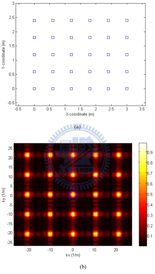
Initially, divisions (m = 24 and n = 30) of a square grid are set up on the microphone surface, as shown in Fig. 5 (a). Each side of the square grid measures 0.1m. The source frequency

m n×

f = 1.7 kHz and speed of sound m/s. The wave number k f

340

c= 2π / c 31.4

= = m-1_{. In addition, a URA of 5 (M = 30)} deployment with inter-element spacing = 0.6m is used as a benchmark in the following simulations, asshown in Fig. 5 (a). Its beam pattern calculated by Eq. (1) is shown in Fig. 5 (b). As expected, the grating lobes are clearly visible because the microphone spacing violates the λ/2-rule (d = 3λ at

6 ×

d

f = 1.7 kHz). The cost function calculated by Eq. (2) is only 1.0261 because of the grating lobes. This prompts the use of random deployment of microphones as follows.

In the MC simulation, the 30 microphones can freely occupy any 30 positions of the grid points on array surface. Exhaustive search would require

combinations for a 30-element array, while only 105 iterations are carried out using this MC search. The learning curve of the MC search with random arrays setting is shown in Fig. 6 (a). The search attains the optimal cost function 2.6532 at the 27596th iteration. The corresponding microphone positions and beam pattern are shown in Figs. 6 (b) and (c), respectively.

25 31×

4_×2814_×491

16 2

Beside the extremely time-consuming MC search, the SA approach is employed next. The annealing parameters of the SA for array deployment are chosen to be Ti =

10 deg K, Tf = 10-8 deg K and a=0.95 [14, 16]. The learning curve of the SA

search with initial random arrays setting (405 iterations) is shown in the left portion (denoted as 1stSA) of Fig. 7 (a). The curve fluctuates initially and then converges to a constant value 2.5767 between the 351st and the 405th iteration. The optimal microphone deployment and beam pattern are shown in Figs. 7 (b) and (c). In addition to optimizing the microphone positions, optimizing the microphone weights can further improve the value of the cost function.

On the basis of the configuration found previously by the SA, we continue to optimize the weights of microphones again using the SA algorithm. The number of iterations is increased to 1000. Starting from unity weights, the microphone weights are adjusted in each iteration with a random perturbation within the range of -0.1 to 0.1. The learning curve is shown in the right portion (denoted as 2ndSA) of Fig. 7 (a). The cost function is further increased to 2.7561 at the 1283rd iteration. The resulting beam pattern is shown in Fig. 7 (d), where a unique main-lobe is clearly visible.

Instead of the initial random arrays setting, the simulations using the MC and SA algorithms are also ran with initial URA setting. To save space, the results are only listed in Table 1.

2.3.2 Optimizing array deployment with IB constraint

In this section, the SA, IBMC and a combined SA-IBMC algorithm are exploited to optimize microphone deployment with the IB constraint. The MC search with IB constraint is particularly named IBMC in this thesis. In order to compare the efficiency of IBMC with MC, the preset run iterations are chosen to be 105, as the same number of MC simulation. The learning curve of the IBMC search with random arrays setting is shown in Fig. 8 (a). The search attains the optimal cost function 2.5638 at the 7662nd iteration. The corresponding microphone positions and beam pattern are shown in Figs. 8 (b) and (c), respectively.

Apart from the IBMC search, both microphone positions and weights are to be optimized using the SA algorithm. Specifically, the combined SA-IBMC method proceeds with three stages—the 1stSA stage, the IBMC stage, and the 2ndSA stage. The parameters of the two SA stages are identical to those in Section 5.1. The learning curve of the 1stSA stage (405 iterations) is shown in the left portion of Fig. 9 (a). The curve fluctuates initially and then converges to a constant value 2.5328

between the 208th and the 405th iteration. The resulting microphone deployment and beam pattern are shown in Figs. 9 (b) and (c). Being able to avoid local minima by accepting “bad” solutions in the initial SA search can be a benefit and shortcoming as well. It happens more often than never that the SA algorithm can miss the optimal solution in the initial stage and converge prematurely to a suboptimal one. A hybrid SA-IBMC approach is used in an attempt to address this problem.

The previous deployment obtained by the SA search is used as the input to the IBMC simulation. The microphone position can be randomly chosen from the nine grid points in the localized region. Each region necessarily contains one and only one microphone. Exhaustive search would require prohibitively 930 combinations for a 30-element array, while only 100 iterations are required in the IBMC search.

The learning curve of the IBMC (iteration 406-505) is shown in Fig. 9 (a). By the IBMC search, the cost function is further increased to 2.5465 at the 482nd iteration. Figures 9 (d) and (e) show the optimal microphone positions and beam pattern obtained at the 482nd iteration. Next, in the 2ndSA stage, the microphone weights are optimized based on the configuration found previously by the SA-IBMC approach.

The microphone weights initially set to unity are adjusted in each iteration with a random perturbation within the range of -0.1 to 0.1. The learning curve in 506 iterations is shown in Fig. 9 (a). The cost function is further increased to 2.6602 at the 1429th iteration. The resulting beam pattern is shown in Fig. 9 (f), where a unique main-lobe is clearly visible.

Apart from the URA, the random array deployment is also used as the initial setting in the simulation. For brevity, the results of MC, IBMC, SA and SA-IBMC simulations are summarized in Table 1. The simulation results obtained with and without the IB constraint are compared in terms of number of iterations and the maximum cost function values. Although the MC approach has reached the highest

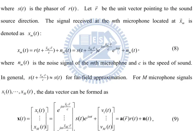
cost function (Q = 2.6532), it takes 27596 iterations to achieve this value. By comparing the results of the MC and IBMC (with the URA as the initial setting), we found that the IBMC approach can attain comparable cost function value to the MC approach with far less amount of computation (Q = 2.5638 at the 7662nd iteration of IBMC vs. Q = 2.6532 at the 27596th iteration of MC). In comparison with the results obtained using the SA algorithm with the IB constraint (Q = 2.6602 for the URA as the initial setting and Q = 2.6573 for a random array as the initial setting), the SA approach with no IB constraint has attained a slightly higher cost function (Q = 2.7561) with comparable computational complexity. It all boils down to the tradeoff between search time and optimality.

Incorporating the IB constraint could potentially have the following benefits. First, the IBMC algorithm is computationally more efficient than the plain MC algorithm because of smaller search areas. Second, in the hybrid SA-IBMC approach, the IB constraint could possibly improve the SA results when the SA algorithm converges prematurely to a suboptimal result. Third, the IB constraint normally results in uniform distributions of microphones. By “uniform”, we simply mean that microphones would not concentrate at only a few areas, which should not be confused with the deployment of the constant-spacing uniform arrays. In summary, it is fair to say that the IB constraint significantly reduces the computation complexity at the risk of converging to a suboptimal solution which may not be far from the global optimum. This is generally sufficient in practical applications.

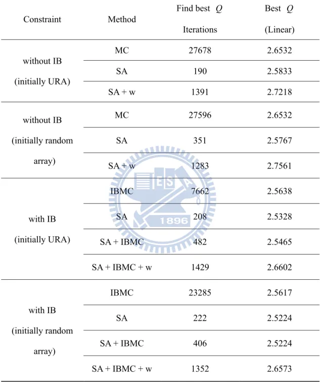
Apart from the source frequency 1.7 kHz, we also run the simulation for the other frequencies 500 Hz and 1 kHz. For brevity, we only summarize the results in Table 2. Random arrays yield unique main-lobe and higher cost function than the URA at the frequency 1 kHz. In lower frequency 500 Hz, no grating lobes are seen in the beam pattern of URA, while higher side-lobe level is found in the beam pattern

of the random array. This leads to a higher value of cost function for the URA than the random array at low frequencies.

3. Methods for Direction of Arrival (DOA) estimation

3.1 DAS algorithm

Before discussing DOA algorithms, an array model should be built. Considering an URA, the inter-element spacing is . Assume d r t( ) is a broadband frequency ω at a reference point:

( ) ( ) j t

r t =s t eω , (7)

where s t( ) is the phasor of r t( ). Let r be the unit vector pointing to the sound

source direction. The signal received at the mth microphone located at x is _m

denoted as x t : _m( ) ( ) ( m ) ( ) ( m ) m m m x r j x r x r _c j t c c m( ) x t r t n t s t e ω e ω n t ⋅ ⋅ ⋅ = + + = + + , (8)

where is the noise signal of the mth microhphne and c is the speed of sound. In general, ( ) m n t ( x rm ) ( c

s t+ ⋅ ≈s t) for far-field approximation. For M microphone signals

1( ), , M( )

x t x t , the data vector can be formed as

1 1( ) 1( ) ( ) ( ) ( ) ( ) ( ) ( ) ( ) M M M x r j c j t x r j c x t v t t r x t v t e s t e e ω ω ω ⋅ ⋅ ⎡ ⎤ ⎡ ⎤ ⎢ ⎥ ⎡ ⎤ ⎢ ⎥ ⎢ ⎥ ⎢ ⎥ =_{⎢ ⎥}=_{⎢ ⎥} +_{⎢ ⎥}= + ⎢ ⎥ ⎢ ⎥ ⎢ ⎥ ⎣ ⎦ ⎣ ⎦ ⎢ ⎥ ⎣ ⎦ x a r t n t , (9)

where a( r ) is called the array manifold vector.

Figure 10 illustrates a URA. There are I and J microphones with inter-element spacing dx and dy in the x and y axis, respectively. Let the left and the upper corner element is the reference point. The vector of pointing to each microphone from reference point in the polar coordinate is given as

( ) (( 1) ,( 1) ,0)

ij x y

x t = i− d j− d , (10)

where i = 1,2,…,I and j = 1,2,…,J. The unit vector r pointing for a sound source at the look directions θ and Φ is given by

(sin sin ,sin cos ,cos )

r = θ φ θ φ θ . (11)

The delay of each microphone will be given by

( 1) sin sin ( 1) sin cos

ij x y ij x r i d j d c c θ φ θ τ = ⋅ = − + − φ. (12)

Then the array manifold vector can be written as

sin sin

( 1) sin sin

sin cos

sin sin sin cos

( 1) sin sin ( 1) sin cos 1 ( , , ) x x y x y x y d j c I d j c d j c d d j c I d J d j c e e a e e e θ φ ω θ φ ω θ φ ω θ φ θ φ ω θ φ θ ω ω θ φ − + − + − φ ⎡ ⎤ ⎢ ⎥ ⎢ ⎥ ⎢ ⎥ ⎢ ⎥ ⎢ ⎥ ⎢ ⎥ ⎢ ⎥ = ⎢ ⎥ ⎢ ⎥ ⎢ ⎥ ⎢ ⎥ ⎢ ⎥ ⎢ ⎥ ⎢ ⎥ ⎢ ⎥ ⎣ ⎦ . (13)

With reference to the Fig. 11, the output of DAS beamformer is defined as

0 1 ( , ) M _m( _m) m y t θ x t τ = =

∑

− , (14) where ( )x t_m m

is the signal received by mth microphone, as shown in Eq. (9). In Eq. (14), τ are the steering delays appropriate for focusing the array to the look direction,θ₀, and compensation for the direct path propagation delay associated with the desired signal at each microphone.

In this thesis, the planar waves of far-field assumption are considered to be spherical waves because the waves are not really comes from infinite distances. Consequently, the delay of each channel in Eq. (14) can be calculated by

m m

x c

τ =Δ , (15)

where Δx_m is the distance between reference source positions θ_s and mth microphone. However, the delay usually is not an integer number in the digital processing. There are many ways to deal with the fractional delay problem. The simplest approach is Lagrange interpolation [29]. By multiplying τ_m by sampling frequency f , we can acquire the fractional delay _s ψ_m including integral component

and fractional component , respectively. The decomposition is illustrated as

m

D e_m

m fs m Dm em

τ ⋅ =ψ = + . (16)

For simplicity, the FIR filter coefficients are obtained from Eq. (17) to realize the Lagrange interpolation. 0 , 0,1, 2, N m mk l l k e l w k k l = ≠ − = = −

∏

_{N . (17)}

The coefficients for the Lagrange filters of order N=1, 2 are given in the Table 3. The case N=1 corresponds to linear interpolation between two samples. In our decision, the case N=2 is employed.

3.2 TR algorithm

The TR algorithm is simply based on an idea of reversing the received signal. Figure 12 shows the block diagram of TR algorithm. First, use a microphone array to receive and save sound data. The signal x(t) is reversed to x(-t) by TR block. Then the reversed signal x(-t) is played by a loudspeaker array.

3.3 SIMO-ESIF algorithm

The central idea of the proposed SIMO-ESIF algorithm is introduced in this section. In Fig. 13, M microphones are employed to pick up the sound emitting from

a source positioned in the far-field.

In the frequency domain, the sound pressure received at the microphones and the source signal can be related by a M× transfer 1 matrix H

( )

q ω

=

p H , (18)

where q( )ω is the Fourier transform of a scalar source strength,

[

1( ) ( )

]

T M p ω p ω = p

[

is the pressure vector with “T” denoting matrix transpose, and

]

1( ) ( ) T M h ω h ω =

H is theM× propagation matrix. The aim here is to estimate 1 the source signal q(ω based on the pressure measurement p by using a set of ) inverse filters

[

1( ) ( )

]

T M c ω c ω = C (19)

such that _{C H I}T _{≈ and therefore}

ˆ T T

q= C p C Hq q= ≈ . (20)

On the other hand, this problem can also be written in the context of the following least-squares optimization problem

2 2

min

q p - Hq , (21)

where ₂ denotes vector 2-norm. This is an overdetermined problem whose least-squares solution is given by

1 2 2 ˆ ( ) H H H q= H H H p− H p H = _{, (22)}

where the superscript “H” denotes hermitian transpose. Comparison of Eqs. (20) and (22) yields the following optimal inverse filter

2 2 H T ₌ H C H , (23)

“phase-conjugated” filters, or the “time-reversed” filters in the free-field context. Specifically, for a point source in the free field, it is straightforward to show that

2 2 2 1 1 M m= rm =

∑

H , (24)

where rm is the distance between source and the mth microphone. Since

2 2 H is a frequency-independent constant, the inverse filters and the time-reversed filters differ only by a constant. In a reverberant environment, these filters are different in general. Being able to incorporate the reverberant characteristics in the measured acoustical plant model represents an advantage of the proposed approach over conventional methods such as the DAS beamformer.

In real-time implementation, the inverse filters are converted to the time-domain finite-impulse-response (FIR) filters with the aid of inverse fast Fourier transform (IFFT) and circular shift. Thus, the source signal can be recovered by filtering the pressure signals with the inverse filters c(k):

ˆ( ) T( ) ( )

q k = c k ∗p k , (25)

where k is discrete-time index, c(k) is the impulse response of the inverse filter, and “*” denotes convolution.

3.4 Minimum Variance Distortionless Response (MVDR)algorithm

Another approach has been proposed using the data covariance matrix. This method has been shown to provide higher resolution in DOA estimations than the DAS algorithm. In order to facilitate digital processing, we simultaneously sample all array inputs to form digital data x t_m( )=x kT k_m( ), =1, 2, . For D sources, we may invoke principle of superposition to write

1 1 1 ( ) ( ) ( , ) ( ) ( ) [ ( , ) ( , )] ( ) ( ) ( ) ( ) D i j i i j r k k r k k r k k k ω θ ω θ ω θ = ⎡ ⎤ ⎢ ⎥ = + = _{⎢ ⎥} ⎢ ⎥ ⎣ ⎦ = +

∑

x a n a a n Ar n k + , (26)

where θ_i is the direction of the ith source, r(k) is the source signal vector and A is DOA matrix. A beamformer output is a linear combiner that produces an output signal by weighting and summing all components.

1 ( ) M ( ) H ( ) m m m y k w x k∗ = =

∑

=w x k , (27)

where w is the weight vector given by . Because the MVDR method exploits the correlation between array input signals, it is necessary to calculate the array signal correlation matrix.

1 [ ]T M w w = w

{

( ) H( )

}

xx =E k k R x x . (28)

Suppose that the noise is uncorrelated with signals _E

{

_r( )_{k n}H( )_k

}

₌0 _{and the noise} is spatially white

{

_{( )} H_{( )}

}

2

n

E n k n k =σ I . By the preceding assumption, the Eq. (28)

can be rewritten as

{

} {

}

2 ( ) H( ) ( ) H( ) xx H rr nn H rr n E k k E k k σ = + = + = + R A r r n n AR A R AR A I , (29)

where Rrr and Rnn are the source and noise correlation matrices, respectively. In practice, the data correlation matrix Rxx is usually approximated by the data covariance covariance

( ) H (1 ) ( 1), 1, 2 , (0)

xx p =α p p+ −α xx p− p= P xx

R x x R R = 0. (30)

At this recursive equation, α is a constant which satisfied 0≤ ≤α 1 [

. The received signal is divided to p frames and rearranged to the data vector x= x x_{1 2} x_p].

In the following, the aim is to find the MVDR weight vector w_MV . An optimization problem is given for solving the unknown vector w_MV. The MVDR beamformer attempts to minimize the output power

{

2

}

{

2

}

( ) H ( ) H

MV MV xx

E y k =E w x k =w R w_MV . (31) Another constraint is to maintain unity in the look direction . The

MVDR beamforming suppresses the undesired interference from

0 ( ) 1 H MV θ = w a 0 θ θ≠ and the noise. The problem can be expressed as follows

0 min subject to ( , ) 1 MV H MV xx MV MV ω θ = w w R w w a . (32)

This problem can be solved by Lagrange multiplier method

0 0 [ ( , ) 1] ( , ) 1 MV MV H MV xx MV MV MV λ ω θ ω θ ⎧∇ − ∇ ⎪ ⎨ = ⎪⎩ w w R w w w a w a 0 − = . (33)

If Rxx is nonsingular, Rxx can be inversed to solve the unknown vector by

1 0 ( , ) MV λ xx ω θ − = w R a , (34) where ₁ 0 0 1 ( , ) ( , ) H MV xx MV H xx λ ω θ − ω =w R w =

a R a θ is the beamformer output power.

Then λ is substituted in Eq. (34) to obtain the MVDR weight

1 0 1 0 0 ( , ) ( , ) ( , ) xx MV H xx ω θ ω θ ω − − = R a w a R a θ . (35)

In the preceding results, it is convenient to obtain the spatial power spectrum S_MV( )θ by continuing altering θ 1 1 ( ) ( , ) ( , ) H MV MV xx MV H xx S θ ω θ − ω =w R w = a R a θ . (36)

The spatial power spectrum S_MV( )θ exhibits J peaks approximately at θ₁ θ_D.

3.5 Multiple Signal Classification (MUSIC) algorithm

signals, an approach of DOA estimation has been proposed by exploiting the eigenvalue decomposition (EVD) of the covariance matrix. Firstly, the array covariance matrix Rxx in Eq. (30) is represented by EVD

2 H xx rr σn 1 − = + = R AR A I UΛU , (37)

where U is a unitary matrix and comprise M linearly independent eigenvectors

1 M

u …u . The eigenvector associate with M eigenvalues α₁ α_M . The array correlation matrix can be represented as

1 1 1 2 2 1 2 1 0 0 0 0 [ ] 0 0 H xx H H M H M m m m m H M M α α α α − = = = ⎡ ⎤ ⎡ ⎤ ⎢ ⎥ ⎢ ⎥ ⎢ ⎥ ⎢ ⎥ = = ⎢ ⎥ ⎢ ⎥ ⎢ ⎥ ⎢ ⎥ ⎢ ⎥ ⎣ ⎦ ⎣ ⎦

∑

R UΛU UΛU u u u u u u u u . (38)

The diagonal terms of Λ have been arranged with α α₁≥ ₂ ≥ ≥α_M. The noise term 2 n σ I can be yielded to 2 2 1 2 2 1 M H H n n n n m m σ σ − σ σ = = = =

∑

I UU UU u u_m . (39)

Because A consists of D sources, we assume that A and Rrr are of full rank D. Subsequently the signal-only correlation matrix Cxx is generated by subtracting the noise component from Rxx

2 1 ( ) M H H x x rr m n m m α σ = = =

∑

− C AR A u u_m . (40)

If Rrr is rank D and small than the array size M, the smallest M D− eigenvalues

1

D M

α ₊ α are equivalent to the noise power. Therefore the range of Cxx are spanned by u₁ to u . If the array has no coherent source between any of two _D

received signals, Rrr only has nonzero values on the diagonal terms which reprensent the power of the D sources. Note that the range of Cxx is identical to the range of A which is spanned by the manifold vectors a( , )ω θ₁ a( ,ω θ_D). The relation between

Cxx and A is

{ }

span ( , ), , ( ,

{

1 D)

}

span

{

1, , D

}

R A = a ω θ a ω θ = u u M u (41) and

{ }

span

{

D1, ,

}

R A ⊥ = u ₊ , (42)

where span

{

u₁, ,u_D

}

and span

{

u_D+1, ,u_M

}

M

are called the signal subspace and noise subspace, respectively. Because the subspace is orthogonal to the noise subspace such that

( , ) 0, 1, 2, , ; 1, 2, ,

s H

m ω θd = ds = D m D= + D+

u a . (43)

The MUSIC technique is to exploit Eq. (43) to improve the DOA estimations. The eigenvectors u_D+1, ,u is used to construct the projection matrix as follows _M

1 M H m m N m J= + =

∑

u u P . (44)

From Eq. (43), the direction of the source θ_i (i=1, , )D can be found by solving

1 ( , ) ( , ) , s M H N m m m J d ω θ ω θ = + =

∑

= P a u u a 0 θ θ= N . (45)

The projection matrix has the properties of 2 H N = N and N =

P P P P . The problem of

Eq. (45) can be extended to solve Eq. (46) for simplicity.

2 2

( , ) ( , )H H ( , ) 0,

N ω θ = ω θ N N ω θ θ i

P a a P P a = = . (46) θ

Equivalently, the inverse of Eq. (46) has the infinitely value when θ θ= _i, i=1, ,D. The inverse of Eq. (46) is denoted as MUSIC spectrum.

1 ( ) ( , ) ( , ) MU H N S θ ω θ ω = a P a θ . (47)

The peaks of the MUSIC spectrum are the directions of sources. Not that the MUSIC spectrum does not exhibit infinitely high peaks due to noises in practice. How to determine D is a problem. It would rather be overestimated than

choose D. By the spirit of AIC is to calculate matching error and weight the

truncated order, the equation can be defined as

1 ( ) ( ) , ( ) m H xx xx _F A xx i i i i AIC m ∗ m w m ∗ m α = = R −R + R =

∑

u u . (48)

The EVD of data covariance matrix is used to calculate the matching error, which is ( )

xx xx m _F

∗

−

R R . The weight part is to weight order by w in order to make the _A

order with lowest AIC value would be the same order in the error line which has an apparent turning point. For a preset two point sources simulation, the error, weight and AIC lines are shown in Fig. 14 (a). From the figure, the turning point of error line is at the 4th order. Thus the weight w should be chosen to make the AIC line _A

will have a lowest point at that order. In our simulation, the value is chosen to be 0.5*10^12. Figure 14(b) shows the AIC line with different weight.

3.6 Numerical simulations of DOA algorithms

In order to validate and compare the several methods of DOA estimation, numerical simulations are conducted for a 30-channel URA and a random array optimized by SA-IBMC optimization method. The aperture of array is 0.4m×0.5m (d = 0.1m) for URA and 0.5m×0.6m for random array, as shown in Figs. 15 (a) and (b).

There are two simulated whitenoise sources located at the positions (-0.5m, 0.5m) and (0.5m, -0.5m). The sources are 1m from array surface. Assume the sound velocity

cs is 343 m/s. Consider the λ/ 2 rule, the maximum measurement frequency with inter-element spacing 0.1m is f_max =c/ 2d =1.7 kHz

/ 4

d

. Therefore, we choose point sources with the frequencies 1 kHz ( =λ ) and 7 kHz (d =2λ) to be the observed frequencies in simulations. The magnitude of beam pattern or spectrum of each approach is normalized to a range from 0 to 1. This makes the results of five methods can easily be compared in main-lobe width and side-lobes levels.

Figures 13 (a)-(j) illustrate the noise maps of two simulated point sources obtained using different acoustic imaging algorithms with a URA or an optimized random array in the frequency 1 kHz. At this frequency, the spacing is less than a half of wave length. Therefore, grating lobes are not occurring in the simulated results of URA and random configurations. The noise maps obtained using DAS and TR algorithms are shown in Figs. 13 (a)-(d). Both of these figures are with poor resolution. They have very large main lobes but cannot correctly point the preset source positions. The noise maps of another lower resolution algorithm SIMO-ESIF is shown in Figs. 16 (e) and (f). Compared with results of DAS and TR, SIMO-ESIF also has large main lobes but can correctly point the source positions. Figures 16 (g)-(j) show the noise maps obtained using MVDR and MUSIC algorithms with two array configurations. As predicted, the results validated that the MVDR and MUSIC are the methods which can achieve higher resolutions, especially MUSIC. They can correctly localize the preset source points with narrow main lobes. The side-lobes of MVDR are higher than MUSIC.

Apart from simulations at frequency 1 kHz, we also run some simulations in a higher frequency to make the spacing exceeds a half of a wave length. Clearly, the frequency is chosen to be 7 kHz. At this frequency, the spacing is approximate two times of a length. Figures 14(a)-(j) show the noise maps of two simulated point sources of DOA estimation using different approaches with a URA and an optimized random array in the frequency 7 kHz. The simulated results are largely identical but minor differences with the results in the frequency 1 kHz except the grating lobes appeared at those power spectrums with URA configuration. In SIMO-ESIF and MUSIC cases, the noise maps have no clearly visible grating lobes with URA configuration. Nevertheless, the noise maps obtained using SIMO-ESIF still have large main lobes and much higher side lobes than MUSIC. Summary, the MUSIC is

the algorithm which can obtain highest resolution in the frequency from low to high. The MVDR is worse than MUSIC but still can get relatively higher resolution than other algorithms. The proposed SIMO-ESIF is the only in low resolution algorithms which can use URA to localize high frequency noise sources. The comparisons of these five acoustic imaging algorithms are illustrated in Table 4.

4. Experimental verifications

To validate the MUSIC algorithm, practical sources including loudspeakers, a compressor and a scooter were chosen as the test targets for experiments. Figure 18 shows the beamformer properties at 30o opening angle. In our experimental arrangement, inter-element spacing d =0.1m array aperture and distance between sources plane and microphone array surface . Assume sound velocity 0.5m A D = 1m z= 345m/s v

c = . The maximum and minimum measureable frequency can be calculated by min 4 3 2 v max v A c f d c f D = ⋅ = . (49)

From Eq. (49), the maximum and minimum measureable frequency is , respectively. The resolution R is

2.3 kHz and 690Hz 1.22 A z R D λ = _{. (50)}

And the area covered L is

1.15 .

L= z . (51)

Therefore, the resolution of frequency 1 kHz and 7 kHz is 0.84m and 0.12m, respectively. The area covered is 1.15m at distance z = 1m. Figure 19 shows the

experimental arrangement. In experiments, the array configurations are a 30-channe URA deployed as 5×6 and a 30-channel random array that was optimized in an informal numerical simulation. The URA with spacing 0.1m and optimized random arrayare deployed as Figs. 15 (a) and (b), respectively. Thirty array microphones, PCB 130D20, were used to make the sound pressure measurements. Two PXI 4496 systems [31] in conjunction with LabVIEW8.5 software [31] were used for data acquisition and processing.

4.1 Loudspeakers experiment

In loudspeakers experiments, two loudspeakers are situated at (0.1m, 0.2m) and (0.5m, 0.2m), respectively. These loudspeakers with whitenoise sources are situated at 1m far from array surface. The observed frequencies are chosen to be 1 kHz (d=λ/ 4) and 7 kHz (d =2λ), as the same frequencies in numerical simulations. Figures 20 (a)-(j) show the noise maps obtained using five acoustic imaging algorithms with random array configuration at frequency 1 kHz. In this low frequency, the distance between loudspeakers is 0.4m. The distance is small than the resolution R = 0.84m calculated by Eq. (50). Therefore, it cannot localize the two

too closer noise sources with either URA or random array configuration. But in high resolution MVDR and MUSIC algorithms, it perhaps distinguishes the two sources.

For higher frequency experiments, the noise maps are shown in Figs. 21 (a)-(j). Obviously, grating lobes occur at 7 kHz with the URA configuration. On the contrary, the experimental results using random array are well localized the source positions. The experimental results get the same summary with numerical simulations.

4.2 Compressor experiment

A compressor is chosen to be a more practical sound source in measurements using the optimized random array. The compressor is mounted on a table inside a semi-anechoic room. In deployment, the compressor is located in 1m from array surface. The observed frequency is chosen to be 1 kHz. The noise map obtained using MUSIC algorithm with the optimized random array is shown in Fig. 22. The major noise is found at the air intake position.

In this experiment, a 125cc scooter served as a more practical source to examine the capability of MUSIC in DOA estimation with non-stationary sources. The scooter is mounted on a dynamometer inside a semi-anechoic room. The distance between the scooter and array is 3m. The observed frequency is chosen to be 7 kHz. The MUSIC algorithm was used to estimate the DOA on the right side of the scooter in a run-up test. The engine speed increased from 1500 rpm to 7500 rpm within ten seconds. Figure 23 shows the noise map. From the figure, it revealed that the inlet and outlet of exhaust pipe were the major noise source positions.

5. Conclusion

There have two major researches in this thesis. First, optimized planar array deployment for source imaging is investigated in this thesis. Global optimization algorithms have been developed to facilitate the search of the optimized microphone deployment. The SA algorithm and the combined SA-IBMC algorithm prove effective in finding the optimal deployment. For far-field array with sparse deployment in which inter-element spacing is large, random deployment with optimal weights is crucial to avoid grating lobes. As predicted by the conventional wisdom, the optimized random sparse array has excellent beam pattern with a unique main-lobe. Second, several acoustic imaging algorithms including DAS, TR, MVDR, MUSIC and an inverse filter-based method SIMO-ESIF have been developed to estimate DOA. The resolutions of noise maps in low frequency are much worse than in high frequency with random array configuration. The proposed SIMO-ESIF approach can use URA to estimate DOA in high frequency without grating lobes problem. As expected, the high resolution methods such as MVDR and MUSIC can obtain much greater results than DAS, TR and SIMO-ESIF in localizing sound source positions.

REFERENCES

[1] M.I. Skolnik, Introduction to Radar Systems, McGraw-Hill, New York, 1980.

[2] A.V. OPPENHEIM and R.W. SCHAFER, Discrete-Time Signal Processing, Prentice-Hall, Englewood Cliffs, NJ, 1989.

[3] S. Haykin, Array Signal Processing, Prentice Hall, Englewood Cliffs, NJ, 1985.

[4] H.T. FRIIS and C.B. FELDMAN, A multiple unit steerable antenna for short-wave reception, Bell Syst. Tech. J. 16 (1937) 337-419.

[5] P. T. SODERMAN and S. C. NOBLE, Directional microphone array for acoustic studies of wind tunnel models, J. Aircr., 12 (1975) 168-173.

[6] S.F. WU, On reconstruction of acoustic pressure fields using the Helmholtz equation least squares method, Journal of the Acoustical Society of America 107

(5) (2000) 2511-2522.

[7] E.G. WILLIAMS, J.D. MAYNARD and E. SKUARZYK, Sound source reconstruction using a microphone array, Journal of the Acoustical Society of America 68 (1980)

340-344.

[8] S. CHRISTOPHER, Numerical annealing of low-redundancy linear arrays, IEEE Trans.

Antenna and Propagation 41 (1) (1993) 85-90.

[9] N. METROPOLIS and S. ULAM, The Monte Carlo method, J. American Statistical

Association 44 (1949) 335–341.

[10] J.M. HAMMERSLEY and D.C. HANDSCOMB, Monte Carlo methods, Chapman and Hall, London, 1979.

[11] F. DELLAERT, D. FOX, W. BURGARD, and S. THRUN, Monte Carlo localization for mobile robots, IEEE International Conference on Robotics and Automation, An Arbor (1999) 1322-1328.

[12] A. BAGGIO and K. LANGENDOEN, Monte Carlo localization for mobile wireless sensor networks, Ad Hoc Networks 6 (2008) 718-733.

[13] G. MARMIDIS, S. LAZAROU and E. PYRGIOTI, Optimal placement of wind turbines in a wind park using Monte Carlo simulation, Renewable Energy 33 (2008)

1455-1460.

[14] S. KIRKPATRICK, C.D. GELATT, C.D. JR, and M.P. VECCHI, Optimization by simulated annealing, Science 220 (4598) (1983) 671-680.

[15] R.T. EDUARDO, J.K. HAO and T.J. JOSE, An effective two-stage simulated annealing algorithm for the minimum linear arrangement problem, Computer and Operation Research 35 (2008) 3331-3346.

[16] B. FRANCO, Simulated Annealing Overview. http://www.geocities.com/ francorbusetti, 2003 (last viewed, June 20, 2009).

[17] V. MURINO, A. TRUCCO, and C.S. REGAZZONI, Synthesis of unequally spaced arrays by simulated annealing, IEEE Trans. Signal Processing 44 (1) (1996) 119–123.

[18] A. TRUCCO, Thinning and weighting of large planar arrays by simulated annealing,

IEEE Trans. Ultrasonics, Ferroelectrics, and Frequency Control 46 (2) (1999)

374-355.

[19] H. L. Van Trees, Optimum array processing: part IV of detection, estimation, and modulation, John Wiley & Sons, Inc., New York, 2002.

[20] J.J. CHRISTENSEN and J. HALD, Beamforming, Brüel & Kjær Technical Review No.

1, 2004.

[21] M.R. BAI, and J.H. LIN, Source identification system based on the time-domain nearfield equivalence source imaging: fundamental theory and implementation,

Journal of Sound and Vibration 307 (2007) 202–225.

[22] J. CAPON, High-resolution frequency-wavenumber spectrum analysis, Proc. IEEE 57 (1969) 1408-1418.

[23] B. JOCOB, J. CHEN and Y. HUANG, A generalized MVDR spectrum, IEEE Signal

[24] C.L.NIKIAS and J. M. MENDEL, Signal processing with higher order spectra, IEEE

Signal Processing Magazine, (1993) 10-37.

[25] R.O. SCHMIDT, Multiple emitter location and signal parameter estimation, IEEE

Trans. Antennas and Propagation AP-34 (3) (1986) 276-280.

[26] M.R. BAI and J.W. LEE, Industrial noise identification by using an acoustic beamforming system, ASME, Journal of Vibration and Acoustics 120 (1998)

426-433.

[27] Y. T. CHO and M. J. ROAN, Visualization of bearing noise using adaptive high-resolution near-field beamforming, J. Mechanical Engineering Science, 223

(2008), 1339-1349.

[28] M.R. GAREY and D.S. JOHNSON, Computers and Intractability: A Guide to the

Theory of NP-Completeness, W. H. Freeman and Company, San Francisco, 1979.

[29] T. LAAKSO, V. VALIMAKI, M. KARJALAINEN and U. LAINE, Splitting the unit delay,

IEEE Signal Processing Magazine, 1996.

[30] HIROTUGU, AKAIKE, A new look at the statistical model identification, IEEE

Transactions on Automatic Control 19 (6) (1974), 716-723.

[31] National Instruments Corporation, PCI extensions for Instrumentation (PXI) http://www.ni.com/ (last viewed, November 15, 2008).

Table 1. The search performance of different optimization methods for array deployment with the inter-element spacing d = 0.6 m (3λ at the frequency

1.7 kHz). The letter “w” indicates that weight optimization is performed.

Constraint Method Find best Q Iterations Best Q (Linear) without IB (initially URA) MC 27678 2.6532 SA 190 2.5833 SA + w 1391 2.7218 without IB (initially random array) MC 27596 2.6532 SA 351 2.5767 SA + w 1283 2.7561 with IB (initially URA) IBMC 7662 2.5638 SA 208 2.5328 SA + IBMC 482 2.5465 SA + IBMC + w 1429 2.6602 with IB (initially random array) IBMC 23285 2.5617 SA 222 2.5224 SA + IBMC 406 2.5224 SA + IBMC + w 1352 2.6573

Table 2. The comparison of converged cost function Q of the URA and the optimized

random arrays at three different frequencies.

Array f = 500 Hz (d =λ) f = 1 kHz (d =1.75λ) f = 1.7 kHz (d =3λ) URA 4.0216 1.0192 1.0261 Random array

(without IB, initially URA) 2.5459 2.5459 2.7218

Random array

(without IB, initially random array)

2.5961 2.5451 2.7561

Random array

(with IB, initially URA) 2.5048 2.3324 2.6602

Random array

Table 3. Lagrange interpolation FIR filter coefficients for N = 1 and N = 2 wm0 wm1 wm2

N = 1 1 - em em

Table 4. Comparisons of acoustic imaging algorithms.

DAS TR SIMO-ESIF MVDR MUSIC

algorithm delay-sum time-reversed inverse filtering

MVDR MUSIC

resolution low low low high very high

complexity low low low high high

area covered large large small/large large large processing

domain

time time frequency frequency frequency

frequency range

high high low/high low/high low/high

sample/batch sample batch batch batch batch robustness to

reverberation

poor high high low low

acoustic variables