寬頻光射頻頻譜分析儀

全文

(1)國立交通大學光電工程研究所碩士論文. 高頻光射頻頻譜分析儀 High Bandwidth Optical RF Spectrum Analyzer. 研究生: 指導教授:. 林峰生祁甡. 教授. 陳智弘助理教授. 中華民國九十三年六月.

(2) 高頻光射頻頻譜分析儀. High Bandwidth Optical RF Spectrum Analyzer. 研究生 : 林峰生指導教授 : 祁甡教授陳智弘助理教授. Student : Feng-Sheng Lin Advisor: Prof. Sien Chi Assist. Prof. Zhi-Hong Chen. 國立交通大學光電工程研究所碩士論文. A Thesis Submitted to Institute of Electro-Optical Engineering College of Electrical Engineering and Computer Science National Chiao Tung University In Partial Fulfillment of the Requirements For the Degree of Master In Institute of Electro-Optical Engineering June 2004 Hsinchu, Taiwan, Republic of China. 中. 華. 民. 國. 九. 十. 三. 年. 六. 月.

(3) 致謝 ACKNOWLEDGEMENTS. 碩士班的日子像眨眼般, 不覺中即將結束了. 一直覺得自己運氣非常地好, 身邊總是圍繞著良師與益友. 首先, 非常感謝祁甡老師提供了我一個這麼設備完善的研究環境, 祁老師的寬宏大度的處世態度也是令我們非常感佩的, 而我也才能順利完成這篇論文. 還有陳智弘老師, 能遇到老師, 接受老師的指導, 我的運氣真的很好. 老師除了在實驗上盡心盡力地給予我們指導之外, 在處世態度上也給予我們很多的啟發與示範. 真的很少遇到像老師這麼平易近人且為學生著想的老師, 老師謝謝您. 碩士班這段日子真的學到了蠻多東西的, 謝謝您們, 兩位老師. 此外, 還有實驗室的學長姐們—林玉明博士, 彭朋群學長, 彭煒仁學長, 明芳學姊…, 謝謝你們不吝惜分享你們的經驗給我, 讓我能更快地進入狀況. 以及實驗室裡, 一起努力的同學們—家健, 宥燁, 建宏, 偉至, 馥宇, 盈傑, 嘉和, 至洋…謝謝你們在這段期間給我的幫助, 與我一起討論. 最後, 謝謝我的家人們以及許多陪伴我度過壓力最大的那段日子的朋友們.. 峰生 2004.5.24. i.

(4) 高頻光射頻頻譜分析儀. 學生 : 林峰生. 指導教授 : 祁甡. 教授. 陳智弘助理教授. 國立交通大學光電工程研究所碩士班. 摘要. 隨著光通訊系統的傳輸速率的增加, 傳統量測光通訊信號的方法漸漸地顯得局促了. 由於這些傳統的方法是將光通訊訊號先轉為電信號, 再由電的分析儀器, 來分析, 所以, 受到了光轉電以及分析儀器電子電路頻寬的限制. 其中, 信號的射頻頻譜是一個很重要且基本的量測. 一般電的射頻頻譜分析儀, 其頻寬限制約在 50GHz, 對於 40Gbps 的光通訊信號而言, 以顯不足. 為此, Dorrer 博士和 Maywar 博士在 2003 年提出了一個全光量測光信號射頻頻譜的方法. 這是一個簡單而且對於往後高傳輸速率的光通訊系統深具潛力的射頻頻譜量測方法. 我們對它非常感興趣, 因此依循 Dorrer 博士和 Maywar 博士的方法, 架設了如此一個光射頻頻譜分析儀. 並且, 仔細討論了它的工作原理以及相關的理論, 包括模擬量測的頻譜, 以之與實驗的結果比較, 並預測此方法因為信號光能量過大造成的誤差, 找出較適合的操作. ii.

(5) 除此之外, 我們以實驗以及理論模擬預測了所架的光射頻頻譜分析儀其具有的頻寬. 在不考慮頻譜展開以及信號重疊的情況下, 它具有約 750GH 的頻寬, 比電的射頻頻譜分析儀高出了一個數量級. 最後, 我們討論了此種全光光射頻頻譜分析儀的主要缺點—測量解析度的問題, 並建議了幾種改進的方法.. iii.

(6) High Bandwidth Optical RF Spectrum Analyzer. Student: Feng-Shen Lin. Advisors: Prof. Sien Chi Assistant Prof. Zhi-Hong Chen. Institute of Electro-Optical Engineering National Chiao Tung University. ABSTRACT. The conventional approach for measuring the optical communication signals is too restricted when the higher optical communication systems come. These conventional approaches are to convert the optical signal into electrical signal first and then do analysis by electrical instruments, so they are restricted by the optical-to-electrical conversion and electrical circuits in bandwidth. One of important and basic measurements for communication signals is to measure its RF spectrum. The largest bandwidth for general electrical RF spectrum analyzer is around 50GHz, which is insufficient for the measurement of 40Gbps optical communication signals. Therefore Dr. Dorrer and Dr. Maywar proposed an all optical approach for measuring the RF spectrum of optical signals in 2003. It is a simple method and has large potential for high bit rate optical communication. iv.

(7) systems. We have great interest in this all optical approach, so we set build up an optical RF spectrum analyzer based on the approach proposed by Dr. Dorrer and Dr. Maywar. Furthermore we discuss its working principle and the related theories including simulating the spectrum that we prepare to measure and compare it with the practical measured results. And predict the distortion due to too large signal power in this approach and find a suitable signal power in operation. Beside those, we still predict the achievable bandwidth of the optical RF spectrum analyzer with experiment and simulation. It has the largest bandwidth around 750GHz in the case without considering spectral extending and signal overlapping. Finally we discuss the major drawback of this approach—bad measuring resolution and suggest several possible methods for enhancing the measuring resolution.. v.

(8) Contents. Acknowledgements. i. Chinese Abstract. ii. English Abstract. iv. Contents. vi. Lists of Figures. viii. List of Tables. xi. Chapter 1: Introduction. 1. Chapter 2: Design of the optical RF spectrum analyzer. 4. 2-1: Working principle of the “optical RF spectrum analyzer”— 4 Nonlinear intensity to field conversion (NLIFC) 2-2: Simulation of the optical spectrum of the reference wave after NLIFC— 10 Estimate the maximum signal power without distorting the RF spectrum Chapter 3: Setup of the optical RF spectrum analyzer. 27. 3-1: Required highly nonlinear fiber (HNLF). 27. 3-1-1: The measurement of its high nonlinear coefficient,γ. 28. 3-1-2: The measurement of its dispersion properties. 40. 3-1-3: Control and estimate the loss. 43. 3-2: Measurement results of 10Gbps RZ signal and 40GHz sinusoidal signal. 46. 3-2-1: 10Gbps RZ signal. 46. 3-2-2: 40GHz sinusoidal signal. 52. 3-3: Simulation for the measurement with OSA. vi. 56.

(9) Chapter 4: The performance of the optical RF spectrum analyzer. 64. 4-1: The bandwidth performance and optimization. 64. 4-1-1: The model considering the group delay between signal and 65 reference waves 4-1-2: The model considering the group delay inside the signal wave 4-2: The resolution consideration and enhancement. 72 85. 4-2-1: Enhancement with a mathematical deconvolution. 85. 4-2-2: Enhancement with a coherent heterodyne detection. 87. Chapter 5: Conclusion. 90. Reference. 92. vii.

(10) List of figures. Fig 1. Illustration of the working principle of optical RF spectrum analyzer. Fig 2. Illustration oft the simulation of generation of optical spectrum of reference light after HNLF. Fig 3. Pattern and eye diagram of the simulated 10Gbps signal under test (Pav=12.39mW). Fig 4. Optical spectrum of the signal light passing through the HNLF. Fig 5. RF spectrum of the signal under test. Fig 6. Difference between RF spectrum signals and the optical spectrum of the reference light. Fig 7. Compare the two optical spectrums (PI=12.39mW). Fig 8. Distortion in the case of 10Gbps signal with 12.39 mW input power. Fig 9. The optical spectrums and distortion in the case of 10Gbps signal with PI=4.2mW. Fig 10. The relation between the signal power and the 3-dB bandwidth. Fig 11. Pattern and eye diagram of the 40Gbps signal under test (Pav=12.39mW). Fig 12. Resulting spectrums for 40Gbps signal with PI=12.39mW. Fig 13. Difference between the RF spectrum and optical spectrum and distortion caused by the key approximation for 40Gbps signal. Fig 14. Spectrums of term1 and term2 in eq.2-12. Fig 15. Simulated MI gain coefficient (input laser with power=16dBm, λ=1559nm). Fig 16. Simulated MI gain spectrum (input laser with power=16dBm, λ=1559nm). viii.

(11) Fig 17. Experiment setup of the observation of the MI gain spectrum. Fig 18. MI gain spectrum (PI=16dBm,λ=1559nm). Fig 19. The MI gain spectrums. Fig 20. Left: The linear relation between gmax and PI Right: The linear relation between Δf 2 and PI. Fig 21. The value of γ, │ß2│ (D) and λ0. Fig 22. Dispersion properties of Corning HNLF measured by ADVANTEST Q7760 optical network analyzer. Fig 23. Dispersion properties of Corning HNLF. Fig 24. Setup of measuring the intrinsic loss of HNLF and splicing loss. Fig 25. A sketch of the optical RF spectrum analyzer. Fig 26. Experimental setup of the RF spectrum of 10Gbps signal. Fig 27. Eye of the signal under test before amplification. Fig 28. Eye of the signal under test after amplification and adjusting the DL. Fig 29. Measurement result of 10G signal power at 14.7dBm. Fig 30. Measurement result of 10G signal power at 10dBm. Fig 31. Measurement result of 10G signal power at 5dBm. Fig 32. Experimental setup of the RF spectrum of 40Gbps signal. Fig 33. 40GHz sinusoidal signal before amplification. Fig 34. 40GHz sinusoidal signal after amplification. Fig 35. Measurement result of 40G signal power at 19.1dBm. Fig 36. Measurement result of 40G signal at 15dBm. Fig 37. Measurement result of 40G signal at 10dBm. Fig 38. Measurement result of 40G signal at 5dBm. Fig 39. Simplified block diagram of OSA (extracted from [5]). ix.

(12) Fig 40. The assumed filter with bandwidth=1GHz and dynamic range=60dB. Fig 41. Optical spectrums of reference light for 10Gbps RZ signal with signal input power of 14.7dBm. Fig 42. Dynamic range of OSA. Fig 43. Optical spectrums of reference light for 40GHz sinusoidal signal with signal input power of 14.7dBm. Fig 44. Sketch map of phase mismatching. Fig 45. Bandwidth reduction function. Fig 46. ß1 and ß2 of the Corning HNLF. Fig 47. 3dB bandwidth versus the separation. Fig 48. Sketch map of the model considering the phase mismatching inside signal. Fig 49. The simulated bandwidth reduction operated at best arrangement based on the modified model. Fig 50. 3dB-bandwidth versus the separation between signal and reference lights. Fig 51. The explanation of additional fields generation and the spectral extending. Fig 52. The simulated bandwidth reduction operated involving condition-1 and condition2. Fig 53. 3dB-bandwidth versus the separation at various conditions. Fig 54. The experiment setup for measuring the bandwidth of the optical RF spectrum analyzer. Fig 55. Measured bandwidth reduction. Fig 56. The measured 3dB-bandwidth versus the separation. Fig 57. Simulated deconvolution result. Fig 58. Filter shape. Fig 59. Deconvolution result. Fig 60. Explanation of the heterodyne approach. x.

(13) List of tables. Table 1. Simulation parameters for 10Gbps signal. Table 2. Simulation parameters for 40Gbps signal. Table 3. Corning Highly Non-linear, Zero Dispersion @ 1550 Specialty Fiber. Table 4. Compression of measured results from MI gain spectrum and Q7760. Table 5. The best fusion conditions of for fusing the HNLF and SMF. Table 6. Experimental conditions for 10Gbps signal. Table 7. Comparison of some characteristics of signal before and amplification. Table 8. Experimental conditions for 40Gbps signal. Table 9. Parameters in the simulation of OSA measurement process. Table 10. Some symbols used in this model. Table 11. The six four-waves mixing fields. Table 12. Features of the optical RF spectrum analyzer. xi.

(14) Chapter One. Introduction. Motivation. The bit rate of optical communication system is increasing. Now 40 Gbps long haul systems are commercially available, and higher bit rate system will come in the future. Thus there will be a trouble coming with these high bit rate communication systems—the lack of high speed diagnostics. One of useful diagnostics is to measure the RF spectrum of the signal under test, which is the power spectrum of the signal intensity. It is measured through a fast photo detector and an electrical super-heterodyne RF spectrum analyzer in optical communications. This kind of approach has limited bandwidth (~50GHz) due to the bandwidth limitations of the photo detector and the electronics in RF spectrum analyzer. Thus even for the 40Gbps system, the commercial electrical spectrum analyzer is inefficient in bandwidth for observing the second harmonics of the 40Gbps signal. Fortunately, there is an interesting approach for measuring the RF spectrum of the high bit rate optical signal proposed by C. Dorrer and D.N. Maywar in 2003 [1, 2, and 3]. And, this new method is an all optical approach, so it avoids the bandwidth limitation from the optical-to-electrical conversion and electronics and has an amazing large bandwidth (~750GHz).. Outline. In the thesis, an all optical RF analyzer followed the approach of C. Dorrer and 1.

(15) D.N. Maywar is repeated and the related theories, simulations and discussions are also involved. Further, we suggest some methods to overcome the biggest drawback of this approach—bad measuring resolution. Although this new all optical approach for measuring the RF spectrum of an optical communication signal has a very larger bandwidth than the conventional electrical RF spectrum analyzer, its measurement resolution is still too bad, which depends on the light frequency resolving instruments. In the setup of Dr. Dorrer and Dr. D.N. and ours, an OSA is used to resolve the reference light after nonlinear interaction, so the resolution is determine by the OSA and around 1GHz. There are several methods for improving the resolution are discussed in this thesis. In chapter two, we state the basics of the optical RF spectrum analyzer including the derivation of its working principle—the nonlinear intensity to field conversion (NLIFC) and simulating the optical spectrum of the reference wave after NLIFC that is useful for further discussions. Because this approach is based on the nonlinear intensity to field conversion, which is formed by cross phase modulation (XPM), the theories of XPM and how the NLIFC realizes our desire will be considered in section 2-1. And in section 2-2, we explain how a simulated optical spectrum of a reference wave after NLIFC is produced and show that it is similar to the RF spectrum of the original signal under test. Further, we will consider the distortion originated from the key approximation of this approach. In chapter three, we will build up the optical RF spectrum analyzer. Some important parameters will be measured including the nonlinear coefficient of the HNLF and its dispersion properties and loss, which are in section 3-1. And, the section 3-2 describes the practical measurements of the RF spectrum of signals. Then, we will do the simulation of OSA measurement in section 3-3. We will find that the simulated and experimental results are similar. 2.

(16) In chapter four, we discuss the performance of the optical RF spectrum analyzer. The performance of the optical RF spectrum analyzer includes the bandwidth performance that is discussed in section 4-1, and the resolution performance that is contained in section 4-2. In section 4-1, we will discuss the reasons causing the bandwidth degradation of the NLIFC and our optical RF spectrum analyzer based on NLIFC. We will have some analytical models to predict the bandwidth degradation and the best operation condition (to have largest measuring bandwidth). Because the major drawback of this new approach for measuring the RF spectrum of an optical signal is that the measurement resolution of this approach is much lower than that of the conventional electrical RF spectrum analyzer, we discuss some possible methods for improving the resolution in section 4-2. Finally, a conclusion is given in chapter five. Besides conclude the works that we done, we also compare the features of this all optical approach for measuring RF spectrum of a signal.. 3.

(17) Chapter Two. Design of the Optical RF Spectrum Analyzer. 2-1 Working principle of the “optical RF spectrum analyzer”— Nonlinear intensity to field conversion (NLIFC). This section explains the working principle of the optical RF spectrum analyzer with mathematical derivation.. “RF spectrum” and “Optical spectrum”. Before investigating how the “optical RF spectrum analyzer” works, we have to know the meanings and their differences between RF spectrum and optical spectrum. The “RF spectrum” of a communication signal is the power spectrum of the temporal intensity of the signal, I (t): 2. I RF (f) ≡ ∫ I(t)expi2π ft dt …eq. (2-1) It is the most popular measurement for investigating the communication signal in frequency domain with respect to the eye diagram in the time domain. It is very basic in the field of communication including optical communication and communication with other carriers. It is achieved through an electrical RF spectrum analyzer. And, we have to transfer the optical signal into electrical form by a fast photo detector. The measurement of an optical spectrum is to measure the power spectrum of the electric field of a light, E (t): I optical (f) ≡. 2. i2π ft ∫ E(t)exp dt …eq. (2-2). It is a physical parameter and obtained by an optical spectrum analyzer (OSA). 4.

(18) Nonlinear intensity to field conversion (NLIFC). In one word, this new approach uses a nonlinear interaction between signal light and reference light transferring the RF spectrum of the signal under test to the optical spectrum of the reference light observed. In fact, this nonlinear interaction that we use is a cross phase modulation (XPM) between signal and reference inside a high nonlinear fiber (HNLF). Through a proper choice of signal power and nonlinear coefficient—γ, we can transfer the nonlinear phase term containing the intensity information of signal light into the amplitude of the electric field of the reference light with a approximation. Thus, Dr. Dorrer and Dr. Maywar named the nonlinear interaction used in the new approach as “nonlinear intensity to field conversion (NLIFC)”. Following is a theoretical discussion about the NLIFC starting from XPM in a fiber. As to the related knowledge of the XPM in a fiber, it is introduced in [4]. Consider two lights propagating inside a fiber and suffering 3rd order nonlinear effect including XPM and SPM (self phase modulation). Because of the intensity dependent nonlinear refractive index—nI2 or n2, we can found that each of the two lights will obtain a nonlinear phase term dependent on the intensities of itself or the other co-propagating light after passing through the fiber. And, the nonlinear phase term can be represented as the eq. (2-3):. {. }. 2 2 ⎛ 2π f 0 j z ⎞ n2 j ⎟ E j + 2 E 3− j … eq. (2-3) ⎝ c ⎠. φ jNL = ⎜. The index j varying from 1 to 2 represents each light inside the fiber, E j is the amplitude of electric field of each light and n2 j is the nonlinear refractive index with 2. unit of reciprocal of E j , m2/V2. We can see that the nonlinear phase term is composed by SPM and XPM. 5.

(19) 2. For explaining the NLIFC, we rewrite the eq. (2-3) by replacing E j with intensity, I.. φ0NL =. 2π f 0 z I 2π f 0 z I 2π f 0 z I n 2 ( I 0 + 2 I (t ) ) = n 2 I0 + 2 × n 2 I (t ) c c c SPM. XPM. = φ0NL SPM. = φ0NL XPM. … eq. (2-4). In this equation, φ0NL is the nonlinear phase term suffered by the reference light after passing through the fiber, f 0 is the frequency of the reference light, I 0 is the intensity of the reference laser, and I ( t ) is the temporal intensity of the signal under test. As to. n2I , it is calculated around the frequency of reference light and related with n2 by following equation. n2I =. 2n2 ... eq. (2-5) ε 0cnL 2. , which is due to the unit conversion between E and I, and derived by following 2. relation between E and I. 2 1 I = ε 0cnL E 2. 2 ⎛ 2 ⎞ ∴E = ⎜ ⎟I ε cn ⎝ 0 L⎠. And, the unit of n2 is m2/V2, but that of nI2 is m2/W. There is one thing needed to be discussed: the nonlinear intensity phase term suffered by reference is composed of two contributions. One is due to the XPM from the signal light— φ0NL XPM and the other is originated from the SPM of reference light itself— φ0NL SPM . The former is what we need; but the latter is just interference for our measurement. But it can be neglected fortunately, if we use a monochromatic laser as our reference light, because the filed caused by SPM has a very narrow spectrum (a delta function in ideal) centered at f 0 , and the spectrum of the field caused by XPM 6.

(20) can be preserved outside f 0 . It will be more specific in the discussion about the spectral extent. The SPM and XPM are all vied as one kind of four wave mixing process (SPM: f = f 0 + f 0 − f 0 ; XPM: f = f 0 + f S − f S ), and the spectrum of the fields after various nonlinear interactions will be shown in the discussion of spectral extent. Now for simplifying the following analysis, let’s neglect the contribution from SPM. Thus, the eq. (2-4) is approximated as:. iφ0NL ≈ iφ0NL XPM = i 2 ×. 2π f 0 z I n 2 I (t ) …eq. (2-6) c. If the length of high nonlinearity fiber equals to L, the optical field of the reference wave after HNLF, E0' (t ) can be derived as: E (t ) = A exp ' 0. − i 2π f 0 t. × exp. ⎛ 2π f 0 L I ⎞ i ⎜ 2× n 2 ⎟I (t ) c ⎝ ⎠. …eq. (2-7). , where ‘A’: the amplitude of E0' (t ) in unit of V/m. 2π f 0 L I ⎞ ⎛ n 2 ⎟ , and the eq. (2-7) can be rewritten as: Define m = i ⎜ 2 × c ⎝ ⎠ E0' (t ) = A exp − i 2π f0t × expmI ( t ). If the product of ‘ mI ( t ) ’<<1, then we can approximate exp mI ( t ) ≈ 1 + mI ( t ) . And we have the following representation of the electric field of reference light after HNLF. E0' (t ) ≈ A exp − i 2π f0t × [1 + mI (t ) ] …eq. (2-8) 2ω0 L I m2 , where m = i . And we will estimate its value in n 2 is a complex in unit of W c our experiment later.. Optical spectrum of the reference light after HNLF. 7.

(21) With the eq. (2-8) we can investigate the optical spectrum of the reference light after HNLF, and we will find that the RF spectrum of signal under test is hidden in the optical spectrum of the reference light. Substitute the eq. (2-8) into the definition of the optical spectrum—eq. (2-2). Then we have: ' I optical (f)=. i 2π ft ' ∫ E0 (t ) exp dt. 2. = A2. ∫ ( exp. = A2. i 2π ( f − f ) t dt ∫ [1 + mI (t )] exp. − i 2π f 0 t. × [1 + mI (t )] ) expi 2π ft dt. 2. 2. 0. 2. = A2 ∫ expi 2π ( f − f0 ) t dt + m ∫ I (t ) expi 2π ( f − f0 ) t dt Then expand the square in the equation: ' I optical (f). ∝ ⎡δ ( f − f 0 ) + m ∫ I (t ) expi 2π ( f − f0 ) t dt ⎤ × ⎡δ ( f − f 0 ) + m ∫ I (t ) expi 2π ( f − f0 ) t dt ⎤ ⎣ ⎦ ⎣ ⎦ = ⎡δ ( f − f 0 ) + m ∫ I (t ) expi 2π ( f − f0 ) t dt ⎤ × ⎡δ ( f − f 0 ) + m* ⎣ ⎦ ⎣⎢ = δ ( f − f0 ) + m. δ ( f − f 0 ) × m*. 2. i 2π ( f − f 0 ) t dt ∫ I (t ) exp. ( ∫ I (t ) exp. i 2π ( f − f 0 ) t. ). 2. ( ∫ I (t ) exp. i 2π ( f − f 0 ) t. *. ). * dt ⎤ ⎦⎥. +. *. dt + δ ( f − f 0 ) × m ∫ I (t ) expi 2π ( f − f0 ) t dt. , in which: 2. (1). The term ∫ I (t ) expi 2π ( f − f0 ) t dt is RF spectrum of the signal under test, but its frequency is translated to the frequency of the reference light, f0.. (2). δ ( f − f 0 ) × m*. ( ∫ I (t) exp. i 2π ( f − f 0 ) t. ). dt = δ ( f − f 0 ) × m ∫ I (t ) expi 2π ( f − f0 ) t dt = δ ( f − f 0 ) *. Thus, the optical spectrum of the reference light after HNLF is in the form: ' I optical ( f ) ∝ δ ( f − f0 ) + m. 2. i 2π ( f − f 0 ) t dt = δ ( f − f 0 ) + m × ( I RF (f) ) f ∫ I (t ) exp 2. 2. 0. … eq. (2-9) The RF spectrum is involved in the optical spectrum in the optical spectrum of the reference light after HNLF, but reduced by the square of the efficiency of NLIFC, m. And, there will be an additional delta function around f0. 8.

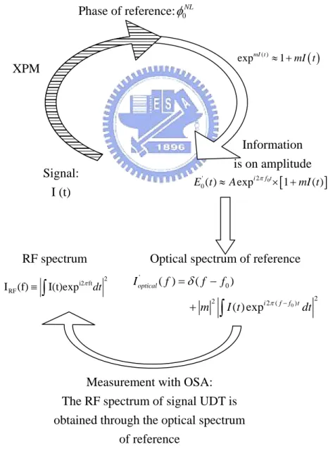
(22) Fortunately, these can be overcome or improved. To overcome the reduction from ‘m2’, we can choose a reference light with suitable power and resolve its optical spectrum after HNLF by an optical spectrum resolving devices with sufficient dynamic range as grating based OSA (optical spectrum analyzer) that has best dynamic performance in various types of OSA. [5] At the end of the section, let’s show the diagram to explain how the NLIFC accomplished, and the RF spectrum is copied to the optical spectrum of the reference light. Phase of reference: φ0NL expmI ( t ) ≈ 1 + mI ( t ). XPM. Information is on amplitude. Signal: I (t). E0' (t ) ≈ A expi 2π f 0t × [1 + mI (t ) ]. RF spectrum I RF (f) ≡ ∫ I(t)expi2π ft dt. Optical spectrum of reference 2. ' I optical ( f ) = δ ( f − f0 ). +m. 2. ∫ I (t ) exp. i 2π ( f − f 0 ) t. 2. dt. Measurement with OSA: The RF spectrum of signal UDT is obtained through the optical spectrum of reference Fig 1 Illustration of the working principle of optical RF spectrum analyzer 9.

(23) 2-2 Simulation of the optical spectrum of reference wave after NLIFC—. Estimate the maximum signal power without distorting the RF spectrum. In this section, the optical spectrum of the reference light passing through the HNLF is simulated with matlab according to the working principle of the optical RF spectrum analyzer described in section 2-1. The simulated result not only gives us a specific shape of the spectrum that we discussed but also helps us to do some prediction and discussion. For example, we can know the suitable signal power without distortion and see the difference between the optical spectrum of reference light after HNLF and the RF spectrum of signal that we want to measure.. “Illustration of the simulation”. The following picture shows the procedure of the simulation of the optical spectrum of the reference light passing through the HNLF. In the beginning, we create a time slot –‘t’ and generate the RZ ones train with supper Gaussian form: 2m ⎡ ⎛ 2 ( t − tD ) ⎞ ⎤ …eq. (2-10) y ( t ) = exp ⎢ −0.5 × ⎜ ⎟ ⎥ T ⎢⎣ ⎝ ⎠ ⎥⎦. , in which: (1) ‘ tD ’ adjusts the delay of the Gaussian pulse train. In our simulation, it is set as the half of the separation of each bit. For 10Gbps signal the bit separation is 0.1ns, so tD is chosen as 0.05ns. (2) ‘T’ is the width of each Gaussian pulse. (3) ‘m’ is the supper Gaussian factor. The larger the value of ‘m’, the shape of the pulse train is closer to a square wave. 10.

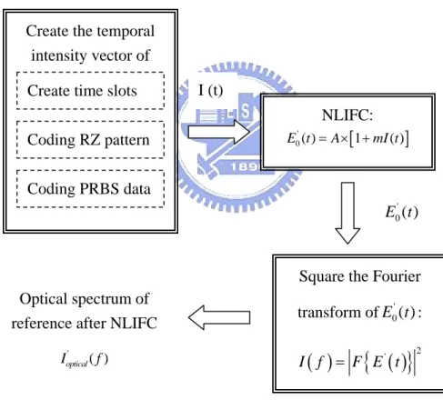
(24) Then use an n-bits “linear feedback shift register (LFSR)” to generate a PRBS (pseudo random binary sequence) with length of 2n-1 bits. Then calculate the E0' (t ) based on the eq. (2-8) but neglect the fast sinusoidal varying from expiω0t for reducing the load of computer. This approximation just leads the resulting spectrum to shift from the frequency of reference light, f0 to 0 and is not to matter much for us. Finally, after doing a Fourier transform and a square on E0' (t ) , we will obtain the ' optical spectrum of reference light after HNLF, Ioptical ( f ).. Create the temporal intensity vector of signal under test, I (t) Create time slots. I (t) NLIFC: E (t ) = A × [1 + mI (t ) ] ' 0. Coding RZ pattern Coding PRBS data. E0' (t ). Square the Fourier Optical spectrum of reference after NLIFC. transform of E0' (t ) : I ( f ) = F { E ' ( t )}. ' Ioptical (f). 2. Fig 2 Illustration oft the simulation of generation of optical spectrum of reference light after HNLF. 11.

(25) The simulation result. Following table describes the needed parameters that are according to practical experiment conditions. Sampling. Measurement Parameters. Fiber Properties. ti (initial time). tf (Stop time). slots interval. Length. Aeff. 0 ns. 100 ns. 0.01 ns. 1 km. 14.5 um2. γ. 1. / (km*W) 11.1. Signal light properties f. 10GHz. width. 0.03ns. Temporal. Gaussian. Average Power. PRBS length. bias. parameter. PI. 2^n-1. 0.05 ns. 1. 12.39/4.2mW. n=10. Reference light properties Power 0.5mW Table 1 Simulation parameters for 10Gbps signal. Note: 1. The effective area, Aeff=14.5um2 is determine by referring to the data sheet of Corning HNLF [Appendix C]. 2. The value of nonlinear coefficient,γis around 11.1. 1 that is estimated by Km ×W. observing the modulation instability (MI) gain spectrum of the HNLF. 3. The average power is according to the experiment condition. The signal power before entering the fiber 3-dB couple is around 14.7dBm, the loss of the coupler is 3.12dB and the connection loss between SMF and HNLF is 0.65dB. Thus the power entering the HNLF is 14.7-3.12-0.65=10.93dBm=12.39mW. 12.

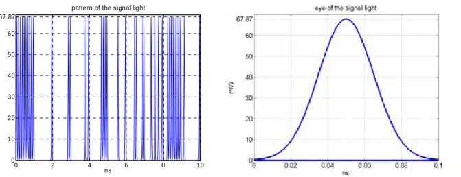
(26) 4. The simulated Eye diagram of signal matches that of experiment by adjusting the Gaussian parameter and the pulse width as the following diagrams: pattern of the signal light 67.87 60 50. mW. 40 30 20 10 0 0. 2. 4. ns. 6. 8. 10. Fig 3 Pattern and eye diagram of the simulated 10Gbps signal under test (Pav=12.39mW). 5. There is a relation between the amplitude of the signal (Pamp) and the average power of the signal (Pav): Pamp = Pav ×. max ( I ) × N …eq. (2-11) sum ( I ). , so Pav =67.87mW, when Pav=12.39mW. Then the following picture is the simulated resulting optical spectrum of the reference light passing through the HNLF. We can see the 10GHz harmonic peaks in the spectrum as our expectation. It is off course that we can’t measure an optical spectrum with so sharp peaks by general OSA, which has measurement resolution around 1GHz (0.01nm). The resolution of the spectrum in this simulation is assumed as the reciprocal of the duration of measurement (tf-ti), so in this case of tf-ti=100ns, the resolution of this spectrum is. 1 1 =0.01GHz. And, we take it as the real = t f − ti 100ns. spectrum before the distortion of the OSA measurement. We will also simulate the result after OSA measurement based on the spectrum in the next section, and it is. 13.

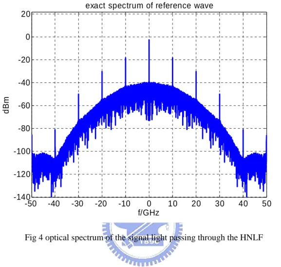
(27) more similar to the experiment result. exact spectrum of reference wave 20 0 -20. dBm. -40 -60 -80 -100 -120 -140 -50. -40. -30. -20. -10. 0 f/GHz. 10. 20. 30. 40. 50. Fig 4 optical spectrum of the signal light passing through the HNLF. Before doing that work, let’s show that the optical spectrum of the reference light after HNLF is almost the same with the RF spectrum of the signal light. Thus we simulate the RF spectrum of the signal under test according to the definition of RF spectrum—eq. (2-1) that is show in the figure 5. By comparing figure 4 and figure 5, we can find that the optical spectrum of the reference light is almost the same with the RF spectrum of the signal except that there is a down shift of figure 4 around 36.6dB that is originated from the square of ‘m’ in eq. (2-9) and an additional delta function causing a 8dB error in the center of figure 4.. 14.

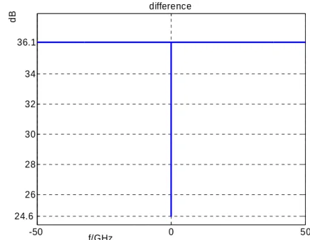
(28) RF spectrum of signal 20 0 -20. dBm. -40 -60 -80 -100 -120 -140 -50. -40. -30. -20. -10. 0 f/GHz. 10. 20. 30. 40. 50. Fig 5 RF spectrum of the signal under test. We can see these discussions in the following picture showing their difference. dB. difference. 36.1 34 32 30 28 26 24.6 -50. f/GHz. 0. Fig 6 Difference between RF spectrum signals and the optical spectrum of the reference light 15. 50.

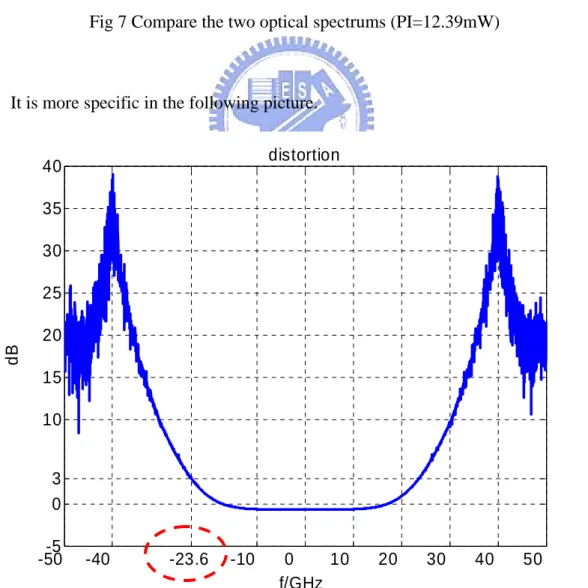
(29) Furthermore, the constant difference between the optical spectrum of the reference light and the RF spectrum of the signal shown in figure 6 proves that there is no distortion when we measure the RF spectrum of the signal by observing the optical spectrum of the reference light. All of these discussions can be justified in eq. (2-9). But it is needed to be declared that these conclusions are right based on the existence of the approximation: exp mI ( t ) ≈ 1 + mI ( t ) Following let’s to have some discussions about the influences of the key approximation. Distortion from the approximation— exp mI ( t ) ≈ 1 + mI ( t ). Although there is almost no distortion between the target RF spectrum of the signal (Fig 5) and the optical spectrum of the reference light calculated from eq. (2-8), the optical spectrum of the reference light calculated from eq. (2-8) is not the real one that be measured. In fact the optical spectrum of the reference light passing through the HNLF should be calculated based on the equation E0' (t ) = A expmI ( t ) . Following picture plots the optical spectrums of the reference light after HNLF in two cases: one is based on eq. (2-8) and another is based on E0' (t ) = A expmI ( t ) . We will find that there exists a specific difference between the two spectrums. Thus when we measure the RF spectrum of signal by observing the optical spectrum of the reference light, there will be a specific distortion that is originated from the approximation— exp mI ( t ) ≈ 1 + mI ( t ) and is the difference between the two spectrums in figure 7. In figure 7, we can also observe that the region without distortion is in the center of the spectrum with bandwidth around 20GHz (+20GHz~-20GHz). 16.

(30) the optical spectrum of reference 20 0. with exp(MI) with (1+MI). -20. dBm. -40 -60 -80 -100 -120 -140 -50. -40. -30. -20. -10. 0 f/GHz. 10. 20. 30. 40. 50. Fig 7 Compare the two optical spectrums (PI=12.39mW). It is more specific in the following picture. distortion. 40 35 30 25 dB. 20 15 10 3 0 -5 -50. -40. -23.6. -10. 0 10 f/GHz. 20. 30. 40. 50. Fig 8 distortion in the case of 10Gbps signal with 12.39 mW input power 17.

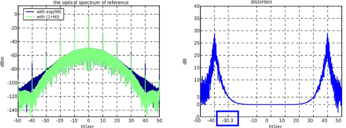
(31) It plots the difference between the two spectrums in dB scale in figure 8. We can see that the 3-dB bandwidth is only around 23.6 GHz ( ±23.9GHz ), so the correct measurement is restricted within the second harmonics for the 10Gbps signal, but fortunately the bandwidth can be increased by decreasing signal power, which can be predicted from the condition of the approximation— exp mI ( t ) ≈ 1 + mI ( t ) :. mI ( t ) << 1 Following picture shows the simulation corresponding to figure 7 and figure 8 in the case of PI=4.2mW that corresponds to the experiment with average signal power before entering 3-dB coupler around 10dBm. the optical spectrum of reference 0. 35. -20. 30. -40. 25. -60. 20 dB. dBm. distortion. 40. with exp(MI) with (1+MI). 15. -80. 10. -100 -120. 3 0. -140 -50. -40. -30. -20. -10. 0 f/GHz. 10. 20. 30. 40. -5 -50. 50. -40. -30.3. -10. 0. 10 f/GHz. 20. 30. 40. 50. Fig 9 the optical spectrums and distortion in the case of 10Gbps signal with PI=4.2mW. It is indeed that the region without distortion is broadened. Following picture is the relation between the signal power and the corresponding 3-dB bandwidth of region without distortion:. 18.

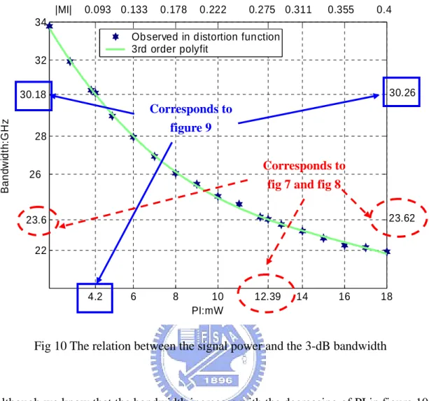
(32) |MI|. 0.093 0.133. 0.178. 0.222. 0.275 0.311. 0.355. 0.4. 34 Observed in distortion function 3rd order polyfit 32 30.26. Bandwidth:GHz. 30.18. Corresponds to figure 9. 28. Corresponds to fig 7 and fig 8. 26. 23.62. 23.6 22. 4.2. 6. 8. 10 PI:mW. 12.39. 14. 16. 18. Fig 10 The relation between the signal power and the 3-dB bandwidth. Although we know that the bandwidth increases with the decreasing of PI in figure 10, there is still a trade off in choosing the signal power, PI. Because the optical RF spectrum analyzer utilizes the nonlinear interaction in a HNLF—XPM, it is power sensitive and needs sufficient power to have obvious interaction. And, the OSA or other optical frequency resolving devices have a finite dynamic range or a finite noise floor, so the spectrum to be measured should be above the noise floor; otherwise the components under the noise floor will be buried. Thus we have to choose a suitable signal power to have widest range without distortion and above the noise floor of resolving devices. For example, if the noise floor is -80dBm, the PI=4.2mW (corresponding to Fig 9) is a better choice that has the bandwidth of the measurement range without distortion and above noise floor around 30 GHz for 10Gbps signal, so we can observe the complete and correct spectrum up 19.

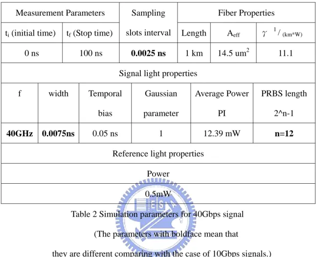
(33) to the third harmonic. As to the case of PI=12.39mW, the spectrum has distortion larger than 3dB outside ±23.6GHz , although it has larger range above -80dBm. But, if the noise floor is around -60dBm that is more reasonable for our practical experiment, although we can observe the peak of the third harmonic, some part between it and the peak of second harmonic is buried. However, a correct measurement range up to the second harmonic peak is guaranteed. These discussions will be justified later in the simulation involving the OSA measurement and practical experiment.. Simulation for 40Gbps signal. Now we have to think about an important problem: the region without distortion only has bandwidth around 20~35GHz that is discussed in the simulation for 10Gbps signal in last subsection, but what we want to design is an optical RF spectrum analyzer with ultra-wide bandwidth relative to conventional electrical RF spectrum analyzer that has very restricted bandwidth. Thus, the bandwidth caused by the distortion of the deviation of the key approximation almost destroys the plan. But, it is very fortunately that this kind of distortion has a special feature—the distortion depends on the RF signal under test itself. More specifically the bandwidth of region without distortion increases with the increasing of the repetition rate of the RF signal. It can be seen in the following simulation for 40Gbps signal. And the mathematical explanation is described in the next section. The setting parameters in the simulation program for 40Gbps signal are shown in the table 2. Most of them are the same with those for 10Gbps signal except “sampling slots interval”, “pulse width” and “the number of shifter register” (n). Because the bit rate is increased by 4 times, it is off course that the pulse width and the sampling slots interval should be quartered to maintain the same resolution of the resulting simulated 20.

(34) spectrum. And, the length of PRBS also should be increased by 4 times in the case without coding the PRBS twice. Measurement Parameters. Fiber Properties. Sampling. ti (initial time). tf (Stop time). slots interval. Length. Aeff. 0 ns. 100 ns. 0.0025 ns. 1 km. 14.5 um2. γ. 1. / (km*W) 11.1. Signal light properties f. 40GHz. width. 0.0075ns. Temporal. Gaussian. Average Power. PRBS length. bias. parameter. PI. 2^n-1. 0.05 ns. 1. 12.39 mW. n=12. Reference light properties Power 0.5mW Table 2 Simulation parameters for 40Gbps signal (The parameters with boldface mean that they are different comparing with the case of 10Gbps signals.). The results are shown in following pictures. pattern of the signal light. mW. 66.73. 0 0. 0.5. 1. 1.5. 2. 2.5. ns. Fig 11 Pattern and eye diagram of the 40Gbps signal under test (Pav=12.39mW). 21.

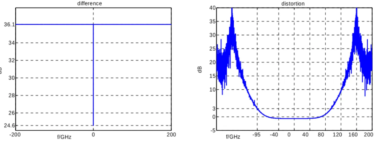
(35) the optical spectrum of reference. RF spectrum of signal. 20. 0. -20. -20. -40. -40 dBm. dBm. 0. 20 with exp(MI) with (1+MI). -60. -60. -80. -80. -100. -100. -120. -120 -140. -140 -200 -160 -120. -80. -40. 0 f/GHz. 40. 80. 120. 160. 200. -200 -160 -120. -80. -40. 0 f/GHz. 40. 80. 120. 160. 200. Fig 12 Resulting spectrums for 40Gbps signal with PI=12.39mW. difference. distortion. 40 35. 36.1. 30 34 25 32 dB. dB. 20 15. 30. 10 28 3 0. 26 24.6 -200. f/GHz. 0. -5. 200. f/GHz. -95. -40. 0. 40. 80. 120. 160. 200. Fig 13 Difference between the RF spectrum and optical spectrum and distortion caused by the key approximation for 40Gbps signal. From figure 11, we can see that the pulse shape of 40Gbps signal is almost with that of 10Gbps signal shown in figure 3, and figure 12 enable us to compare the RF spectrum of signal under test and the optical spectrums of reference light with and without the key approximation. We can find that the difference between RF spectrum and the optical spectrum of reference light in 40Gbps is the same with the case of 10GBps. Then let’s see the distortion caused by the deviation of the key approximation. It is shown by comparing the cases of 10G and 40G that the. 22.

(36) bandwidth of the region without distortion is increased by four times as the bit rate of signal under test. Thus the optical RF spectrum analyzer can also guarantee a correct measurement range up to the second harmonic peak for 40Gbps or higher bit rate signals at least. And, if the dynamic range of the OSA or other optical frequency resolving devices can have a little improvement, the correct measurement range can be broadened up to the third harmonic peak. As to the explanation of the lucky feature, we need to have a deeper understanding for the origin of distortion that will be discussed in next subsection.. Power expanding of Eo ( t ) = A exp −2π f0t expmI ( t ) '. ' In section 2-1, we obtain eq. (2-9)— I optical ( f ) = δ ( f − f 0 ) + m × ( I RF (f) ) f by the 2. 0. approximation: Eo ( t ) = A exp −2π f0t expmI ( t ) ≈ A exp −2π f0t ⎡⎣1 + mI ( t ) ⎤⎦ , but in fact there '. is still a lot of higher order terms neglected, which causes the distortion in the last subsection. In this subsection, we try to think about two questions: 1. Why does the distortion perform serious seriously in the edges of the spectrum? 2. Why does the region without distortion increase with the increasing of bit rate of signal under test? We still start from the electrical field of the reference light passing through HNLF. Eo ( t ) = A exp −2π f0t exp mI ( t ) '. = A exp. −2π f 0t. 2 3 ⎡ ⎤ mI ( t ) ) ( mI ( t ) ) ( ⎢1 + mI ( t ) + + + ...⎥ ≈ A exp −2π f0t ⎡⎣1 + mI ( t ) ⎤⎦ 2 6 ⎢⎣ ⎥⎦. If we calculate the optical spectrum with the last equation as the produce in the last section, we will have: 23.

(37) ' I optical (f)=. ' i 2π ft ∫ E0 (t ) exp dt. 2. 2 ⎛ ⎡ ⎤⎞ mI ( t ) ) ( − i 2π f 0 t 2 ⎜ = A ∫ exp × ⎢1 + mI (t ) + + ...⎥ ⎟ expi 2π ft dt 2 ⎜ ⎢⎣ ⎥⎦ ⎟ ⎝ ⎠ 2 ⎡ ⎤ mI ( t ) ) ( 2 = A ∫ ⎢1 + mI (t ) + + ...⎥ expi 2π ( f − f0 ) t dt 2 ⎢⎣ ⎥⎦. 2. 2. ⎛ ( mI ( t ) )2 ⎞ i 2π ( f − f 0 ) t i 2π ( f − f 0 ) t 2 ⎟ expi 2π ( f − f0 ) t dt + ... = A ∫ exp dt + ∫ ( mI (t ) ) exp dt + ∫ ⎜ ⎜ ⎟ 2 ⎝ ⎠ If we only consider the first three terms and expand the last equation: ' I optical (f). ⎛ ( mI ( t ) )2 ⎞ i 2π ( f − f 0 ) t i 2π ( f − f 0 ) t 2 ⎟ expi 2π ( f − f0 ) t dt dt + ∫ ( mI (t ) ) exp dt + ∫ ⎜ = A ∫ exp ⎜ ⎟ 2 ⎝ ⎠. 2. ⎡ ⎤ ⎛ ( mI ( t ) )2 ⎞ i 2π ( f − f 0 ) t i 2π ( f − f 0 ) t ⎢ ⎟ expi 2π ( f − f0 ) t dt ⎥ dt + ∫ ( mI (t ) ) exp dt + ∫ ⎜ = A ∫ exp ⎜ ⎟ 2 ⎢ ⎥ ⎝ ⎠ ⎣ ⎦ 2. ⎡ ⎤ ⎛ ( mI ( t ) )2 ⎞ i 2π ( f − f 0 ) t i 2π ( f − f 0 ) t ⎢ ⎟ expi 2π ( f − f0 ) t dt ⎥ × ∫ exp dt + ∫ ( mI (t ) ) exp dt + ∫ ⎜ ⎜ ⎟ 2 ⎢ ⎥ ⎝ ⎠ ⎣ ⎦. *. ⎡ ⎤ ⎛ ( mI ( t ) )2 ⎞ i 2π ( f − f 0 ) t ⎟ expi 2π ( f − f0 ) t dt ⎥ dt + ∫ ⎜ = A ⎢δ ( f − f 0 ) + ∫ ( mI (t ) ) exp ⎜ ⎟ 2 ⎢ ⎥ ⎝ ⎠ ⎣ ⎦ 2. ⎡ × ⎢δ ( f − f 0 ) + ⎢ ⎢⎣. (. ⎛ ⎛ ( mI ( t ) )2 ⎞ ⎞ i 2π ( f − f 0 ) t i 2π ( f − f 0 ) t ⎜ ⎜ ⎟ ⎟ ( ) exp exp mI t dt dt + ( ) ∫ ⎟ 2 ⎜∫⎜ ⎟ ⎠ ⎝ ⎝ ⎠. ). *. *. ⎤ ⎥ ⎥ ⎥⎦. Follow the derivation in section 2-1, we have: ' I optical (f). ⎡ ⎤ ⎛ ( mI ( t ) )2 ⎞ i 2π ( f − f 0 ) t i 2π ( f − f 0 ) t ⎢ ⎜ ⎟ dt + ∫ dt ⎥ ∝ δ ( f − f 0 ) + ∫ ( mI (t ) ) exp exp ⎜ ⎟ 2 ⎢ ⎥ ⎝ ⎠ ⎣ ⎦ ⎡ ⎢ × δ ( f − f0 ) + ⎢ ⎣⎢. (. ⎛ ⎛ ( mI ( t ) )2 ⎞ ⎞ i 2π ( f − f 0 ) t i 2π ( f − f 0 ) t ⎜ ⎟ ⎜ ⎟ mI t dt dt ( ) exp exp + ) ∫( ⎟ 2 ⎜∫⎜ ⎟ ⎠ ⎝ ⎝ ⎠. ). 24. *. *. ⎤ ⎥ ⎥ ⎦⎥. 2.

(38) ' I optical (f). ∝ δ ( f − f0 ) +. ∫ ( mI (t ) ) exp. i 2π ( f − f 0 ) t. 2. dt. ⎛ ⎛ ( mI ( t ) )2 ⎞ ⎞ i 2π ( f − f 0 ) t ⎟ expi 2π ( f − f0 ) t dt ⎟ dt × ⎜ ∫ ⎜ + ∫ ( mI (t ) ) exp ⎟ 2 ⎜ ⎜ ⎟ ⎠ ⎝ ⎝ ⎠. (. *. ). ⎛ ⎛ ( mI ( t ) )2 ⎞ ⎞ ⎟ expi 2π ( f − f0 ) t dt ⎟ × +⎜∫⎜ ⎟ 2 ⎜ ⎜ ⎟ ⎠ ⎝ ⎝ ⎠ ⎛ ( mI ( t ) )2 ⎞ ⎟ expi 2π ( f − f0 ) t dt + ∫⎜ ⎜ ⎟ 2 ⎝ ⎠. ( ∫ ( mI (t )) exp. i 2π ( f − f 0 ) t. ). *. dt +. 2. 2. = δ ( f − f0 ) +. ∫ ( mI (t ) ) exp = m I RF (f) 2. i 2π ( f − f 0 ) t. 2. dt. ⎛ ( mI ( t ) )2 ⎞ ⎟ expi 2π ( f − f0 ) t dt ...eq.(2 − 12) + ∫⎜ ⎜ ⎟ 2 ⎝ ⎠. (term1). error. (term 2). Compare eq. (2-12) with eq. (2-9). And, we can find that the additional error term is appeared. And, the previous two questions can be answered from the error term. Following picture compare term1 and term2 in eq. (2-12). spectrum of term1 and term2 -11.21 -16.67. dBm. -40. -60. -80 Spectrum of MI Spectrum of (MI)2 / 2. -100 -50. -40. -30. -20. -10. 0. 10. 20. 30. f/GHz. Fig 14 Spectrums of term1 and term2 in eq.2-12 25. 40. 50.

(39) In the figure 14, we find that the spectrum of. ( MI ) 2. 2. (the term 2) has larger high. frequency components than that of (MI) (the term 1), which is due to the operation of. ( MI ) square. And, the spectrum of 6. 3. ,. ( MI ) 24. 4. and other higher order terms will have. larger components in high frequency, but there higher order terms are all neglected in eq. (2-8) and eq. (2-9), so it is obvious that there are larger distortion in the edge. As to the question2, because the distortion originates from the higher order terms of signal under test, it is off course that the region without distortion will broaden with the broadening of the spectrum of signal under test or the narrowing of its pulse width. In the simulation, the pulse width is decreased in the same ration when the bit rate increase from 10Gbps to 40Gnps. Thus the region without distortion also broadens by 4 times.. 26.

(40) Chapter Three. Setup of the optical RF spectrum analyzer. 3-1 Required highly nonlinear fiber (HNLF). The key of the optical RF spectrum analyzer is the highly nonlinear fiber that performs the XPM between the signal light and reference light. Although there is still other component able to perform the XPM between two lights, for example— SOA (semiconductor optical amplifier) that is popular in the application of wavelength conversion, the HNLF is still the better choice in this application—constructing the high bandwidth optical RF spectrum analyzer. It is because that the applied nonlinear interaction in HNLF has much larger bandwidth—10THz [3]. Thus, we also choose the HNLF in our experiment. Following is the data sheet of the Corning C-band highly nonlinear fiber that we use. It is obtained from Corning. Item. Specification. Unit. Operating Wavelength. 1550. nm. Attenuation @ 1550 nm. ~ 0.5. dB/km. Attenuation @ 1380 nm. ~2. dB/km. Cutoff. ~1150. nm. Effective Area. 14-15. µm^2. Zero Dispersion Wavelength. 1550 +/- 20. nm. Dispersion Slope @ 1550 nm. ~0.04. ps/nm^2/km. Table 3 Corning Highly Non-linear, Zero Dispersion @ 1550 Specialty Fiber. 27.

(41) Item. Specification. Unit. Dispersion @ 1525 nm. ~ -1.0 to -1.7. ps/nm^2/km. Dispersion @ 1550 nm. - 0.08 to -0.6. ps/nm^2/km. Dispersion @ 1575 nm. 0.98 to 0.31. ps/nm^2/km. Cladding Outside Diameter. 125 +/- 2. µm. Coating Outside Diameter. 245 +/- 15. µm. Coating. Dual UV-curable acrylate. Table 3 Corning Highly Non-linear, Zero Dispersion @ 1550 Specialty Fiber (continued). But, the data sheet is not detailed enough for us. We still need the nonlinear coefficient,γand the dispersion properties of the HNLF. Thus we do some simple measurements to know it more that are described in following paragraphs.. 3-1-1: The measurement of its high nonlinear coefficient. We have assumed the nonlinear coefficient, γ around 11.1 1. ( km × W ). in the. previous simulation in section 2-2. It is the result of estimation in the following experiment— observation of the MI (modulation instability) gain spectrum of a light passing through the HNLF. There are several different approaches for measuring the nonlinear coefficient [6], which are classified by two types: interferometric methods and non-interferometric methods. What we adopt is based on the modulation instability that belongs to the non-interferometric methods, because of its simplicity. [7][8] Before entering the measurement of nonlinear coefficient by modulation 28.

(42) instability, we have a brief introduction about the phenomenon—modulation instability. [4]. Generation of modulation instability— Linear stability analysis of nonlinear Schrodinger equation. Modulation instability originates from the interplay between nonlinear and dispersive effects. It only occurs in the anomalous dispersive region (D>0 or ß2<0). These can be explained from the “linear stability analysis of nonlinear Schrodinger equation” stated as below. Equation (3-1) is the nonlinear Schrodinger equation neglecting the loss term. i. ∂A 1 ∂ 2 A 2 = β 2 2 − γ A A …eq. (3-1) ∂z 2 ∂T. , where A (z, T) is the amplitude of the pulse envelope, β 2 is the GVD parameter and γ is the nonlinear coefficient. In the case of CW, radiation at the input end of the fiber, i.e. A ( 0, T ) = constant: If there is no any noise or perturbation inside the fiber in the propagation process, we will have a steady-state solution by assuming that the A is independent of time (, so solve the equation: i. 2 ∂A = −γ A A ): ∂z. A = P0 eiΦ NL , Φ NL = γ P0 z This solution means that the amplitude of incident light is unchanged except acquiring a power-dependent phase shift. But, there is always some noise or perturbation in the fiber, so let’s discuss weather the steady-state solution is stable for a small perturbation: Let’s assume. 29.

(43) A ( z, T ) =. (. ). P0 + a ( z, T ) eiΦ NL …eq. (3-2). Substitute eq. (3-2) into eq. (3-1), then we have: i. ∂a 1 ∂2a = β 2 2 − γ P0 ( a + a* ) …eq. (3-3) ∂z 2 ∂T. If we assume a general solution of the form: a ( z , T ) = a1 cos ( Kz − ΩT ) + ia2 sin ( Kz − ΩT ) …eq. (3-4). , the eq. (3-3) will provide a set of two equations for a1 and a2. And, from the representation of a1 and a2, we will obtain the relation between the K andΩ: K =±. 1/ 2 1 β 2 Ω ⎡⎣Ω 2 + sgn ( β 2 ) Ω c 2 ⎤⎦ …eq. (3-5) 2 4γ P0 2 Ωc = …eq. (3-6). β2. (Derivation) With eq. (3-3): i. ∂a 1 ∂2a = β 2 2 − γ P0 ( a + a* ) ∂z 2 ∂T. Because a ( z , T ) = a1 cos ( Kz − ΩT ) + ia2 sin ( Kz − ΩT ) ∂a = − a1 K sin ( Kz − ΩT ) + ia2 K cos ( Kz − ΩT ) ∂z ∂ 2a = − a1Ω 2 cos ( Kz − ΩT ) − ia2Ω 2 sin ( Kz − ΩT ) , ∂z 2 a + a* = 2a1 cos ( Kz − ΩT ). Thus, we have the following two equations: a2 K =. β 2 a1Ω 2. 2 β a Ω2 a1 K = 2 2 2. β 2 2Ω4 +. + 2γ a1 P0. K2 =. K2 =. β 2 2Ω 4 4. 2K. ⎛ β 2 a2 Ω 2 ⎞ ⎟ + 2γ P0 ⎜ 2 K ⎟ ⎠ ⎝ ⎠. + γβ 2Ω 2 P0 =. 2. 4 1/ 2. ⎡ ⎛ 4γ P0 ⎞ ⎤ Ω ⎢Ω 2 + sgn( β 2 ) ⎜⎜ K =± ⎟⎟ ⎥ 2 ⎝ β 2 ⎠ ⎦⎥ ⎣⎢. β 2 Ω 2 ⎛ β 2 a2 Ω 2 ⎞ 2 ⎜⎝. β2. 4γβ 2 Ω 2 P0. β2. Then, we can eliminate the a1: a2 K =. sgn( β 2 ). K =±. β 2 2Ω4 + 4γβ 2Ω2 P0 4. β2. 1/ 2. 2 Ω ⎡⎣Ω 2 + sgn( β 2 )ΩC ⎤⎦ , 2 4γ P0 2 where Ωc =. β2. 30.

(44) The eq. (3-5) shows that the stability of the steady-state depends on weather light experiences normal or anomalous dispersion. In the case of normal dispersion (D<0, ß2>0), the K is always real for all Ω , so the steady state is stable for small perturbation. But, in the case of anomalous dispersion (D>0, ß2<0), the K is imaginary for Ω<Ωc, so the perturbation will grows exponentially with z and the steady state solution is unstable, so a MI gain spectrum exists around the input laser that can be calculated by eq. (3-5). Thus there are side lobes in the optical spectrum of the laser after MI interaction, and the CW input laser is broken into a train of ultra-short pulses.. MI gain spectrum. Because our measurement of the nonlinear coefficient utilizes the observation of the MI gain spectrum, we discuss the relation between the MI gain coefficient and the nonlinear coefficient that we want to measure here. Besides the nonlinear coefficient, the experiment can also give us the dispersion parameter, D and zero dispersion wavelength,λ0. When the pump laser is operated at anomalous GVD and Ω < Ωc , the perturbation will growth exponentially with z, so we will have a gain spectrum in ω0 ± Ω . a ( z ) ~ e jKz = e a ( z) = e 2. Substitute the equation K = ±. i Re{ K } z − Im{ K } z. e. −2Im{ K } z. =e. g (Ω) z. ,. 1/ 2 1 β 2 Ω ⎡⎣Ω 2 + sgn ( β 2 ) Ω c 2 ⎤⎦ , and then we have: 2. (. g ( Ω ) = −2 Im { K } = β 2 Ω Ω c − Ω 2. Ω max =. ,. 2. ). 1/ 2. …eq. (3-7). Ωc 1 2 ; g max = β 2 Ωc …eq. (3-8) 2 2. , where g is the gain coefficient in unit of 1/km. 31.

(45) The eq. (3-7) and eq. (3-8) are the simple mathematically describing for the MI gain spectrum. Then let’s rewrite them by some physical parameters with the relation— Ωc = 2. 4γ P0. β2. : 1/ 2. ⎛ 4γ P0 ⎞ − Ω 2 ⎟⎟ g ( Ω ) = β 2 Ω ⎜⎜ ⎝ β2 ⎠. …eq. (3-9). 1/ 2. Ω max. ⎛ 2γ P0 ⎞ = ⎜⎜ ⎟⎟ ; g max = 2γ P0 …eq. (3-10) β 2 ⎝ ⎠. The following figures show the simulated MI gain coefficient and gain spectrum corresponding to the experiment with 1559nm input laser. The needed parameters are set as: β 2 = −0.38 ps 2 / km , γ = 11.1. 1 , input power=16dBm(around 0.0398W) W • km. and fiber length=1Km. MI gain coefficient. MI gain coefficient,g:1/km. 0.884. 0.6. 0.4. 0.2. Wavelength shift: nm. 0. 0.405 0.05. 0.81 1.215 1.944 2.43 0.1 0.15 0.243 0.3 frequency shift:THz. Fig. 15 simulated MI gain coefficient (input laser with power=16dBm, λ=1559nm). 32.

(46) MI gain spectrum 3.838. MI gain spectrum, G:dB. 3. 2. 1. 0. 0.405 0.05. Wavelength shift: nm 0.81 1.215 1.944 2.43 0.1 0.15 0.243 0.3 frequency shift:THz. Fig. 16 simulated MI gain spectrum (input laser with power=16dBm, λ=1559nm). Observation of MI gain spectrum. Before explaining how to estimateγ, D and λ0 from the MI gain spectrum, lets explain the experiment setup and the observed MI gain spectrum first. The experiment setup for observing the MI gain spectrum is very simple and shown in the following figure. HNLF Tunable Laser. EDFA. OSA. Fig 17 Experiment setup of the observation of the MI gain spectrum 33.

(47) We measure the MI gain spectrum produced by our HNLF in various input powers and wavelengths. Following figure shows one of these results that the input power is around 16dBm and its wavelength is at 1559nm. laser spectrum at 16dBm 1559nm pump 15.5. 11.94. power:dBm. without passing through CHNLF with passing through CHNLF. -20 -40 1545. 1559 1565 wavelength:nm gain spectrum at 16dBm 1559nm pump. 3.57. 1575. gain:dB. 3.36. 3.3. 3.48. 0 1559 1562.48 wavelength:nm 1555.7. Fig 18 MI gain spectrum (PI=16dBm,λ=1559nm). In the figure16 and figure 18, we notice two important indexes—the max value of the MI gain spectrum, Gmax and the frequency shift, Δf , in which the max gain occurs ( ∆f =. Ω max. 2π. ). The measured value of Gmax is close to that in the simulation,. but the measured value of Δf has larger difference with that in the simulation. I think it is because that value of γ(=11.1. 1. ( km × W ). ) is determined by this experiment. but that of ß2 is by the measurement of an optical network analyzer. From eq. (3-11) we can know that Gmax ( = exp( g max L) ) is determined by γ, but. 34.

(48) 1/ 2. Ω max. ⎛ 2γ P0 ⎞ = ⎜⎜ ⎟⎟ is inverse proportional to ( β 2 β 2 ⎝ ⎠. ). 1/ 2. , which can be justified by the. comparison between the experimental and simulated results.. Estimation of γ, ß2 (D) and λ0. From the eq. 3-10, we can know that the maximum gain coefficient, gmax and the square of the frequency shift, Δf. 2. are proportional to the input laser power, so we. can have the following results and use the slopes— m( gmax ,P0 ) and m( ( ∆f )2 ,P ) to 0. estimate γ, ß2 and λ0. m( gmax ,P0 ) is the slope of the relation between gmax and input laser power, and m( f. 2 max. , P0 ). is that between Δf and input laser power.. (1) Calculate the nonlinear coefficient, γ. g max = 2γ P0 , g max = m( gmax , P0 ) , P0. γ=. m( gmax , P0 ). …eq. (3-11). 2. (2) Calculate the absolute value of ß2. ⎛ 2 γ P0 ⎞ 2π × ∆ f = ⎜ ⎟ ⎝ β2 ⎠. ( 4π ) 2. (∆f ) × P0. m( ( ∆f )2 , P ) 0. 35. 1/2. 2. =. …eq. (3-12) 2γ. β2. ( ∆f ) = P0. 2.

(49) β2 =. 2γ ( 4π ) × m((∆f )2 ,P ) …eq. (3-13) 2. 0. Following picture shows the MI gain spectrum measured at input laser at various conditions.. gain spectrums at 1553nm pump. gain spectrums at 1556nm pump. gain:dB. gain:dB. gain:dB. 3 3 2.5 2.5 2 2 1.5 1.5 1 1 0.5 0.5 0 0 -0.5 -0.5 -1 -1 1535 1545 1555 1565 1540 1550 1560 1570 wavelength:nm wavelength:nm gain spectrums at 1559nm pump 3.5 3 2.5 pump at 14dBm 2 pump at 15dBm 1.5 pump at 16dBm 1 The measurment span=20nm 0.5 0 centered at the laser wavelength -0.5 -1 1540 1550 1560 1570 wavelength:nm Fig 19 The MI gain spectrums. There are some things that can be found in figure 19: 1. The shorter the laser wavelength, the larger the span of MI gain spectrum. It is because that the absolute value of ß2 is smaller in shorter wavelengths after λ0. And it can be explained by eq. (3-12). 2. The MI gain spectrum corresponding to the laser wavelength at 1553nm is different with the MI gain spectrum corresponding to the laser wavelengths at. 36.

(50) 1556nm and 1559nm—the gain peak at longer wavelength is higher than that at shorter wavelength. And, we will see the following results corresponding to 1553nm laser wavelength have larger deviation. It should be because the MI occurs in the anomalous dispersive region and the λ0 of our HNLF is in 1552nm. Then, the following figure shows the linear relation between gmax and PI and that between Δf 2 and PI.. 0.9. 1.4. 0.8. max gain coefficient:1/km. 0.7 0.6 0.5 0.4 0.3 0.2 0.1 0. pump pump pump pump pump pump. at at at at at at. 1553 1553 with linear fit 1556 1556 with linear fit 1559 1559 with linear fit. square of shift frequency:THz2. 1.2. pump pump pump pump pump pump. at at at at at at. 1553 1553 with linear fit 1556 1556 with linear fit 1559 1559 with linear fit. 1. Extreme estimation: 0.8 m ~40 B 0.6. Our fitting: mG~26. 0.4 0.2 0. -0.1 0 0.010.020.030.040.05 pump power:W. -0.2 0. 0.01 0.02 0.03 0.04 0.05 pump power:W. Fig 20 Left: The linear relation between gmax and PI Right: The linear relation between Δf 2 and PI. In figure 20, the dots are measured data and the lines are linear fittings. We can obtain the slopes that we desired from the fitting lines. We can utilize the slopes of the three fitting lines in the left figure to calculate the γ corresponding to the three wavelengths. And, the absolute values of ß2 at the three. wavelengths are obtained by the slopes of the three lines in the right figures. 37.

(51) Furthermore, we know the sign of ß2 are negative, because the MI occurs only in the anomalous dispersive region. Then we can derive D from ß2 with the following. D:ps/km*nm. abs(bata):ps 2 /km rmax:1/W*km. equation— D =. −2π c. λ2. β 2 . These are show in the following figure.. 11.19. 10.93. 9.22 1553. 1556. 1559. 1553. 1556. 1559. 0.1457 0.0728 0.0162. 0.113 0.0567 0. D-Slope=0.0167 ps/km nm2 ╳. 0.0127 1553. wavelength:nm λ0=1552.37 nm. 1556. 1559. Fig 21 The values of γ, │ß2│ (D) and λ0. Finally, λ0 is obtained by stretching the fitting line of the D to the intersection point with zero. We can obtain some conclusions and have some discussions in figure 20 and figure 21: 1. The value of γ of this HNLF is around 11.1 1. km × W. , which is obtained by. averaging the value of γ measured in 1556 nm and 1559 nm. We neglect the value at 1553 nm, because we think that it is incorrect. 2. The value of γ shown in figure 21 is not direct calculated from eq. (3-11), 38.

(52) because the calculation directly from eq. (3-11) and the measured slope of the relation between gmax and PI actually refers to random polarization. That referring to linear polarization and marked in the figure 21 needs an additional transforming factor— 9. 8. . [8] Besides that, we need to modify the reduction of the fiber loss.. [4] Thus the value of γ marked in figure 21 is calculate by following equation.. γ=. m( gmax ,P0 ) 2. 9 × × ( Loss ) −1 …eq. (3-14) 8. And, the equation (3-15) is also modified as:. β2 =. ( 4π ) × m (. 2γ. × ( Loss ) ( ∆f ) , P ). 2. −1. …eq. (3-15). 2. 0. , so we know that the absolute value of ß2 is independent with the fiber loss. 3. Note the right figure in Fig. 20. There are a large difference between the measured data (dots) and the fitting line, which is because we force Δf (PI=0) = 0 that is according to eq. (3-12); or the slope will be greatly underestimated, and│ß2│and D will be overestimated. 4. Following discussion is the error of m( ( ∆f )2 ,P ) and the resulting error of │ß2│at 0. 1553 nm laser wavelength. In the right figure of Fig.20, we seem to underestimate m( ( ∆f )2 ,P ) │1553nm , but we will show that its influence is very limited in following 0. results—│ß2│at 1553 nm and λ0. In our measurement, the maximum m( ( ∆f )2 ,P ) 0. at 1553 nm is around 40 THz. 2. W. belonging to the black line.. Then we assume the relative error of m( ( ∆f )2 ,P ) │1553nm as: 0. Error m. ( ( ∆f )2 , P0 ). =. mG − mB 26 − 40 = = −53.8% …eq. (3-16) mG 26. , and that of │ß2│ at 1553 nm as:. 39.

(53) Error. β 2 ,1553nm. =. β2 G − β2 B …eq. (3-17) β2 G. And, with eq. (3-15), we can express eq. (3-17) as mG and mB.. Error. β 2 ,1553 nm. =. β2 G − β2 B β2 G. =. mB − mG mB. =. 40 − 26 = 35% 40. ;. Furthermore, we know that the relative error of D equals to that of │ß2│from the relation between D and ß2.. Error D ,1553nm =. DG − DB = 35% DG. Thus the difference between │ß2│G and │ß2│B (or DG and DB) at 1553nm is very small, because it is nearλ0 of the fiber.. ∆. β2. = β2 G − β2 B. ∆ D = DG − DB. = β 2 G × Error 2 = 0.0162 ps 2 = 0.0057 ps. β 2 ,1553nm. km. × 35%. km. = DG × Error D ,1553nm = 0.0127 ps. 2. = 0.0044 ps. 2. km. × 35%. km. So the measurement of ß2 and D has nice linear dependence and well prediction of λ0=1552.37 nm.. 3-1-2: The measurement of its dispersion properties. Although the MI gain spectrum also tells us the dispersion properties of HNLF, we also make a more detailed measurement of the dispersion properties of the HNLF with the ADVANTEST Q7760 optical network analyzer. The obtained result not only 40.

(54) gives us a comparison with that obtained by MI gain spectrum but also lets us able to do the prediction of the bandwidth of our optical RF spectrum analyzer based on the. 15 9. D:ps/nm.km. 3 -0.0386. Dslope:ps/nm 2 .km. measured 0.99-rloess smooth 2nd poly fit. 1530. 1540. 1552.04 1560. 2 0.0051 -2. 1570. 1580. measured 0.99-rloess smooth derived by the fit of GD. 1530. 1540. 1552.04 1560. 1570. 1580. measured 0.99-rloess smooth derived by the fit of GD. 2 0.0418 -2. 1530 1535 1540 1545 1550 1555 1560 1565 1570 1575 1580 wavelength:nm. 0.2959. measured 0.99-rloess smooth derived by the fit of GD. D:ps/nm.km. relative GD:ps. measured dispersion data in chapter 4.. 0.1706. 0.0452. 1553 1556 wavelength:nm. 1559. Fig 22 Dispersion properties of Corning HNLF measured by ADVANTEST Q7760 optical network analyzer 41.

(55) In figure 22, the blue dots are the initial measured data from Q7760 and the green solid lines are that after smoothing. Furthermore, we also use the 2nd order polynomial fitting to describe the relative GD (group delay)—the coffee dot line in first figure, and we can obtain the function describing D (dispersion) and D-slope utilizing the 2nd order polynomial GD by differentiation—the coffee dot line in second and third figures. For the completeness, we calculate relative ß1 and ß2 utilizing the fitting function. bata2:ps2 /km. relative bata1 :ps/km. of D in figure 22.. 15 obtained by integration the Dispersion versus landa. 9 3 0. 1530. 1540. 1552.04 1560 wavelength:nm. 1. 1570. 1580. 2. obtained by bata2=(-(landa)/(2piC))D. 0.0033 -0.38 -1 1530. 1540. 1551.861559 wavelength:nm. 1570. Fig 23 dispersion properties of Corning HNLF. The relative ß1 and ß2 are calculated by following equations.. d β1 dλ −2π c. D= D=. λ2. β2. ∴∆β1 = ∫ β1d λ …eq. (3-18) ∴ β2 = − 42. λ2 D …eq. (3-19) 2π c. 1580.

(56) In following table, we have a simple compression about some parameters from the measurement of MI gain spectrum and Q7760.. D. ß2. Parameters. MI. Q7760. λ0. 1552.37 nm. 1552.04 nm. D-slope. 0.0167 ps/km nm2. 0.0418 ps/km nm2. 1553 nm. 0.0127 ps/km nm. 0.0452 ps/km nm. 1556 nm. 0.0567 ps/km nm. 0.1706 ps/km nm. 1559 nm. 0.113 ps/km nm. 0.2959 ps/km nm. 1553 nm. -0.0162 ps2/km. -0.0579 ps2/km. 1556 nm. -0.0728 ps2/km. -0.2191 ps2/km. 1559 nm. -0.1457 ps2/km. -0.38 ps2/km. ╳. ╳. ╳. ╳. ╳. ╳. ╳. ╳. Table 4 Compression of measured results from MI gain spectrum and Q7760. Although there are some differences existing between the values obtained from these two approaches, the trends and orders still agree with each other.. 3-1-3: Control and estimate the loss. Reduction the fusion loss between HNLF and SMF. The HNLF has a much smaller core than general SMF, so there is a larger splicing loss when they are fused together. But, we can reduce the spicing loss through adjusting the fusion parameters including the discharging duration, discharging intensity and push moment. The fiber is fused by the fiber splicer— “Sumitomo Electric type 36”. The best fusion condition is described in the following table and. 43.

(57) saved in “Sumitomo Electric type 36”. Parameters. Best setting. Standard(SMF). Units. Discharging duration. 13. 1.05. second. Discharging intensity. 17. 9. step. Push moment. 10. 15. um. Table 5 The best fusion conditions of for fusing the HNLF and SMF. At this condition the splicing loss is around 0.6~0.7 dB.. Estimate the splicing loss and the intrinsic loss of HNLF. TL. Power Meter. SMF28. Measure the Reference Power1 Bare fiber Connector Fusion Point. Power Meter. TL. HNLF (1km) Splicing Loss in Er-other2 mode, L1=L (HNLF) +L (splice, 1) =1.1 dB. TL. Fusion Point. Fusion Point. Power Meter. L2=L (HNLF) +L (splice,1)+L(splice,2)-V=1.5 dB Fig 24 Setup of measuring the intrinsic loss of HNLF and splicing loss. 44.

(58) In figure 24, ‘V’ is the loss decreasing caused by instating the bare fiber connector with a PC connector and is measured as 0.25dB in previous experiment. With ‘V’, ‘L1’ and ‘L2’, we can estimate the intrinsic loss of HNLF and the splicing loss: L (HNLF) = 0.45 dB L (splice, 1) = L (splice, 2) =0.65 dB , which agree with the previous data.. 45.

(59) 3-2 Measurement results of 10Gbps and 40Gbps signal. In this section, our optical RF spectrum analyzer will be shown. Following figure is a sketch of the optical RF spectrum analyzer. It is so simple that we need only a HNLF and an OSA to measure the RF spectrum of the signal under test. Signal under test. Coupler 50/50 OSA. E0' (t ) Tunable Laser. Fig 25 A sketch of the optical RF spectrum analyzer. And, for demonstrating its high bandwidth performance, we use it to measure the RF spectrum of two signals: one is 10GBps RZ signal with/without coding (210-1) PRBS; the other is 40GBps RZ ones train.. 3-2-1: 10GBps signal. In this subsection, the measurement of RF spectrum of 10GBps signals by this new all optical approach is demonstrated. The following picture is the detailed experiment setup and the table describes the experimental conditions. 46.

(60) Experiment setup and conditions. Generation of signal under test. Pattern Generator. Driver RF Amp.. 10G Synthesizer (-4.5dBm). PC DFB. EA. IM. DL. A. TL. EDFA B Filter. Attenuator Coupler 50/50. Control the signal power. HNLF 1km OSA ADVENTEST Q8384. NLIFC Observation. Fig 26 Experimental setup of the RF spectrum of 10Gbps signal 47.

(61) Physical condition RZ train coding IF. TC 84.8mA 16.7℃. PRBS coding. TL. EABIAS. RF power. VBIAS. VGC. Power. λ. -1.22V. -4.5dBm. +1.22V. -6V. 3.5dBm. 1554nm. Measurement Instrument OSA. Sampling Scope. Resolution. Sampling points. Scale. Offset. 0.01nm. 1001. 500uW/div. 300uW. Table 6 experimental conditions for 10Gbps signal. In figure 26, the thick lines represent the path of electrical RF signal (RF cable); and thin lines represent that of optical signal (fiber). The setup is divided into four parts: generation of signal under test, controlling the signal power, NLIFC and observation, which are all marked in the figure 26. First we have to generate an optical signal under test. In this part, we choose to generate a 10GBps RZ signal. The 10GHz sinusoidal signal is generated from the “Agilent 83624B signal generator”. It is split into two parts: one is used to trigger. the “Anritsu pulse pattern generator” that generates a PRBS data and the other enters the “Agilent 83017A microwave system amplifier”. The amplified 10GHz sinusoidal signal is sent into the EA (electrical absorption) modulator, and the continuous light from DFB laser is modulated as a RZ ones train. Then the optical RZ ones train passes through a DL (delay line) that is used to synchronize the RZ ones train and the PRBS coding. The PRBS coding is performed by the “JDSU 10GBps Lithium Niobate AM modulator” and the “Picosecond Pulse Lab model 5865 modulator driver”. Now the optical signal under test as that. in figure 3 is generated. We observe it at ‘A’ with Agilent sampling scope. The result is shown in figure 27. 48.

(62) Then the optical signal is amplified by an EDFA and an optical filter that suppress the ASE from EDFA. Following the filter we insert an optical attenuator to adjust the power of the signal under test. We also utilize the sampling scope to see the eye of the signal under test after amplification at ‘B’, which are shown in figure 28. But, note that the power of signal passing through the attenuator is adjusted to 0dBm for protecting the sampling scope.. Fig 27 Eye of the signal under test before amplification. Fig 28 Eye of the signal under test after amplification and adjusting the DL. Following table compares some important characteristics of the optical signal 49.

(63) under test. We can find that the amplification of signal reduces the extinction ratio of signal but seems to improve the signal jitter. Average. One’s. Zero’s. Extinction. Jitter. Eye. Power. Level. Level. ratio. RMS. S/N. Before. 168.83. 712.88. -15.02. 12.7. 1.55. Amplification. uW. uW. uW. dB. ps. After. 739.38. 2.9641. 10.58. 11.86. 1.4. Parameters. 28.21. 37.32 Amplification. uW. mW. uW. dB. ps. Table 7 Comparison of some characteristics of signal before and amplification. Finally, the optical signal under test and the reference laser are combined by 50/50 fiber coupler and sent into the 1km-HNLF. The nonlinear interaction between the signal and the reference laser that we expect is performed in the HNLF, and we can measure the RF spectrum of the signal under test through measuring the optical spectrum of the reference laser after HNLF by a general OSA according to the previous discussion.. The measured results. Following pictures are the measured results by the “ADVENTEST Q8384 Optical Spectrum Analyzer”. We do the measurement at four signal powers:. 14.7dBm (Fig 29), 10dBm (Fig 30) and 5dBm (Fig 31). We will see that the more clear-cut spectrum is obtained at larger signal power. Furthermore, note the eq. (2-9): there is an additional delta function at the center of the spectrum that we measured, ' I optical ( f ) ∝ δ ( f − f 0 ) + m × ( I RF (f) ) f 2. 50. 0.

(64) , so we measure the optical spectrum of the reference laser without the signal light, I 0' ( f ) . Then take it as the additional delta function and we can remove its influence by I 0' ptical ( f ) − I 0' ( f ) . In figure 29, the left one is directly measured by OSA and the right one is that after removing the delta function. the power of signal UDT=14.7dBm. After modification (14.7dBm). power:dBm. -2.98 LISA of the signal coded RZ PRBS LISA of the signal c oded RZ ones. signal c oded RZ PRBS signal c oded RZ ones. -20 -30 -40. power:dBm. -26.04. -50. -42.96 -60. -49.90 -70. Optical frequency: GHz 0. 9.94. 19.81. -80. 29.87. -30. -20. -10 0 10 RF frequency:GHz. 20. 30. Fig 29 Measurement result of 10G signal power at 14.7dBm. the power of signal UDT=10 dBm. the power of signal UDT=5 dBm. -2.87. -2.91 LISA of the signal coded RZ PRBS LISA of the signal coded RZ ones. power:dBm. power:dBm. LISA of the signal coded RZ PRBS LISA of the signal coded RZ ones. -35.71 -44.45. -59.88 -64.52. -52.95 -57.79. Optical frequency: GHz. 0. 9.87. 19.70. 29.76. Optical frequency: GHz. 0. 9.83. 19.63. 29.76. Fig 30 Measurement result of 10G. Fig 31 Measurement result of 10G. signal power at 10dBm. signal power at 5dBm. In these figures, the dashed lines represent the spectrum with PRBS coding and that of solid lines are spectrum of RZ ones train.. 51.