定水頭部分貫穿井混合邊界值問題之研究

國

立

交

通

大

學

環境工程研究所

博 士 論 文

定水頭部分貫穿井混合邊界值問題之研究

Solutions for Mixed Boundary Value Problem Involving a Partially

Penetrating Well in Constant-Head-Test Aquifer

研

究 生：張雅琪

指 導 教 授 ： 葉 弘 德

定水頭部分貫穿井混合邊界值問題之研究

Solutions for Mixed Boundary Value Problem Involving a

Partially Penetrating Well in Constant-Head-Test Aquifer

研 究 生 ： 張雅琪 Student：Ya-Chi Chang

指導教授：葉弘德 Advisor：Hund-Der Yeh

國 立 交 通 大 學

環 境 工 程 研 究 所

博 士 論 文

A Dissertation

Submitted to Institute of Environmental Engineering College of Engineering

National Chiao Tung University for the Degree of

Doctor of Philosophy in Environmental Engineering April 2009 Hsinchu, Taiwan

中 華 民 國 九 十 八 年 四 月

定水頭部分貫穿井混合邊界值問題之研究

學生：張雅琪 指導教授：葉弘德 國立交通大學 環境工程研究所 博士班

中文摘要

含水層試驗通常為用來瞭解水層水文地質參數的重要工作。與水層試驗有關常用到 的解析解，絕大多數是考慮井內的濾管(井篩)為全開的情況，即濾管貫穿整個水層的厚 度。在濾管是全開的假設下，水層內的流況可視為水平流，在這種情況下，描述水層內 水流的數學方程式不含垂直方向的分量，故較容易求得解析解。若考慮水層為部份貫 穿，則數學上，定水頭試驗井會形成混合邊界，即在井緣同時存在兩種邊界，在井篩上 為定水頭邊界，井篩外為不透水邊界。此混合邊界值問題，無法使用傳統的積分轉換方 法求解，因而變得非常難解。在過去文獻中，對於此類混合邊界問題，皆將井緣的邊界 條件作簡化以推求半解析解或解析解，然而這樣的解，計算得井緣附近的水位與流速場 值，都會有數值誤差。

本研究利用Laplace 及 finite Fourier cosine transform 將偏微分方程轉換成常微分方

程式，接著代入井緣的邊界條件裡，形成一組dual 或 triple series equations，最後解得方

程式裡的未知係數，即可計算在侷限含水層中的洩降值。

關鍵字：地下水, 含水層試驗, dual/triple series equations, 侷限含水層, 混合邊界值 問題。

Solutions for Mixed Boundary Value Problem Involving a Partially

Penetrating Well in Constant Head Tests Aquifer

Student: Ya-Chi Chang Advisor: Dr. Hund-Der Yeh

Institute of Environmental Engineering

National Chiao Tung University

ABSTRACT

The mathematical model describing the aquifer response to a constant head test

performed at a fully penetrating well can be easily solved by the conventional integral

transform technique. The Dirichlet-type condition should be chosen as the boundary

condition along the screen for such a test well. However, the boundary condition for a test

well with partial penetration must be considered as a mixed-type condition. Generally, the

Dirichlet condition is prescribed along the well screen and the Neumann type no-flow

condition is specified over the unscreened part of the test well. The model for such a mixed

boundary problem in a confined aquifer system of infinite radial extent and finite vertical

along the screen. The semi-analytical solutions are particularly useful for the practical

applications from the computational point of view.

Key Words: groundwater, aquifer test, triple series equations, confined aquifer, mixed

誌謝

本論文承蒙葉弘德教授細心指導與鼓勵，才得以順利完成，謹於此致上最誠摯的謝 意。口試期間，台灣大學劉振宇教授、中國科技大學陳主惠教授、交通大學林振德教授， 以及香港大學的焦赳赳教授對本文疏漏與謬誤上的指正，以及觀念上精闢的見解，使本 論文更加充實完備，特於此一併致謝。 修業期間，葉弘德教授將專業知識傾囊相授，其認真的研究及生活態度，也令我受 益良多。此外。感謝博士班時期的學長們，楊紹洋、王智澤、黃彥禎及林郁仲，他們在 我研究上遇到問題或困難時，適時的給予經驗與指導，讓我在研究路途上更為順遂。也 感謝實驗室學弟妹學業及生活上的相互扶持及幫助。 最後，最感謝的是我的家人，爸媽、大哥、大姐、二姐，因為他們的持續支持、鼓 勵及愛護，才能使我安心的做研究。

TABLE OF CONTENTS

中文摘要 ... I ABSTRACT ...II 誌謝 ... IV TABLE OF CONTENTS ... V LIST OF FIGURES ... VI NOMENCLATURE... VII CHAPTER 1 INTRODUCTION... 1 1.1 Background...1 1.2 Objectives ...3

CHAPTER 2 LITERATURE REVIEW...5

CHAPTER 3 METHODOLOGY ... 8

3.1 Partially penetrating: screen extends from the top of the aquifer...8

3.2 Partially penetrating: arbitrary location of the well screen...12

CHAPTER 4 RESULTS AND DISCUSSION...14

4.1 Simplified solution ...14

4.2 Numerical evaluations ...14

4.3 Drawdown and well bore flux distribution...15

4.4 Effect of penetration ratio...17

CHAPTER 5 CONCLUSIONS ... 19 APPENDIX A .. ... 21 APPENDIX B ... 26 REFERENCES ... 30 VITA (個人簡歷) ... 43 PUBLICATION LIST ...44

LIST OF FIGURES

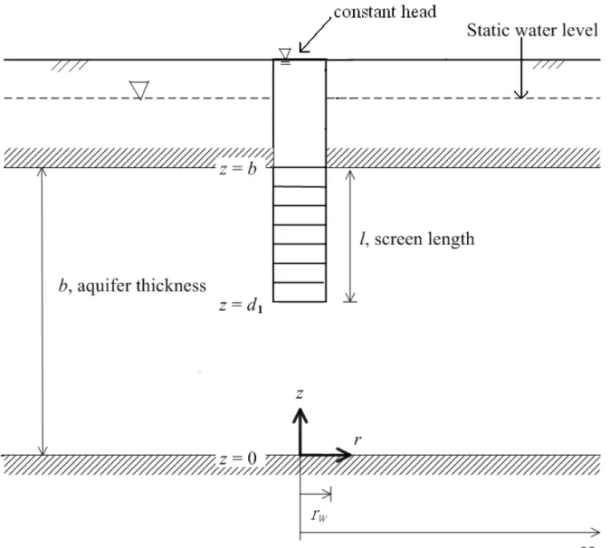
Figure 1. Schematic representation of a partially penetrating well with the screen extends

from the top of the aquifer in a confined aquifer………33

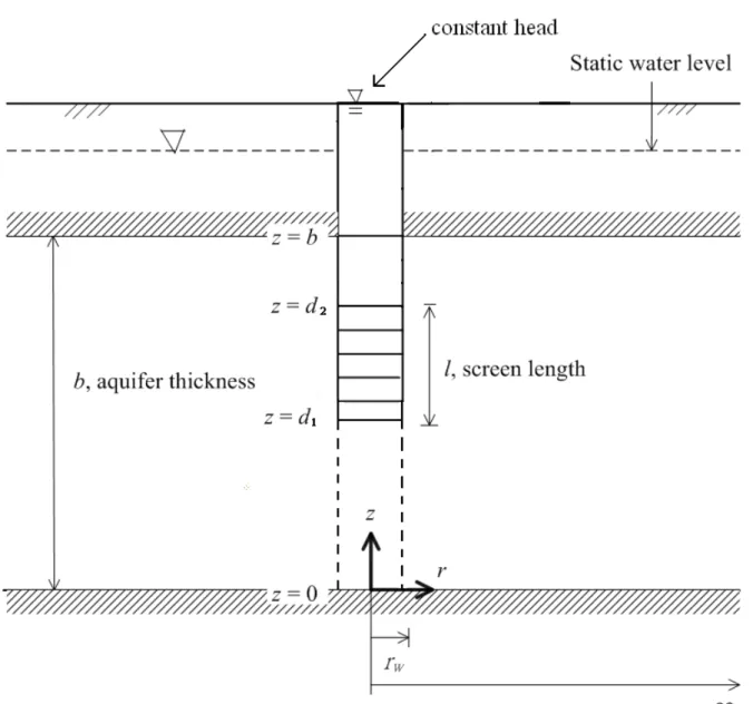
Figure 2. Schematic representation of a partially penetrating well with arbitrary location of

well screen in a confined aquifer………..34

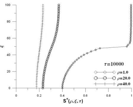
Figure 3. The drawdown distribution at dimensionless timeτ =1, 100, _{10 and} 4 _{τ =10}6 _for

various ρ………...35

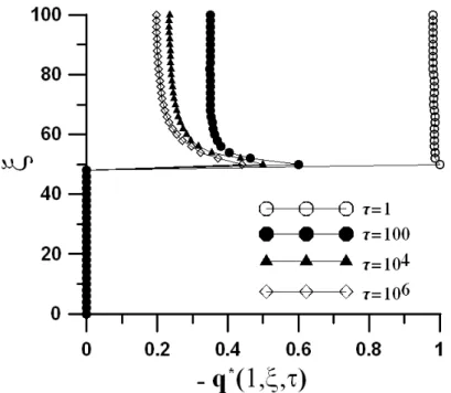
Figure 4. The distribution of flux along the well screen at different dimensionless time…….37

Figure 5. The spatial drawdown contours at dimensionless time τ =100, _{10 and} 3 4

10 =

τ ……… 38

Figure 6. The spatial drawdown contours at dimensionless time _{τ =10}5 _{for variousα}2_…39

Figure 7. The spatial drawdown contours at dimensionless time _{τ =10}6 _{for different screen}

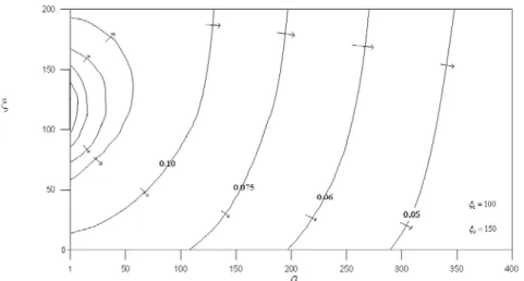
location with β =50. (ξ₁ =12.5 and ξ₂ =37.5; ξ₁ =25and ξ₂ =50 )….…40 Figure 8. The spatial drawdown contours as at dimensionless time _{τ =10}7 _{for 100}

1 =

ξ

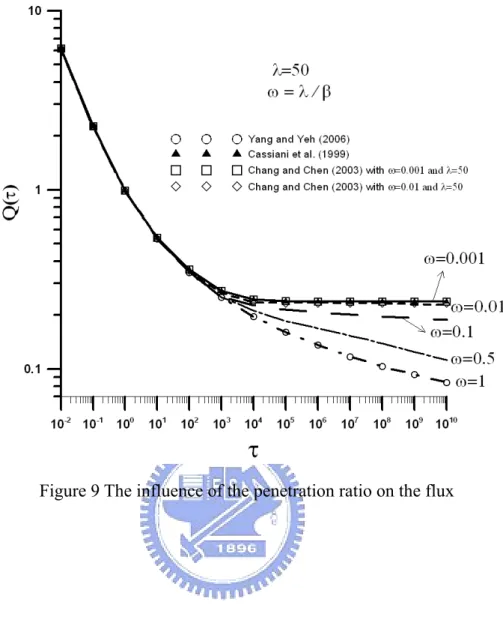
a n d ξ₂ =150… … … . . 4 1 Figure 9. The influence of the penetration ratio on the flux………..42

NOMENCLATURE

b : thickness of aquifer (L)

1

d : depth to bottom of the well screen (L)

2

d : depth to top of the well screen (L)

H(n,p) : )K1(λn)/K0(λn

r

K : radial hydraulic conductivity (LT-1)

z

K : vertical hydraulic conductivity (LT-1) )

(

0 ⋅

K : modified Bessel function of the second kind of zero order

) ( 1 ⋅

K : modified Bessel function of the second kind of first order

Kr : horizontal hydraulic conductivity of unconfined aquifer

Kz : vertical hydraulic conductivity of unconfined aquifer l : length of screen (L)

n : finite Fourier cosine transform parameter of ξ

p _{: Laplace transform parameter of} τ

) (cosu

P_{n : associated Legendre function}

) , , 1 ( * p

q ξ : dimensionless well bore flux in Laplace domain

) (

*

p

Q : dimensionless well discharge in Laplace domain r : radial distance (L)

w

r : well bore radius (L)

w

s : constant drawdown prescribed at the well (L) ) , , (r z t s : transient drawdown (L) ) , , ( * _{ρ ξ τ} s : dimensionless drawdown ) , , ( * _{ρ ξ τ}

s : dimensionless drawdown in Laplace domain

) , , ( ˆ* _{ρ ξ τ}

s

S : specific storage coefficient (L-1)

t _{: time (T)}

z : vertical distance (L)

2

α : K /_r K_z, anisotropy ratio

β : b /rw, dimensionless aquifer thickness

λ : l /r_w, dimensionless screen length n λ _{: (nπα/β)}2_{+ p} η _{: nπ/β} 1 μ : ξ₁π/β 2 μ : π(1−ξ₂/β)

ξ : z /rw, dimensionless vertical distance

1

ξ : d /1 rw

2

ξ : d /2 rw

ρ _: r /r_w, dimensionless radial distance

τ : _/ 2

w s rt S r

K , dimensionless time

ω _{: l /b, partial penetration ratio}

0

CHAPTER 1 INTRODUCTION

1.1 Background

Hydraulic parameters, e.g., hydraulic conductivity, specific storage and leakage factor,

are important for characterizing the aquifer and quantifying groundwater resources. Two

typical pumping tests (i.e. constant-head and constant-rate pumping tests) are widely

conducted by the hydrogeologists to determine the hydraulic parameters of the aquifer. In a

constant-rate test, the well is pumped for a significant length of time at a constant rate and at

least one observation is used to obtain the drawdown data. However, the pumped well may

be overdrawn if the aquifer has low permeability. Therefore, the constant-head test is

generally employed in this circumstance. During the test, the hydraulic head at the well is

kept constant throughout the test period and the transient flow rate across the wellbore is

measured at the same time. Rice [1998] mentioned that there are some merits in

constant-head tests. In recent years, owing to the numerous important issues in the

low-permeability aquifers, there has been an increasing interest in the study of constant-head

tests. Jones et al. [1992] and Jones [1993] discussed the practicality of constant-head tests

on wells completed in low-conductivity glacial till deposits. Mishra and Guyonnet [1992]

developed a method for analyzing observation-well response to constant-head test. For other

environmental applications, light nonaqueous phase liquids (LNAPL) are typically recovered

by wells held at constant drawdown [Murdoch and Franco, 1994]. The strategy for the

contaminated site is to hold a slight drawdown and remove LNAPL as it accumulates in the

well.

The wellbore storage plays an important role for estimating aquifer parameters in

constant-rate tests. However, the effect of wellbore storage can be neglected for

constant-head tests if the aquifer has low-conductivity and the radius of well is small.

Some aquifers are so thick that it is not justified to install a fully penetrating well. The

pumping test has to be performed in a partially penetrating well instead of fully penetrating

well. For example, the suggested length of screen is 6 m and the screen should be 1 m and 5

m below the water table at least for flood and dry seasons, respectively, for unconfined

aquifers in Taiwan. For confined aquifer, the location of the screen is adapted for the

purpose of the well. In addition, the partially penetrating well could be used in a pumping

test to evaluate the hydrologic parameter in heterogeneous aquifers. Therefore, the issues

involving partially penetrating well are studied in literatures [e.g., Cassiani and Kabala, 1998;

Cassiani et al., 1999; Yang and Yeh, 2005].

The drawdown data may be influenced by the well skin effect produced by well

description for such an aquifer system should treat the skin zone as a different formation zone

instead of using a skin factor. Thus, the aquifer system naturally becomes a two-zone

formation [see, e.g., Yang and Yeh, 2002; Yeh et al., 2003; Yang and Yeh, 2005; Yeh and Yang,

2006]. If the well skin effect is negligible in the model, the well loss can be ignored. The

fully penetrating well can be simulated as a Dirichlet (also called the first type) boundary

condition, and the relative models can be solved by the conventional integral transform

techniques [Hantush, 1964]. For partially penetrating well, the Dirichlet boundary condition

is suited to describe the drawdown along the well screen and the Neuman (second type)

boundary condition is specified along the casing. Thus, the boundary condition along the

well face in the partially penetrating well is a mixed type condition. The term “mixed-type”

boundary condition is used to distinguish this boundary condition from the “uniform”

Dirichlet and Neuman boundary condition or a combination of Dirichlet and Neuman

boundary conditions.

1.2 Objectives

The purpose of this study is to develop a new solution to a constant head test performed in a

partially penetrating well for arbitrary location of the well screen in an aquifer of finite

thickness in depth. The study is based on the following assumptions: (1) The aquifer is

the initial head is constant and uniform throughout the whole aquifer; (4) the well loss is not

considered in the system. Under these assumptions, this study will further compare the new

CHAPTER 2 LITERATURE REVIEW

Mixed boundary conditions are widely used to describe many boundary value problems

of mathematical physics. Such problems arise in potential theory and its numerous

applications to engineering, fracture mechanics, heat conduction, and many others. Only

limited analytical solutions to mixed boundary problems (MBPs) in the field of well

hydraulics have been found so far by special solution techniques including the dual

integral/series equation [Sneddon, 1966], Weiner-Hopf technique [Noble, 1958], and Green’s

function [Huang and Chang, 1984]. Most of the solutions to MBPs have been obtained

numerically or by approximate methods such as asymptotic analysis or perturbation

techniques. Yedder et al. [1994] studied the steady heat conduction in a square plate with

mixed boundary condition on a straight boundary using finite difference and control volume

methods. They overcame the difficulties encountered in singular cases and discussed the

convergence criteria used in the numerical treatment of these problems. Bassain et al. [1987]

indicated that under certain circumstances, the mixed condition gives rise to singular behavior

which cannot be adequately treated by numerical means alone. They discussed the

implications of the singular behavior due to the mixed boundary condition of the

adiabatic-isothermal type in the mathematical modeling heat transfer phenomena. Wilkinson

transient testing and obtained good results in a variety of well test problems of this type.

For the mathematical model under the mixed boundary condition in a confined aquifer of

semi-infinite thickness, Cassiani and Kabala [1998] used the dual integral equation method to

develop a Laplace domain solution that account for the effect of wellbore storage,

infinitesimal skin, aquifer anisotropy and infinite aquifer thickness under constant-rate tests.

Cassiani et al. [1999] further used the same method to develop the solutions in Laplace

domain suited for constant head pumping tests and double packer tests that treated as the

MBPs. Selim and Kirkham [1974] used the Gram-Schmidt orthonormalization method to

develop a steady state solution in a confined aquifer of finite horizontal extent. Similar

problems under the mixed boundary conditions also arise in the field of heat conduction.

Among others, Huang [1985] used the Weiner-Hopf technique to develop a solution in a

semi-infinite slab and Huang and Chang [1984] combined the Green’s function with

conformal mapping to develop the solution in an elliptic disk. The literatures listed above

are under the assumption that the domain which the mixed boundary condition occurs is

infinite. In reality, the thickness of aquifer is generally finite. Since the solutions in

Cassiani and Kabala [1998] and Cassiani et al. [1999] are based on the infinite aquifer

thickness assumption, they are only appropriate for the early time condition when the pressure

change caused by the constant-head pumping has not reached the bottom of the aquifer or for

Chang and Chen [2002] removed such constraints by assuming finite aquifer thickness and

treated the well skin effect as a skin factor. They also treated the boundary along the well

screen as a Cauchy (third type) boundary condition and replaced the mixed boundary by

homogeneous Neumann boundary. They considered the wellbore flux entering through the

well screen as unknown and discretized the screen length into M segments. Thus, the

discretization approach to deal with mixed boundary is numerical and their solution may be

inaccurate if an improper choice of M is made. In other words, only when M approaches

CHAPTER 3 METHODOLOGY

3.1 Partially penetrating: screen extends from the top of the aquifer

The water level is held as a constant at a preselected depth while precisely measuring

flow rate changes when conducting a constant-head test. Figure 1 shows a partially

penetrating well in a confined aquifer of finite extent with a thickness of b under a

constant-head test. The drawdown at the distance r from the well and the distance z from the

bottom of the aquifer at time t is denoted as s(r, z, t). The well screen extends form the top

of the aquifer (z = b) to z = d1 with a length of l. The hydraulic parameters of the aquifer are

horizontal hydraulic conductivity Kr, vertical hydraulic conductivity Kz, and specific storage

Ss. Since the flow velocities are so low and the pressure exerted by the atmosphere is more

or less constant at a site in groundwater situations the velocity energy and the pressure are not

taken into consideration in this study. Therefore, the governing equation for the drawdown

can be written as [Yang et al., 2006]

t s S z s K r s r r s Kr z s ∂ ∂ = ∂ ∂ + ∂ ∂ + ∂ ∂ 2 2 2 2 ) 1 ( (1)

Assuming that there is no flow toward to the bottom of the well, consequently a Dirichlet

boundary condition for a fixed drawdown specified along the well screen is:

w

w z t s

r

s( , , )= d₁≤z≤b (2a)

0 = ∂ ∂ =rw r r s 0≤z≤d₁ (2b)

Moreover, the initial condition and other boundary conditions are:

0 ) 0 , , (r z = s (3) 0 ) , , (∞ tz = s (4) and , 0 = ∂ ∂ z s z= ,0 z=b (5)

Equation (1) may be expressed in dimensionless terms as:

τ ξ α ρ ρ ρ ∂ ∂ = ∂ ∂ + ∂ ∂ + ∂ ∂ * 2 * 2 2 * 2 * 2 ₁ s s s s (6)

subject to the boundary and initial conditions written in dimensionless terms as

0 ) 0 , , ( * _{ρ ξ τ = =} s (7) 0 ) , , ( * _{ρ=∞ ξ τ =} s (8) 1 ) , , 1 ( * _{ρ= ξ τ =} s , ξ₁ ≤ξ ≤β (9a) 0 1 * = ∂ ∂ = ρ ρ s , 0≤ξ ≤ξ₁ (9b) , 0 * = ∂ ∂ ξ s ξ = ,0ξ =β (10) where s s/sw

* _{= is the dimensionless drawdown, (} 2₎

w s

r S r

tK

=

τ is the dimensionless time,

r

z K

K

=

2

α is the anisotropy ratio of the aquifer, β =b /rw is the dimensionless aquifer

thickness, ρ =r /rw and ξ =z /rw are dimensionless spatial coordinates, ξ1 =d /1 rw is the

mixed-type boundary value problem.

The detailed development for the solution of Eq. (6) with Eqs. (7) – (10) using dual

series equation and perturbation method is given in Appendix A. The solution for the

drawdown in Laplace domain can be written as:

) cos( ) , ( ) , 0 ( 2 1 ) , , ( 1 0 * _{ρ ξ ψ ψ ηξ} n n p n B p B p s

∑

∞ = + = (11) with η =(nπ)/β , ψ₀ =K₀( pρ)/K₀( p) and ψ_n =K₀(λ_nρ)/K₀(λ_n). The coefficients

in Eq. (11) can be calculated by the following equations

(

)

⎥ ⎦ ⎤ ⎢ ⎣ ⎡ _{Ω + − + Ω} ⋅ Ω + =

∑

∞ = − ) , ( 2 ) 1 ( 2 ) ( 4 ) ( 1 1 2 1 1 1 3 1 1 1 0 0 k C I k p p H p B k k k μ μ μ π μ (12) and π π μ μ μ π μ μ μ μ μ μ μ pn n dy dy y n df y n f p n f dy dy y n df y B H p dy dy y n df k y n f k B I k B k k k n ) sin( 2 ) , ( ) ( ) , ( ) ( 2 ) , ( ) ( ) , ( ) ( 2 1 ) , ( ) , ( ) , ( ) , ( 1 1 0 2 3 1 2 1 3 1 2 1 1 0 2 1 0 0 0 2 2 1 2 1 2 1 1 1 1 − ⎥ ⎦ ⎤ ⎢ ⎣ ⎡_{Ω ⋅ − Ω ⋅} + ⎥ ⎦ ⎤ ⎢ ⎣ ⎡ _{Ω ⋅ −Ω ⋅} + ⎥ ⎦ ⎤ ⎢ ⎣ ⎡_{Ω ⋅ − Ω ⋅} =

∫

∫

∫

∑

∞ = (13) with β π ξ μ₁ = ₁ / (14)

∫

= Ω x udu x u f x 0 1 1( ) ( , ) (15)

∫

= Ω x du ku x u f k x 0 1 2( , ) ( , )sin( ) (16)

∫

= Ω x du x u f x u f x 0 1 3 3( ) ( , ) ( , ) (17)

p n n ⎟⎟ + ⎠ ⎞ ⎜⎜ ⎝ ⎛ = 2 β πα λ (18) ) ( / ) ( ) , (n p Hn K₁ n K₀ n H = = λ λ (19) ) cos( ) 2 / cos( ) 2 / sin( 2 ) , ( 1 a x x a x f − = π (20)

[

(cos ) (cos )

]

) , ( ₁ 2 n a P a P a f = n + n− (21)

(

ln(1 cos( )) ln(1 cos( ))

)

4 1 ) , ( 3 x a a x a x f = − + − − − (22) ) , ( ) , (n p I n H n p I = n = −λn (23) and p n n ⎟⎟ + ⎠ ⎞ ⎜⎜ ⎝ ⎛ = 2 β πα λ (24) where K0 and K1 are the modified Bessel functions of the second kind with order zero and one,

respectively, and the Pn(cosa) is the associated Legendre function [Abramowitz and Stegun,

1970, p.335].

The flux entering the well screen and the total well discharge obtained using Eq. (11) are

respectively given as:

) cos( ) , ( ) , 0 ( 2 1 ) , , 1 ( ) , , 1 ( 1 0 * * _{λ ηξ} ρ ξ ξ n n n H p n B H p p B p s p q

∑

∞ = + = ∂ ∂ − = (25) and ) sin( ) , ( ) , 0 ( 2 1 / ) , , 1 ( ) ( ₁ 1 0 * 1 μ λ πλ β λ ξ ξ β ξ n H p n B n H p p B d p q p Q _{n n} n

∑

∫

= − ∞₌ = (26)

3.2 Partially penetrating: arbitrary location of the well screen

Figure 2 shows a schematic representation of a partially penetrating well in a confined

aquifer of finite extent with a finite thickness of b. The well screen which extends from

arbitrary location d1 to d₂ is of length l under a prescribed constant drawdown h_w. In other

words, the well screen can be set at any location along the well.

The boundary along the well screen is different from that in section 3.1, which can be written

as: w w z t s r s( , , )= d₁≤z≤d₂ (27) and 0 = ∂ ∂ =rw r r s 0≤z≤d₁, d₂ ≤z≤b (28)

The detail derivation for the solution with Eqs. (27) and (28) using Laplace transform,

finite Fourier cosine transform, and triple series equations method is given in Appendix B.

The solution for drawdown in an aquifer involving a partially penetrating well with arbitrary

location of well screen has the same expression as Eq. (11) and the coefficients B(0, p) and

B(n, p) are written as 0 0 ) , 0 ( ) , 0 ( ) , 0 ( D C p D p C p B + = + = (29) and n n D C p n D p n C p n B + = + = ( , ) ( , ) ) , ( (30)

(

)

⎥ ⎦ ⎤ ⎢ ⎣ ⎡ _{Ω + − + − Ω − Ω} ⋅ Ω + =

∑

∞ = − ) ( 2 ) , ( ) ( 2 ) 1 ( 2 ) ( 4 ) ( 1 1 1 0 0 1 2 1 1 1 3 1 1 1 0 0 μ μ μ μ π μ H p D k D C I k p p H p C k k k k (31) π π μ μ μ π μ μ μ μ λ μ μ μ pn n dy dy y n df y n f p n f dy dy y n df y D C H p dy dy y n df k y n f k D C I k C k k k k k n ) sin( 2 ) , ( ) ( ) , ( ) ( 2 ) , ( ) ( ) , ( ) ( ) ( 2 1 ) , ( ) , ( ) , ( ) , ( ) ( 1 1 0 2 3 1 2 1 3 1 2 1 1 0 2 1 0 0 0 0 2 2 1 2 1 2 1 1 1 1 − ⎥ ⎦ ⎤ ⎢ ⎣ ⎡_{Ω ⋅ − Ω ⋅} + ⎥ ⎦ ⎤ ⎢ ⎣ ⎡ _{Ω ⋅ −Ω ⋅} + + ⎥ ⎦ ⎤ ⎢ ⎣ ⎡_{Ω ⋅ − Ω ⋅} − =

∫

∫

∫

∑

∞ = (32)

(

)

_⎥⎦⎤ ⎢⎣ ⎡ _{Ω − − − Ω} Ω + =

∑

∞ = − ) , ( 2 ) ) 1 ( )( , ( 2 ) ( 1 _{2 2 0 0 1 2} 1 1 2 1 0 0 k I H D D pH k k H p D _k k _{k k k} k μ λ μ μ (33) and ⎥ ⎦ ⎤ ⎢ ⎣ ⎡ _{Ω ⋅ −Ω ⋅} − + ⎥ ⎦ ⎤ ⎢ ⎣ ⎡_{Ω ⋅ − Ω ⋅} ⋅ − − − =

∫

∫

∑

∞ = ) , ( ) ( ) , ( ) ( ) ( 2 1 ) , ( ) , ( ) , ( ) , ( ) ( 1 ) 1 ( ) 1 ( 2 2 2 1 0 2 1 0 0 0 0 2 2 2 2 2 2 1 2 2 μ μ μ μ λ μ μ n f dy dy y n df y C D H p dy dy y n df k y n f k C H D I k D _{k k k} k k k k n n (34) ) / 1 ( ₂ 2 π ξ β μ = − (35) The flux entering the well screen and the total well discharge are respectively given as:

) cos( 2 1 ) , , ( ) , , 1 ( 1 0 0 1 * * _{λ ηξ} ρ ξ ρ ξ ρ n n n n H B H p B p s p q

∑

∞ = = + = ∂ ∂ − = (36) and

[

sin( ) ( 1) sin( )

]

) ( 2 1 ) , , 1 ( 1 ) ( _{1 2} 1 1 0 0 * 2 1 μ μ λ λη ξ ξ λ ξ ξ n n H B H p B d p q p Q _{n n} n n n + − − = =

_∫

∑

∞ = − ₍₃₇₎

CHAPTER 4 RESULTS AND DISCUSSION

4.1 Simplified solution

When the well fully penetrates the entire thickness of the formation, i.e., ξ₁ is zero and

2

ξ equals β, the drawdown and the well discharge can be obtained using Eqs. (11) and (37), respectively, with coefficients in Eqs. (31) – (34) as

0 *_{(ρ,ξ, )} 1_ψ p p s = (38) and p H p Q( )= 0 (39)

Equations (38) and (39) are identical to the solutions of drawdown and flow rate in Laplace

domain given in Yang and Yeh [2006].

4.2 Numerical evaluations

Equation (11) contains single and double infinite series which consist of the summations

of multiplication of integrals, trigonometric functions, and the modified Bessel functions of

second kind. The integrals are in terms of trigonometric functions multiplying associated

Legendre functions. This solution involves numerous complicated mathematical functions.

Therefore, numerical approaches including the Gaussian quadrature [Gerald and Wheatley,

1989], Shanks’ transform and Stehfest method are proposed to evaluate the solution. The

integrals in Eq. (11). Since the oscillation and slow convergence of the multiplication terms,

the summations are difficult to evaluate accurately and efficiently. Therefore, the Shanks’

transform method [Shanks, 1955], a nonlinear iterative algorithm based on the sequence of

partial sums, is used to compute the summations in Eq. (11). This method has been

successfully devoted to efficiently computing the solutions arisen in the groundwater area [see,

e.g., Peng et al. 2002; Yeh et al. 2003]. In addition, the Stehfest algorithm [Stehfest, 1970]

with eight weighting factors is further employed to inverse the Laplace domain solution into

time domain solution. The proposed numerical approaches can accurately evaluate the

drawdown solution to the mixed-type boundary value problem for a flowing partially

penetrating well and the results are demonstrated in the following section.

4.3 Drawdown and well bore flux distribution

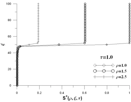
Figure 3 shows the dimensionless drawdown forβ =100, ξ₁=50, ξ₂ =100 and various ρ at τ =1, 100, _{10 and} 4 _{10 . As indicated in the figure, the dimensionless} 6

drawdown is constant along the well screen and decreases with increasing dimensionless

radial distance at τ =1 . In addition, the dimensionless drawdown increases with dimensionless time along the unscreened part of the well. Figure 4 shows the plots of the

flux along the well screen forβ =100, ξ₁ =50 and ξ₂ =100 at τ =1, 100, _{10 and} 4 _{10 .} 6

vertical flow is induced by the presence of well partial penetration and the maximum flux at

the screen edge occurs when the vertical flows enter the bottom of the well. The spatial

dimensionless drawdown contours at τ =100, _{10 and} 3 _{10 are plotted in Figure 5. The} 4

dimensionless drawdown increases with dimensionless time at a fixed radial distance and

flow is horizontal when the dimensionless radial distance is large than 80 and the

dimensionless time is _{10 . Figures 6(a) and 6(b) show the spatial dimensionless drawdown} 4

contours for various _α2 _{with 200} 1 =

ξ and ξ₂ =250 at _{τ =10}5 _{and demonstrates the}

influence of anisotropy on the dimensionless drawdown. The flow is almost horizontal at

lower part of the aquifer when the dimensionless radial distance is large than 400 for _α2₌₁

and the vertical flow appears at lower part of the aquifer for _α2_{=0.5. Figures 7(a) and 7(b)}

show the spatial dimensionless drawdown contours with same length of 50 but different

locations of well screen. In Figure 7(a), the screen is symmetric with ξ₁ =12.5 and

5 . 37 2 =

ξ and in Figure 7(b) the screen extends from the top of the aquifer with ξ₁ =25

and ξ₂ =50 at _{τ =10}5_{. Since the screen is symmetric about the middle line of the aquifer,}

the drawdown contours are symmetric as demonstrated in Figure 7(a). Figure 8 illustrates

the spatial dimensionless drawdown contours for ξ₁=100 and ξ₂ =150 at _{τ =10}7_{in an}

infinite aquifer. On the upper part of the aquifer, the direction of flow is downward when the

radial distance is far from the test well and it is upward when the radial distance is close to the

upward and then flows toward the bottom of the aquifer and the drawdown at the lower screen

ledge flows down toward the bottom of the aquifer.

4.4 Effect of penetration ratio

In order to explore the effect of partial penetration on the well discharge, Figure 9

illustrates the behavior of well discharge in response to four different penetration ratios

β λ

ω = / with λ =50. The well discharges responding to those four cases behave the same at the small time; however, it decreases with increasing penetration ratio at large time.

If the penetration ratio is smaller than 0.01, the well discharge of this study agrees with that of

constant head pumping test in Cassiani et al.[1999] in an aquifer of semi-infinite thickness.

In other words, if the aquifer thickness is greater than 100 times of the screen length, the

aquifer can be considered as a semi-infinite aquifer. As the penetration ratio is equal to 1,

the well discharge of this study is identical to that of Yang and Yeh [2006] for a fully

penetrating well. In addition, well discharges of this study agree with those of Chang and

Chen [2003] for ω =0.01 and ω =0.001 when λ =50. As indicated in Figure 9, there are no obvious differences in the well discharges in response to different penetration ratios

until _{τ =10}4_{. For the cases of ω =0.1 and ω =0.01, the flow caused by the partial}

penetration did not reach to the bottom of the aquifer before _{τ =10}4_{. The aquifer thickness}

01 . 0 =

ω is stabilized as τ increases to _{10 and the well discharge for} 6 _{ω =0.5 continues}

CHAPTER 5 CONCLUSIONS

This paper developed new semi-analytical solutions for the aquifer system in response

to the constant head test at a partially penetrating well in a confined aquifer of infinite radial

extent and finite vertical extent. The Laplace and finite cosine Fourier transforms is first

used to reduce the original partial differential equation with mixed-type boundary and initial

conditions for a partially penetrating well in an aquifer of finite thickness to the dual or triple

series equations.

The present solutions for a fully penetrating well in an aquifer of finite thickness are

identical to the solutions of the drawdown and well discharge given in Chen and Stone [1993].

It is found that the solution of Cassiani et al. [1999] for well response to a constant head

pumping test in a semi-infinite aquifer approximates the solution for the case where the

aquifer thickness of a finite aquifer is 100 times greater than the length of well screen. In

addition, the flux is non-uniformly distributed along the screen and with a local peak at the

edge, due to the vertical flow induced by well partial penetration.

The new semi-analytical solutions provide accurate description of the response of the

aquifer system to a constant head pumping test performed at a partially penetrating well in a

confined aquifer of infinite radial extent and finite vertical extent. Those solutions are

sensitivities of the input parameters in a mathematical model. In addition, the solution can

be used to calculate the flow rates during the constant-head test and plots specific drawdown

(drawdown divided by the flow rate) versus time to identify the hydraulic parameters if

coupling with an optimization approach in the analysis of aquifer data, and to verify a

APPENDIX A

The Laplace and finite cosine Fourier transforms are first used to solve the mixed-type

boundary value problem. The definition of Laplace transform is [Sneddon, 1972]：

[

]

_∫

∞ − = → = 0 * * *_{(ρ,ξ, ) (ρ,ξ,τ);τ (ρ,ξ,τ)} τ _τ d e s p s L p s p p (A1) where *( , , ) p

s ρ ξ is the dimensionless drawdown in Laplace domain. Taking the Laplace

transform of Eqs. (6) and (8) – (10) and using the initial condition in Eq. (7), the problem

reads: 0 1 * 2 * 2 2 * 2 * 2 = − ∂ ∂ + ∂ ∂ + ∂ ∂ s p s s s ξ α ρ ρ ρ (A2) 0 ) , , ( * _{=∞ =} p s ρ ξ _(A3) p p s*(ρ =1,ξ, )= 1 , ξ₁ ≤ξ ≤β (A4a) 0 1 * = ∂ ∂ = ρ ρ s , 0≤ξ ≤ξ₁ (A4b) , 0 * = ∂ ∂ ξ s _{ξ = ,ξ =β} 0 (A5)

In order to eliminate the ξ coordinate, the finite cosine Fourier transform is used as follows [Sneddon, 1972]:

[

→

]

=

_∫

= β ξ ηξ ξ ρ ξ ξ ρ ρ 0 * * *_{( , , ) ( , , ); ( , , )cos( )} ˆ _{n p F s p n s p d} s c (A6) where ˆ*( , , ) p n

s ρ is the dimensionless drawdown after finite cosine Fourier transform.

as 0 ˆ ˆ 1 ˆ * _{2 *} 2 * 2 = − ∂ ∂ + ∂ ∂ s s s n λ ρ ρ ρ (A7) with the boundary condition

0 ) , , ( ˆ* _{=∞ =} p n s ρ (A8)

where λn is defined in Eq. (24).

The general solution of Eq. (A7) with the boundary condition Eq. (A8) is [Carslaw and

Jaeger, 1959, p. 193] ) ( ) , ( ) , , ( ˆ 0 * _{ρ λ ρ} n K p n A p n s = _(A9)

where A(n,p) can be found from using the mixed-type boundary condition Eq. (A4). The

inverse of the finite cosine Fourier transform is [Sneddon, 1972, p.425]

) cos( ) , , ( ˆ 2 ) , 0 , ( ˆ 1 ) , , ( 1 * * *

∑

∞ = + = n p n s p s p s ρ ηξ β ρ β ξ ρ (A10) Thus, the solution in ξ domain obtained by inserting Eq. (A9) into Eq. (A10) is

) cos( ) ( ) , ( 2 ) ( ) , 0 ( 1 ) , , ( 1 0 0 *

∑

∞ = + = n n K p n A p K p A p s λ ρ ηξ β ρ β ξ ρ (A11)

with its derivative with respect toρ given by

) cos( ) ( ) , ( 2 ) ( ) , 0 ( 1 ) , , ( 1 1 1 *

∑

∞ = − − = ∂ ∂ n n nK p n A p K p p A p s _{λ λ ρ ηξ} β ρ β ξ ρ ρ (A12)

Substituting Eq. (A11) into Eq. (A4a) and Eq. (A12) into Eq. (A4b) results in a system of the

dual series equations (DSE)

p K p n A p K p A n n 1 ) cos( ) ( ) , ( 2 ) ( ) , 0 ( 1 1 0 0 +

∑

= ∞ = ηξ λ β β ,ξ1 ≤ξ ≤β (A13a) 0 ) cos( ) ( ) , ( 2 ) ( ) , 0 ( 1 1 1 1 +

∑

= ∞ = n n nK p n A p K p p A λ λ ηξ β β ,0≤ξ ≤ξ1 (A13b)

We define that β λ )/ ( ) , ( 2 ) , (n p A n p K₀ n B = (A14)

The DSE of (A13) can be arranged as [Sneddon, 1966, p.161]:

p nx p n B p B n 1 ) cos( ) , ( ) , 0 ( 2 1 1 = +

∑

∞ = , μ₁< x≤π (A15a)

∑

∑

∞ = ∞ = = + 1 1 ) cos( ) , ( ) , ( ) cos( ) , ( ) , 0 ( ) , 0 ( 2 1 k n kx p k B p k I nx p n nB p H p p B , 0≤ x≤μ₁ (A15b) with x=ξπ/β.

Our goal is to determine the coefficients B(0, p) and B(n, p) appearing in Eq. (A15). The

pair of dual series equations (DSE) can be solved by following the procedure given in Sneddon

[1966]. Assume that when 0≤ x≤μ₁

∫

∑

= ₋ + ∞ = 1 cos cos ) ( ) 2 cos( ) cos( 2 1 ₁ 1 0 μ x n n y x dy y h x nx B B (A16) where μ₁ =ξ₁π /β , )B₀ =B(0,p and Bn =B( pn, ).

The coefficient B0 and Bn in Eq. (A15) are respectively given by the equations [Sneddon, 1966,

p. 161, Eqs. (5.4.56) and (5.4.57)] ⎥⎦ ⎤ ⎢⎣ ⎡ =

∫

1 0 1 0 ( ) 2 2 π μ π h y dy B (A17) and

[

]

⎭ ⎬ ⎫ ⎩ ⎨ ⎧ ₊ =

∫

1 ₋ 0 1( ) (cos ) 1(cos ) 2 2 2 π μ π h y P y P y dy Bn n n (A18)

Integrating (A15b), one can obtain

∫

∫ ∑

∑

= ⎟ ⎠ ⎞ ⎜ ⎝ ⎛ = + ∞ = ∞ = x x n n n n n du u F du nu I B nx B x p H p B 0 0 1 1 0 ) ( ) cos( ) sin( ) , 0 ( 2 1 (A19)

Substituting Eqs. (A17) and (A18) into (A19), one can find that h1(y)satisfies the following

equation: [Sneddon, 1966, p. 161, Eq. (5.4.58)]

[

]

) sin( ) cos( 1 2 ) , 0 ( 2 1 ) ( sin ) (cos ) (cos 2 1 ) ( 1 1 1 0 0 1 1 0 1 nx du nu p x B p H p du u F nxdy y P y P y h n x n n n

∫

∑

∫

∑

∫

∞ = ∞ = − − − = + π μ μ π (A20)

The summation term on the left-hand side of Eq. (A20) can be expressed as [Sneddon, 1966, p.

59, Eq. (2.6.31)]

[

]

x y y x H x nx y P y P eav n n n cos cos ) ( ) 2 cos( sin ) (cos ) (cos 2 1 1 1 − − = +

∑

∞ = − (A21)

where )Heav( X is the Heaviside unit step function which is of different value for different

range of X such as ⎪⎩ ⎪ ⎨ ⎧ > = < = 0 1 0 2 / 1 0 0 ) ( X X X X Heav (A22)

Substituting (A21) into (A20), it yields

⎪⎭ ⎪ ⎬ ⎫ ⎪⎩ ⎪ ⎨ ⎧ − − = − −

∫

∑

∫

∫

∞ = ) sin( ) cos( 1 2 ) , 0 ( 2 1 ) ( 2 sec cos cos ) ( ) ( 1 1 1 0 0 0 1 _{nu du nx} p x B p H p du u F x dy x y y x H y h n x π μ μ π (A23)

Using the property of Heaviside unit step function in Eq. (A22), an equivalent integral

equation of (A23) can be obtained

⎪⎭ ⎪ ⎬ ⎫ ⎪⎩ ⎪ ⎨ ⎧ − − = −

∫

∑

∫

∫

∞ = ) sin( ) cos( 1 2 ) , 0 ( 2 1 ) ( 2 sec cos cos ) ( 1 1 0 0 0 1 _{nu du nx} p x B p H p du u F x dy x y y h n x x π μ π 1 0≤ x<μ 　 　 　 (A24) ) (

∫

∫

∑

∫

_⎪⎭⎪⎬⎫ ⎪⎩ ⎪ ⎨ ⎧ − − − = ∞ = y n x dx nx du nu p x B p H p du u F y x x dy d y h 0 1 0 0 1 cos( ) sin( ) 1 2 ) , 0 ( 2 1 ) ( cos cos ) 2 / sin( 2 ) ( 1 π μ π π (A25)

By integrating Eq. (A25) and substituting it into Eqs. (A17) and (A18), the coefficients B0

and Bn can be expressed as Eqs. (12) and (13), respectively.

For computational convenience, the coefficients can be written in the matrix form as

⎥ ⎥ ⎥ ⎥ ⎥ ⎥ ⎦ ⎤ ⎢ ⎢ ⎢ ⎢ ⎢ ⎢ ⎣ ⎡ + ⎥ ⎥ ⎥ ⎥ ⎥ ⎥ ⎦ ⎤ ⎢ ⎢ ⎢ ⎢ ⎢ ⎢ ⎣ ⎡ ⎥ ⎥ ⎥ ⎥ ⎥ ⎥ ⎦ ⎤ ⎢ ⎢ ⎢ ⎢ ⎢ ⎢ ⎣ ⎡ = ⎥ ⎥ ⎥ ⎥ ⎥ ⎥ ⎦ ⎤ ⎢ ⎢ ⎢ ⎢ ⎢ ⎢ ⎣ ⎡ + + + + + + + + 1 3 2 1 2 1 0 1 , 1 3 , 1 2 , 1 1 , 3 33 32 1 , 2 23 22 1 , 1 13 12 2 1 0 0 0 0 0 n n n n n n n n n n Z Z Z Z B B B B X X X X X X X X X X X X B B B B # # " # % # # # " " " # (A26) with ⎥ ⎦ ⎤ ⎢ ⎣ ⎡ _{Ω ⋅} − _{−Ω ⋅ −} =

∫

( ) ( 1, ) ( ) ( 1, ) 2 1 1 2 1 1 0 2 1 0 1 1 μ μ μ i f dy dy y i df y H p X_i (A27) ⎥ ⎦ ⎤ ⎢ ⎣ ⎡ _{Ω ⋅} − _{−Ω ⋅ −} + ⎥ ⎦ ⎤ ⎢ ⎣ ⎡_{Ω − ⋅ − − Ω − ⋅} − − =

∫

∫

− ) , 1 ( ) ( ) , 1 ( ) ( 2 1 ) , 1 ( ) 1 , ( ) , 1 ( ) 1 , ( ) 1 ( 1 1 2 1 1 0 2 1 0 0 2 2 1 2 1 2 1 1 1 μ μ μ μ μ μ i f dy dy y i df y H p dy dy y i df i y i f i I j X_{ij j} (A28) ) ( 1 ) 1 ( 2 ) ( 4 1 1 0 1 1 3 1 _μ μ μ π Ω + − + Ω = H p p p Z (A29) p i i dy dy y i df y i f p Z_i π μ μ μ π μ ) 1 ( ) ) 1 sin(( 2 ) , 1 ( ) ( ) , 1 ( ) ( 2 1 0 2 3 1 2 1 3 1 − − − ⎥ ⎦ ⎤ ⎢ ⎣ ⎡_{Ω ⋅ − − Ω ⋅} − =

∫

(A30)

APPENDIX B

Similar to the procedure in Appendix A, the problem with the boundary in Eqs. (27) and

(28) results in a set of triple series equations as

p nx p n B p B n 1 ) cos( ) , ( ) , 0 ( 2 1 1 = +

∑

∞ = , μ₁< x≤π −μ₂ (B1a) 0 ) cos( ) , ( ) , 0 ( ) , 0 ( 2 1 1 = +

∑

∞ = n n nH nx p n B p H p p B λ , 0≤ x≤μ₁, π −μ₂ ≤x≤π (B1b)

We split Eq. (B1) into the following equations

0 ) cos( ) ( ) , 0 ( ) ( 2 1 1 0 0+ +

∑

+ = ∞ = n n n n n D H nx C p H p D C λ , 0≤ x≤μ₁ (B2a) p nx C C n n 1 ) cos( 2 1 1 0+

∑

= ∞ = , μ₁< x≤π (B2b) 0 ) cos( 2 1 1 0+

∑

= ∞ = n n nx D D , 0< x≤π −μ₂ (B3a) 0 ) cos( ) ( ) , 0 ( ) ( 2 1 1 0 0+ +

∑

+ = ∞ = n n n n n D H nx C p H p D C λ , π −μ₂ ≤x≤π (B3b)

Equations (B2) and (B3) can be regarded as dual series relations by means of which the

coefficients C0, D0, Cn and Dn can be determined.

The pair of dual series equations (DSE), i.e., Eq. (B2), can be solved by the procedure

⎥ ⎥ ⎥ ⎥ ⎥ ⎥ ⎦ ⎤ ⎢ ⎢ ⎢ ⎢ ⎢ ⎢ ⎣ ⎡ + ⎥ ⎥ ⎥ ⎥ ⎥ ⎥ ⎦ ⎤ ⎢ ⎢ ⎢ ⎢ ⎢ ⎢ ⎣ ⎡ ⎥ ⎥ ⎥ ⎥ ⎥ ⎥ ⎦ ⎤ ⎢ ⎢ ⎢ ⎢ ⎢ ⎢ ⎣ ⎡ + ⎥ ⎥ ⎥ ⎥ ⎥ ⎥ ⎦ ⎤ ⎢ ⎢ ⎢ ⎢ ⎢ ⎢ ⎣ ⎡ ⎥ ⎥ ⎥ ⎥ ⎥ ⎥ ⎦ ⎤ ⎢ ⎢ ⎢ ⎢ ⎢ ⎢ ⎣ ⎡ = ⎥ ⎥ ⎥ ⎥ ⎥ ⎥ ⎦ ⎤ ⎢ ⎢ ⎢ ⎢ ⎢ ⎢ ⎣ ⎡ + + + + + + + + + + + + + + + + 1 3 2 1 2 1 0 1 , 1 3 , 1 2 , 1 1 , 1 1 , 3 33 32 31 1 , 2 23 22 21 1 , 1 13 12 11 2 1 0 1 , 1 3 , 1 2 , 1 1 , 3 33 32 1 , 2 23 22 1 , 1 13 12 2 1 0 0 0 0 0 n n n n n n n n n n n n n n n n n n n Z Z Z Z D D D D Y Y Y Y Y Y Y Y Y Y Y Y Y Y Y Y C C C C X X X X X X X X X X X X C C C C # # " # % # # # " " " # " # % # # # " " " # (B4) with ⎥ ⎦ ⎤ ⎢ ⎣ ⎡ _{Ω ⋅} − _{−Ω ⋅ −} =

∫

( ) ( 1, ) ( ) ( 1, ) 2 1 1 2 1 1 0 2 1 0 1 1 μ μ μ i f dy dy y i df y H p X_i (B5) ⎥ ⎦ ⎤ ⎢ ⎣ ⎡ _{Ω ⋅} − _{−Ω ⋅ −} + ⎥ ⎦ ⎤ ⎢ ⎣ ⎡_{Ω − ⋅ − − Ω − ⋅} − − =

∫

∫

− ) , 1 ( ) ( ) , 1 ( ) ( 2 1 ) , 1 ( ) 1 , ( ) , 1 ( ) 1 , ( ) 1 ( 1 1 2 1 1 0 2 1 0 0 2 2 1 2 1 2 1 1 1 μ μ μ μ μ μ i f dy dy y i df y H p dy dy y i df i y i f i I j X_{ij j} (B6) ) ( 1 ) ( 1 1 0 1 1 0 11 _μ μ Ω + Ω − = H p H p Y (B7) ) ( 1 ) 1 , ( ) 1 ( 2 1 1 0 1 2 1 1 1 _μ μ λ Ω + − Ω − − = − − H p j H j Y j j j (B8) ⎥ ⎦ ⎤ ⎢ ⎣ ⎡ _{Ω ⋅} − _{−Ω ⋅ −} =

∫

( ) ( 1, ) ( ) ( 1, ) 2 1 1 2 1 1 0 2 1 0 1 1 μ μ μ i f dy dy y i df y H p Y_i (B9) ⎥ ⎦ ⎤ ⎢ ⎣ ⎡ _{Ω − ⋅} − _{−Ω − ⋅ −} − = − −

∫

( , 1) ( 1, ) ) , 1 ( ) 1 , ( ) 1 ( 1 1 2 1 2 0 2 2 1 1 1 μ μ λ μ dy j f i dy y i df j y H j Y_{ij j j} (B10) ) ( 1 ) 1 ( 2 ) ( 4 1 1 0 1 1 3 1 _μ μ μ π Ω + − + Ω = H p p p Z (B11)

p i i dy dy y i df y i f p Z_i π μ μ μ π μ ) 1 ( ) ) 1 sin(( 2 ) , 1 ( ) ( ) , 1 ( ) ( 2 1 0 2 3 1 2 1 3 1 − − − ⎥ ⎦ ⎤ ⎢ ⎣ ⎡_{Ω ⋅ − − Ω ⋅} − =

∫

(B12)

where i and j goes from 1 to n.

Similarly, Eq. (B3) can be solved by setting x'=π −x and D_n'=(−1)nD_n. Equation

(B3) is rewritten as 0 )' cos( ' ' 2 1 1 0 +

∑

= ∞ = n n nx D D , μ₂ < 'x ≤π (B13a) 0 ) ' cos( ) ) 1 ( ' ( ) ' ( 2 1 1 0 0 0 + +

∑

+ − = ∞ = n n n n n n C H nx D H p C D λ , 0≤ x'≤μ₂ (B13b)

and the coefficients D and ₀ D are n

⎥ ⎥ ⎥ ⎥ ⎥ ⎥ ⎦ ⎤ ⎢ ⎢ ⎢ ⎢ ⎢ ⎢ ⎣ ⎡ ⎥ ⎥ ⎥ ⎥ ⎥ ⎥ ⎦ ⎤ ⎢ ⎢ ⎢ ⎢ ⎢ ⎢ ⎣ ⎡ + ⎥ ⎥ ⎥ ⎥ ⎥ ⎥ ⎦ ⎤ ⎢ ⎢ ⎢ ⎢ ⎢ ⎢ ⎣ ⎡ ⎥ ⎥ ⎥ ⎥ ⎥ ⎥ ⎦ ⎤ ⎢ ⎢ ⎢ ⎢ ⎢ ⎢ ⎣ ⎡ = ⎥ ⎥ ⎥ ⎥ ⎥ ⎥ ⎦ ⎤ ⎢ ⎢ ⎢ ⎢ ⎢ ⎢ ⎣ ⎡ + + + + + + + + + + + + + + + n n n n n n n n n n n n n n n n n n C C C C YY YY YY YY YY YY YY YY YY YY YY YY YY YY YY YY D D D D XX XX XX XX XX XX XX XX XX XX XX XX D D D D # " # % # # # " " " # " # % # # # " " " # 2 1 0 1 , 1 3 , 1 2 , 1 1 , 1 1 , 3 33 32 31 1 , 2 23 22 21 1 , 1 13 12 11 2 1 0 1 , 1 3 , 1 2 , 1 1 , 3 33 32 1 , 2 23 22 1 , 1 13 12 2 1 0 0 0 0 0 (B14)

with the elements

) ( 1 ) 1 , ( ) 1 ( ) 1 ( 2 2 1 0 2 2 1 1 1 _μ μ Ω + − Ω − − = − − H p j I j XX j j j (B15) ⎥ ⎦ ⎤ ⎢ ⎣ ⎡_{Ω − ⋅ − − Ω − ⋅} − − − − = − − ₋

_∫

dy dy y i df j y i f j I j XX _j j i ij 2 0 2 2 2 2 2 2 1 1 1 _{( 1, )} ) 1 , ( ) , 1 ( ) 1 , ( ) 1 ( ) 1 ( ) 1 ( 2 μ μ μ π (B16) ) ( 1 ) ( 2 1 0 2 1 0 11 _μ μ Ω + Ω − = H p H p YY (B17) ) ( 1 ) 1 , ( ) 1 ( 2 2 1 0 2 2 1 1 1 _μ μ λ Ω + − Ω − − = − − H p j H j YY j j j (B18)

⎥ ⎦ ⎤ ⎢ ⎣ ⎡ _{Ω ⋅} − _{−Ω ⋅ −} − = −

∫

( ) ( 1, ) ( ) ( 1, ) 2 ) 1 ( 2 2 2 1 0 2 1 0 1 1 2 μ μ μ i f dy dy y i df y H p YY i i (B19) ⎥ ⎦ ⎤ ⎢ ⎣ ⎡ _{Ω − ⋅} − _{−Ω − ⋅ −} − − − = − −

∫

− − ) , 1 ( ) 1 , ( ) , 1 ( ) 1 , ( ) 1 ( ) 1 ( ) 1 ( 2 2 2 2 0 2 2 1 1 1 1 2 μ μ λ μ dy j f i dy y i df j y H j YY _{j j} i j ij (B20)

REFERENCES

Abramowitz, M., and I. A. Stegun (1970), Handbook of Mathematical Functions, Dover Publications, New York.

Bassani, J. L., M.W. Nansteel, and M. November (1987), Adiabatic-isothermal mixed boundary conditions in heat transfer, J Heat Mass Transfer., 30, 903-909.

Boridy, E., 1990. A perturbation approach to mixed boundary-value spherical problems, J.

Appl. Phys., 67, 6682-6666.

Carslaw, H. S., and J. C. Jaeger (1959), Conduction of heat in solids, 2nd Ed., Clarendon, Oxford.

Cassiani, G., and Z. J. Kabala (1998), Hydraulics of a partially penetrating well: solution to a mixed-type boundary value problem via dual integral equations, J. Hydrol., 211, 100-111.

Cassiani, G., Z. J. Kabala, and M.A. Medina Jr (1999), Flowing partially penetrating well: solution to a mixed-type boundary value problem, Adv. Water Resour, 23, 59-68.

Chang, C. C., and C.S. Chen (2002), An integral transform approach for a mixed boundary problem involving a flowing partially penetrating well with infinitesimal well skin,

Water Resour. Res., 38(6), 1071.

Chang, C. C., and C.S. Chen (2003), A flowing partially penetrating well in a finite-thickness aquifer: a mixed-type initial boundary value problem, J. Hydrol., 271, 101-118.

Chang, Y. C. and H. D. Yeh (2009) New solutions to the constant-head test performed at a partially penetrating well, J. Hydrol., doi:10.1016/j.jhydrol.2009.02.016

Gerald, C. F. and P. O. Wheatley (1989), Applied numerical analysis, 4th ed., Addison-Wesley, California.

Hantush, M. S. (1964), Hydraulics of wells. Advances in Hydroscience, 1, edited by V.T. Chow, Academic, San Diego, Calif., 309-343.

Hung, S. C. and Y. P. Chang (1984), Anisotropic heat conduction with mixed boundary conditions, J. Heat Transfer, 106, 646-648.

Hung, S. C. (1985), Unsteady-state heat conduction in semi-infinite regions with mixed-type boundary conditions, J. Heat Transfer, 107, 489-491.

Jones, L., T. Lemar, and C.T. Tsai (1992), Results of two pumping tests in Wisconsin age weathered till in Iowa, Ground Water, 30(4), 529-538.

Jones, L., T. (1993), A comparison of pumping and slug tests for estimating the hydraulic conductivity of unweathered Wisconsin age till in Iowa, Ground Water, 31(6), 896-904.

Mishra, S. and D. Guyonnet (1992), Analysis of observation-well response during constant-head testing, Ground Water, 32(6), 949-957.

Murdoch, L.D., and J. Franco (1992), The analysis of constant drawdown wells using instantaneous source functions, Water Resour. Res, 30(1), 117-127.

Noble, B. (1958), Methods based on the Wiener-Hopf techniques, Pergamon Press, New York.

Peng, H. Y., H. D. Yeh, and S. Y. Yang (2002), Improved numerical evaluation for the radial groundwater flow equation, Adv. Water Resour., 25(6), 663-675.

Rice, J.B (1998) Constant drawdown aquifer tests: an alternative to traditional constant rate tests, Ground Water Monit. R., 18(2), 76-78.

Shanks D. (1955), Non-linear transformations of divergent and slowly convergent sequence, J.

Math. Phys., 34, 1-42.

Slim, M. S., and D. Kirkham (1974), Screen theory for wells and soil drainpipes, Water

Resour. Res., 10(5), 1019-1030.

Sneddon, I.N. (1966), Mixed boundary value problems in potential theory, North-Holland, Amsterdam.

Sneddon, I.N. (1972), The use of integral transforms, McGraw-Hill, New York, 540pp.

Wilkinson, D., and P. S. Hammond (1990), A perturbation method for mixed boundary-value problems in pressure transient testing, Trans Porous Media, 5(6), 609-636.

Yang, S. Y., and H. D.Yeh (2002), Solution for flow rates across the wellbore in a two-zone confined aquifer, J. Hydraul. Eng. ASCE, 128(2), 175-183.

Yang, S. Y., and H. D. Yeh (2005). Laplace-domain solutions for radial two-zone flow equations under the conditions of constant-head and partially penetrating well, J.

Hydraul. Eng. ASCE, 131(3), 209-216.

Yang, S.Y., and H. D. Yeh (2006), A novel analytical solution for constant-head test in a patchy aquifer, Int. J. Numer. Anal. Methods Geomech, 30(12), 1213-1230, doi:10.1002/nag.523.

Yedder, R. B., and E. Bilgen (1994), On adiabatic-isothermal mixed boundary conditions in heat transfer, Warme Stoffubertragung, 29, 457-460.

Yeh, H. D., S. Y. Yang, and H. Y. Peng (2003), A new closed-form solution for a radial two-layer drawdown equation for groundwater under constant-flux pumping in a finite-radius well, Adv. Water Res., 26(7), 747-757.

Yeh, H. D., and S. Y. Yang (2006), A novel analytical solution for a slug test conducted in a well with a finite-thickness skin, Adv. Water Resour., 29(10), 1479-1489, doi:10.1016/j.advwatres.2005.11.002.

Figure 1 Schematic representation of a partially penetrating well with the screen extends from the top of the aquifer in a confined aquifer

Figure 2 Schematic representation of a partially penetrating well with arbitrary location of well screen in a confined aquifer

Figure 3a The drawdown distribution at dimensionless time for various ρ

Figure 3c The drawdown distribution at dimensionless timeτ =_{10 for various} 4 _ρ

Figure 5(a) The spatial drawdown contours at dimensionless time τ =100

Figure 5(b) The spatial drawdown contours at dimensionless time τ =₁₀ 3

Figure 6(a) The spatial drawdown contours at dimensionless time _{τ =10}5 _{for α}2 _=1.0

Figure 7(a) The spatial drawdown contours at dimensionless time _{τ =10}6 _{for 12.5} 1 = ξ and 5 . 37 2 = ξ with β =50

Figure 7(b) The spatial drawdown contours at dimensionless time _{τ =10}6 _{for 25} 1 =

ξ and

50 2 =

Figure 8 The spatial drawdown contours as at dimensionless time _{τ =10}7 _{for 100} 1 = ξ and 150 2 = ξ

VITA (個人簡歷)

姓 名 張雅琪 性 別 女 生 日 民國69 年 03 月 14 日 1998-2002 學士，交通大學土木工程學系 2002-2003 交通大學環境工程研究所碩士班 2003-2009 交通大學環境工程研究所博士班 學經歷

2007-2008 Visiting Scholar, Environmental Science and Engineering, University of North Carolina, USA

行動電話 0988314404

通訊電話 03-5712121#55527

通訊地址 300 新竹市交通大學環境工程研究所

PUBLICATION LIST

(A) Journal Papers

1. Yeh, H. D., and Y. C. Chang, 2006, New Analytical Solutions for Groundwater Flow in Wedge-shaped Aquifers with Various Topographic Boundary Conditions, Vol. 29, No. 3, 471-480, Advances in Water Resources. (SCI )

2. Y. C. Chang and H. D. Yeh, 2007, Optimum Allocation for Soil Contamination

Investigations in Hsinchu, Taiwan by Double Sampling, Soil Science Society of America

Journal, 71(5), 1585-1592, doi: 10.1061/sssaj1006.0130. (SCI)

3. Y. C. Chang, H. D. Yeh and Y. C. Hung, 2008, Determination of the parameter pattern and values for a one-dimensional multi-zone unconfined aquifer, Hydrogeology Journal, 16, 205-214. doi :10.1007/s10040-007-0228-3 (SCI)

4. Y. C. Chang and H. D. Yeh, 2007, Analytical solution for groundwater flow in an anisotropic sloping aquifer with arbitrarily located multiwells, Journal of Hydrology, 347, 143-152, 10.1016/j.jhdrol.2007.09.012. (SCI)

5. H. D. Yeh, Y. C. Chang and V. A. Zlotnik, 2008, Stream Depletion in Wedge-Shaped Aquifers, Journal of Hydrology, 349, 501-511. (SCI)

6. H. D. Yeh, S. B. Wen, Y. C. Chang and C. S. Lu, 2008, A new approximate solution for chlorine decay in pipes, Water Research, 42, 2787-2795. (SCI)

7. Chang, Y. C., H. D. Yeh, 2009, New solutions to the constant-head test performed at a partially penetrating well. Journal of Hydrology, doi:10.1016/j.jhydrol.2009.02.016 (SCI; IF:2.161)

8. Chang, Y. C., H. D. Yeh, 2009, Solutions for mixed boundary value problem in a constant-head test aquifer. Water Resources Research (In review)

9. Chang, Y. C., H. D. Yeh, K. F. Liang and M. C. T. Kuo, 2009, Scale dependency of fractional flow dimension in a fractured formation, Journal of Hydrology (In

10. Chang, Y. C., H. D. Yeh, Solutions for radial two-zone flow in unconfined aquifer under constant-head test. (In preparation)

11. Chang, Y. C., H. D. Yeh, G. Y. Chen, The flow rate across the wellbore in a two-zone unconfined aquifer. (In preparation)

(B) Conference papers 1. 張雅琪、葉弘德，92 年 4 月，離群值的檢定―以新竹市土壤污染數據為對象，第四 屆環境管理研討會, 嘉義，台灣，論文集光碟版 2002. 2. 張雅琪、葉弘德，92 年 11 月，使用雙重採樣法決定最佳採樣樣本數─以新竹市土壤 污染數據為對象，環工學會第十五屆年會及第一屆土壤與地下水技術研討會，國立中 興大學，台中，論文摘要集頁，論文集光碟版。 3 張雅琪、葉弘德，楔形含水層在定水頭邊界條件下之解析解，第 14 屆水利工程研討會, 新竹，台灣， 2004. 4. 張雅琪、葉弘德，93 年 10 月，水平多層自由含水層之地下水流研析，九十三年度農 業工程研討會，中國農業工程學會，桃園，論文摘要集 245 頁，論文集光碟版 1523-1529 頁。

5. Yeh, H. D., Y. C. Chang, and Y. C. Huang, 2005, Identifying horizontal multi-zone unconfined aquifer parameters using simulated annealing, AOGS 2nd annual meeting, Singapore, 58-HS-A0504. 6. 張雅琪、葉弘德，94 年月，應用多變量統計分析近海工業區之地下水污染，第九屆 土壤與地下水污染整治研討會，台北，論文集203～214 頁。 7. 張雅琪、葉弘德，94 年 9 月，楔形含水層在不同邊界條件下之地下水流研析，九十 四年電子計算機於土木水利工程應用研討會，中國土木水利工程學會，國立成功大 學，台南，論文集(III)491-496 頁。 8. 張雅琪、葉弘德，94 年 11 月，應用多變量統計分析地下水污染源:以台灣南部某污 染場址為案例，九十四年度農業工程研討會，中國農業工程學會，桃園，論文摘要集 111 頁，論文集光碟版。