1
國 立 交 通 大 學
管理科學系碩士班
碩士論文
台灣證券市場權益風險溢酬之估測
_比較 GARCH-M、移動視窗和 MIDAS 模型
Estimation of Equity Risk Premiums in Taiwan Security
Market: Comparison in Using GARCH-M, Rolling
Window and MIDAS Model
研 究 生:楊喜媛
指導教授:洪志洋 博士
王耀德 博士
2
台灣證券市場權益風險溢酬之估測
_比較 GARCH-M、移動視窗和 MIDAS 模型
Estimation of Equity Risk Premiums in Taiwan Security Market:
Comparison in Using GARCH-M, Rolling Window and MIDAS Model
研 究 生:楊喜媛 指導教授:洪志洋 博士 王耀德 博士 Student:Sii-Yuan Yang Advisor:Chih-Young Hung Yau-De Wang 國 立 交 通 大 學 管 理 科 學 系 碩 士 班 碩 士 論 文
A Thesis Submitted to Institute of Management Science
College of Management
National Chiao Tung University
in Partial Fulfillment of the Requirements
for the Degree of
Master in Business Administration
June 2012
Hsinchu, Taiwan, Republic of China
i
台灣證券市場權益風險溢酬之估測
_比較 GARCH-M,移動視窗和 MIDAS 模型
學生:楊喜媛 指導教授:洪志洋 王耀德 國立交通大學管理科學系碩士班中文摘要
本篇論文使用 Ghysel (2005)所提出混合數據抽樣模型(Mixed Data Sampling), 探討台灣證券交易市場的權益風險溢酬,在引入市場報酬的條件期望值和條件變 異數下,以跨期資本資產定價模型為基礎來進行估計與預測。樣本期間自 2006 年 1 月至 2010 年 12 月,以股票報酬之條件變異數作為風險替代變數,預測對象 是以月頻率為單位,觀察資料則為日/週頻率,針對不同的權重函數和波動因子, 進行和 GARCH-in-mean 模型與移動視窗模型之比較。 實證結果發現:(1) 此樣本期間之風險和權益風險溢酬有負向關係存在。(2) MIDAS 模型在時間序列資料的迴歸估計能力較顯著,其次是移動視窗法,且樣 本外資料的預測誤差偏小,表示預測能力良好。(3) 根據不同的波動因子和抽樣 頻率,以日頻率報酬資料的平方多項式有著較顯著估計結果。有別於傳統研究方 法,混合數據抽樣模型最大特點為採用不同頻率資料,配適出最佳迴歸模型,以 此估計證券市場的條件變異和風險報酬。 關鍵字:權益風險溢酬、混合數據抽樣模型,跨期資本資產定價模型,自我 相關條件異質變異模型、風險報酬抵換
ii
Estimation of Equity Risk Premiums in Taiwan Security Market:
Comparison in Using GARCH-M, Rolling Window and MIDAS
Model
Student:Sii-Yuan Yang Advisor:Chih-Young Hung
Yau-De Wang
Institute of Management Science
National Chiao Tung University
Abstract
This paper investigates risk premiums of Taiwan Stock Exchange Capitalization
Weighted Stock Index (TAIEX) by using Ghysel’s mixed data sampling (MIDAS)
model which is a new regression regarding volatility estimation. We study the
intertemporal relation between conditional mean and conditional variance of the
aggregate stock market return. Compared with various approaches such as
GARCH-in-mean, rolling window and MIDAS models, we find that: (i) We support
for a negative relation between risk and equity risk premium in TSEC weighted index
during the period 2006 - 2010. (ii) MIDAS is more convincing in predicting
regression for sampled time-series data. (iii) Empirical results show out-sample
forecasting ability of MIDAS model also performs well. Specifically, it has smaller
forecasting error. (iv) Under MIDAS model of different volatility predictors and
different sampling frequencies, a squared premium polynomial with daily frequency
data has better estimation.
Keywords:Equity Risk Premium, GARCH-M, ICAPM, MIDAS, Risk-Return
iii
致謝
終於要畢業了! 研究所這兩年光景或許不長,但絕對是我人生中截至目前最重要的決定之一。 首先要感謝最愛我的父母親,在我決定辭掉銀行的工作,準備考試進修的時候, 全力地支持我,儘管那段決定過程中仍有一點小波折,但對於你們的無悔付出和 鼓勵,女兒真的是點滴在心頭。還有我親愛的弟弟,感謝你的一語驚醒夢中人, 讓我堅持自己的目標,我們一起在新竹念書,有很多共同話題和生活經驗、學校 大小事可以分享,關於我的英文論文撰寫你也幫了很多忙。我親愛的家人,我愛 你們! 我也要大力感謝我的指導教授,科管所洪志洋老師,老師是個有內涵有修養, 也熱於幫助與關懷學生的老師,於是我進入了洪門這個大家庭,有一個大師兄, 和另外三個姊妹花。從碩一下開始到口試前,每週我們六個人在綜一 709 室的 meeting,回想起來可真是難忘又深刻的時光。感謝李文毅學長花了很多心力和 時間帶領我們,你真的是很強耶!不管什麼時候有什麼問題找你就對了。親愛的 洪門姊妹,玉亭、怡玫、皓馨,不管是念 paper、寫論文、準備口試,在研究室 和宿舍聊天,抱怨或開玩笑,四人總是默契超好而且合作無間,很多酸甜苦辣包 含傻事也都一起做過啦!洪門生活感謝有你們的相伴和照顧。 我的同班同學,宛鈴、昀萱、佩蓉、婉寧、舒敏、詠圭、瑋婷,在研所還可 以遇到像你們這樣好的姊妹真是不容易,一起奮戰大大小小的專題報告,辦過無 數溫馨慶生會,闖蕩新竹美食據點,還有在宿舍的真心話喝酒趴。就算畢業也不 用擔心,因為我們一定會繼續連絡的。也感謝班上其他同學,招生說明會、期末 聚餐、學弟妹迎新、送舊餐會有你們在,不管是否遇到了困難,對我來說也都是 充滿歡笑,很珍貴的過程。 謝謝管科所王耀德老師擔任共同指導教授,財金所王淑芬老師,經管所周雨 田老師,科管所林亭汝老師,百忙中抽空擔任學生的口試委員。這兩年學生生活 遇到很多貴人和好人,管科所謝國文老師、益弘學長、葛娟學姐、瀛姬學姐、翊 棠學長、吳家宇、經管所學妹韋君、春霈、力瑜、怡瑄、台積電慧婷、大胖、台 灣應材 Michelle、Masy,同居兩年的真性情好室友心瑜…。還有一個人,宜庭, 感謝有你,彷彿有了滿滿前進的動力,我也想要跟你學習,跟你一樣厲害。 新竹是個好地方,我一定會再回來的,等我。 喜媛 2012 年夏 於交通大學 博愛二舍iv List of Contents 中文摘要 ... i Abstract ... ii 致謝 ... iii List of Contents ... iv List of Tables ... vi
List of Figures ... vii
1. Introduction ... 1
2. Literature Review ... 4
2.1. Equity Risk Premium ... 4
2.2. Risk-Return Tradeoff ... 6
2.3 Volatility ... 10
2.4 Mixed Data Sampling ... 12
3. Methodology ... 14
3.1. MIDAS Estimation ... 14
3.1.1. Weight Polynomials ... 16
3.1.2. Volatility Predictors ... 20
v
3.3 Rolling Window Estimation ... 22
4 Empirical Results ... 24
4.1 Data ... 24
4.2 MIDAS Estimation ... 25
4.3 GARCH-in-Mean Estimation ... 31
4.4 Rolling Window Estimation ... 33
4.5 Forecasting ... 34
4.5.1 Root Mean Square Error ... 35
4.5.2 Mean Absolute Error ... 36
4.5.3 Forecasting Results ... 36
5 Conclusion... 40
vi List of Tables
Table 1 Descriptive Statistics.……….……….… 25
Table 2 MIDAS Estimation of Equity Risk Premiums…………..……….…….… 27
Table 3 GARCH-M Estimation of Equity Risk Premiums……….…. 32
Table 4 Rolling Window Estimation of Equity Risk Premiums….………..…34
Table 5 Results of Forecasting Error...………...… 37
Table 6 Out-Sample Errors………...……….… 39
vii List of Figures
Figure 1 MIDAS Weight with Exponential Polynomial...………... 18
Figure 2 MIDAS Weight on Variables Predictors………....……… 26
1 1. Introduction
Cornell (1999) suggests that the equity risk premium (ERP) plays an important role in a
host of financial decisions such as making asset allocation decisions, corporate investment
decisions and etc. As we both realize that the equity risk premium is not just a central
component of every risk and return model in finance but also a critical determinant for
estimating costs of equity in both corporate finance and valuation. In addition, we must have
heard a lot about cost of equity for the market, which is also a synonym for expected return on
the market, that is determined by a forecast of the equity risk premium. Even so, there is no
one universally accepted methodology for estimating ERP. A wild variety of premiums are
used in practice and recommended by academics and financial advisors.
In general, we are accustomed to apply the GARCH family to estimate the equity risk
premium under considering the volatility. The models family of generalized autoregressive
hetetoskedasticity (GARCH) that encompasses all the popular existing GARCH models. The
nesting clearly shows the connection between the existing models, and permits new standard
nested test to determine the relative quality of each of the model’s fits. The nested models
include Bollerslev’s (1986) GARCH model, Nelson’s (1991) exponential GARCH (EGARCH)
model, Zakoian’s (1991) threshold GARCH (TGARCH) model, Glosten et al’s (1993) GJR
2
most easily derived model from asymmetric absolute value GARCH model. There is one
thing important which describes a conditional standard deviation as a linear combination of
absolute value of shocks and lagged conditional standard deviation. To conclude, GARCH
family models indeed play a suitable and efficient role for estimating volatility of time series
data analysis.
However, there are still some restrictions for GARCH model in estimations, which is
whether sampling frequency need to be high or low. Because if sampled at low rate,
information contained in high rate may be ignored. To solve this, Ghysels, Santa-Clara, and
Valkanov (2002), (2004) and (2005) proposed a regression approach that can directly
accommodate variables at different frequencies. This approach is called as Mixed Data
Sampling (MIDAS) regression, which contains a simple, parsimonious, and flexible class of
time series models that allows the left-hand side and right-hand side variables of time series
regressions to be sampled at different frequencies.
In this paper, we investigate risk premium of the Taiwan Stock Exchange Capitalization
Weighted Stock Index (TAIEX) compiled by Taiwan Stock Exchange Co., Ltd. (TWSE) by
using Ghysel’s MIDAS model. The weighted index data sampled daily from January 2006 to
December 2010 is used to examine the time-varying risk premium without considering
3
see Merton, 1973) relation on the basis of our data. Besides, some studies discuss with the
issue about Taiwan forward exchange contracts or Taiwan futures market by applying MIDAS
regression, but it is hardly to find the study that focuses on the MIDAS regression to explore
the risk-return relation in Taiwan stock market. The reason therefore urges me to examine the
asymptotic properties of MIDAS regression estimation and apply it to explore the risk-return
relation. Furthermore, we also compare it with GARCH-M model and rolling window model.
All of the research procedures verify a theory which exactly points out that the MIDAS
regression indeed plays an important role in Taiwan stock market.
The rest of this paper is structured as follows. Literatures related to risk premiums,
risk-return relation, volatility and mixed data sampling are described in Section 2. In Section
3, we explain rolling window estimation, GARCH-in-mean estimation and MIDAS regression
including methodologies and details. Section 4 shows empirical results of various estimations
4 2. Literature Review
In this following section, we provide some related review about our thesis. Literature in
the first subsection is about the concept and definition of equity risk premiums. The second
subsection provides a tradeoff view point of risk-return relation including intertemporal
capital asset pricing model of Merton (1973). The third subsection focuses on volatility. When
comes to forecasting volatility, we must associate it with the benchmark ARCH/GARCH
models, furthermore, GARCH-in-mean model is also involving deeply. Although these
reviews are not directly and deeply related to our main study, it indeed provide a well and
sufficient knowledge to the study background. Last but not least, there is a brief review for
mixed data sampling in the last subsection.
2.1. Equity Risk Premium
ERP (often interpreted as the market risk premium) is defined as extra return (over
expected yield on risk-free securities) a investor expects to receive from an investment in a
diverse common stocks (see Grabowski, 2010). Cornell (1999) claims the difference between
the return on common stock and the return on government securities. The ERP is calculated as:
= − , where denotes equity risk premium, denotes expected return on fully diverse equity securities, and denotes rate of return expected on risk-free
5
securities. In general, ERP is sometimes used as a proxy for the “market return” such as
Standard & Poor’s (S&P) 500 index and New York Stock Exchange (NYSE) composite stock
index. In the meantime, ERP is a forward-looking concept. By estimating the true expected
ERP for future, and in general, ERP could be modeled as a normal or unconditional ERP (i.e.,
the long-term average) and a conditional ERP based on current levels of the stock market and
economy relative to the long-term average.
Plenty of studies on the risk premium in securities market have been also demonstrated.
Aswath Damodaran (2010) suggests a standard approach for estimating equity risk premiums
called – the “History Returns”. In fact, the most widely used approach to estimating equity
risk premiums is the historical premium approach, where the actual returns earned on stocks
over a long time period is estimated, and compared to the actual returns earned on a
default-free (usually government security). There are still two other approaches for estimating
equity risk premium – “Survey Approach” and “Implied Approach”. If the equity risk
premium is what investors demand for investing in risky assets today, the most logical way to
estimate it is to ask these investors what they require as expected returns. This approach is
called as Survey Approach, and it is also likely that these survey premiums will be more
reflections of the recent past rather than good forecasts of the future. On the other hand,
6
There are, however, three reasons for the divergence in risk premiums: different time
periods for estimation, differences in risk-free rates and market indices and differences in the
way in which returns are averaged over time. As above, risk premiums even can vary
dramatically. This paper discusses the risk-return tradeoff relations by extending the field of
equity risk premium. Numerous studies have investigated the risk-return tradeoff relations
between the market’s risk premium and conditional volatility.
2.2. Risk-Return Tradeoff
According to some scholars’ researching findings, Christian Lundblad (2007) finds a
statistically significant positive relation between risk and returns by using American stock
market index about lasting 200 years. Before that, Engle (1987) also finds a typically positive
relation about American T-bonds. Similarly, French, Schwert, and Stambaugh (1987); Baillie
and DeGennaro (1990); Campbell and Hentschel (1992); Bansal and Lundblad (2002);
Ludvigson and Ng (2005) also have the similar conclusions pointing out there is a positive
albeit mostly insignificant relation between the conditional variance and the conditional
expected return. It means that a tradeoff relation does exist, and the more the conditional
variance the greater the expected return.
In contrast, Abel (1988), Nelson (1991), Backus and Gregory (1993) have the opposite
7
the conditional expected return. Among them, Campbell (1987) test in monthly U.S. data for
1959–1979 and 1979–1983. He has a finding that there is a perverse negative relationship
between stock returns and their conditional variance. Glosten, Jagannathan, and Runkle (1993)
provided a classical study showing there actually is a slightly negative relation by using the
weighted monthly stock index price of CRSP(Center for Research in Security Prices). Besides,
Scruggs (1998) has a study using the CRSP value-weighted return index of NYSE-AMEX
stock. He also finds the partial relation between the market risk premium and conditional
market covariance is negative and significant. Campbell (1987) and Scruggs (1998) provide a
view point that future studies of the intertemporal risk-return relation may wish to consider a
more broadly defined proxy for the market portfolio. In addition, Glosten et al. (1993) and
Harvey (2001) respectively suggest the third situation. No matter the relation is, the
conclusion actually depends on the methods which are applied as the researching frameworks.
These studies as above are based on a fundamental theory which is called as
CAPM(Capital Asset Pricing Model). CAPM was independently introduced by Treynor
(1961,1962), Sharpe (1964), Lintner (1965) and Mossin (1966), building on the earlier work
of Harry Markowitz on diversification and modern portfolio theory. In finance, CAPM is used
to determine a theoretically appropriate required rate of return of an asset as the asset is added
8
Non-diversifiable risk is also known as “systematic risk” or “market risk”, and it is often
represented by the quantitative beta (β) in the financial industry as well as the expected return
of the market and the expected return of a theoretical risk-free asset. In addition to find the
excess return of the stock, it also examines whether the liner relationship exists between the
stock expected return and the market risk (β). After the passing forty years, this model is
widely used to assess the performance of the investing portfolio. However, in 1980s some
scholars pointed out in succession that the market risk (β) is not the only reason to explain the
stock expected return, but there are also other factors such as the firm size (Banz, 1981), the
company net book-to-market ratio (Rosenberg, Reid and Lanstein, 1985), the price-to-earning
ratio (Basu, 1983), the leverage effect (Bhandari, 1988) and etc. It is fundamental for
Fama-French (1992) to propose the three-factor model for expected returns.
Extending the CAPM, Robert Merton (1973) provides the ICAPM (Intertemporal Capital
Asset Pricing Model). ICAPM suggests that the conditional expected excess return on the
stock market should vary positively with the market’s conditional variance:
E (R ) = + Var (R ) , (1) where is the coefficient of relative risk aversion of the representative agent and, according
to the model, should be equal to zero (see French, Schwert and Stambaugh, 1987). The
9
available at the beginning of the return period, time t. As we said before, the risk-return
tradeoff is so fundamental in financial economics that it could be described as the “first
fundamental law of finance”.
Besides, there are some related literatures about discussing the trade-off relation with
various risk proxy variables of Taiwanese scholars’ studies. Lee (2007) apply ICAPM model
with TSEC weighted index monthly data of returns from Jan 1998 to Dec 2006, and then find
the significant negative relation between expected return and risk. Cho (2008) examines U.S.
S&P500 and NASDAQ-100 stock’s mean-variance relationship. His study provides strong
evidence of a positive relation between risk and return for the S&P 500 futures. However,
there is no such a significant relation between risk and return for the NASDAQ-100 futures.
Hsu (2008) investigates the risk premiums of Taiwan’s U.S. dollar forward rates and the
results also show that there is a positive relationship between premium and risk.
However, the tradeoff is not usually easy to be found in the data. And there is one point
we still can’t neglect: the main difficulty in testing the ICAPM relation is that the conditional
variance of the market is not observable and must be filtered from past returns. On the other
hand, the risk-return relation of ICAPM is also used to test the variations for
GARCH-in-mean model. It is sometimes leading the empirical evidence and the related
10 2.3 Volatility
In conventional econometric models, variance of the disturbance term is assumed to be a
constant, just like:
( | ) = (2) however, many empirical economic time series data exhibit periodicity of unusually large
volatility, not always followed by periods of relative tranquility. Autoregressive Conditional
Heteroscedasticity (ARCH) by Engle (1982) measures time-varying conditional variance as a
motivation of development for the ARCH model:
= + , | ~ (0 , ) (3) = + + + ⋯ + , (4) where denotes dependent variable of interest, is independent variable observed at
period , is a white-noise disturbance term with variance σ , and q denotes the orders of lagged terms. Besides on this, Engle’s student Bollerslev (1986) develops a generalized
Autoregressive Conditional Heteroscedasticity (GARCH) model which exploit U.S. deflator
index data from Q2 in 1948 to Q4 in 1983 as samples and consider variance under ARCH
models as an Autoregressive moving average (ARMA) which comprises AR (Average
Regressive) components and MA (Moving Average) components for estimating conditional
11
model.
Look at Eq. (3) which is mean equation of GARCH model, and then variance equation is
defined:
= + + ∑ (5) if = 0 and q = 1, it is clearly shown that the first-order ARCH model is simply a
GARCH(0,1) model. Hence, if all equal to zero, the GARCH ( , )model is equivalent to an ARCH( ) model. For example, ARCH or GARCH model is not trivial but meaningful estimation. There are several interpretations for this formula: (1) Take for an example, in
spite of being a non-observable variable, still can be estimated over time via GARCH model.
(2) Furthermore, estimated has more flexibility in setting parameter, which is also
regarded as volatility. As we know, French, Schwert and Stambaugh (1987) use the statistical
approaches including ARIMA model and GARCH model to estimate volatility and find that
the expected market risk premium is positively related to the predictable volatility
of stock returns. Chou (1988) studied the issue of volatility persistence using GARCH-M
model and estimates the risk aversion. He shows conclusions that the decline in stock prices is
directly related to the increase in volatility. They conclude that mean-variance tradeoff
relation is positive but insignificant. To sum up, these empirical results indicate the need of
12
In recent years, several studies related ERP estimations are presented by using MIDAS
regression. Based on ICAPM, Ghysels, Snata-Clara and Valkanov(2005) initially apply
monthly returns as proxies of expected returns and daily squared returns over the last years
from 1928 to 2000 for estimating the conditional variance by using CRSP value-weighted
return data. They find a significantly positive relation between market volatility and return in
the U.S. stock market. This is a beginning of all the studies of MIDAS. Furthermore, Ghysels,
Sinko and Valkanov (2007) extensively study different lag polynomial specifications and
various predictors at one-, two-, three-, four-week frequencies to parameterize the regressions.
They find that there is a robustly positive and statistically significant risk-return trade-off
across horizons and across predictors.
In addition to U.S. empirical results, Leon, Nave and Rubio (2006) find that the relation
between risk and return in most European stock indices is a significant and positive
relationship by using MIDAS. On the other hand, Li and Wu (2007) show no significantly
positive relation between risk and expected return in Asia Pacific region.
2.4 Mixed Data Sampling
Mixed Data Sampling (MIDAS) regressions are introduced by Ghysels et al. (2005) and
it allows us to run parsimoniously parameterized regressions of data observed at different
13
data sampled at different frequencies; (2) various past data window lengths; and (3) different
regressors. The specification of the regressions combines recent developments regarding
estimation of volatility and distributed lag models. MIDAS regressions are used to examine
whether future volatility is well predicted by past daily squared returns, absolute daily returns,
realized daily volatility, realized daily power, and daily range. Since all of the regressors are
used within a framework with the same number of parameters and the same maximum
number of lags, the results from MIDAS regressions are directly comparable.
Hence, the MIDAS setup allows us to determine if one of the regressors dominates
others. Ghysels, Santa-Clara, Valkanov(2006) found that, for the Dow Jones Index and six
individual stock return series, the realized power clearly dominates all other daily predictors
of volatility at all horizons. Importantly, the predictive content of the realized power is evident
not only from in-sample goodness of fitting measures, but also from out-of-sample forecasts.
The daily range is also a good predictor in the sense that it dominates squared and absolute
daily returns. The method is a significant departure from the usual autoregressive model
building approach embedded in the ARCH literature and its recent extensions such as
high-frequency data-based approaches. A comparison of the MIDAS regressions with purely
autoregressive volatility models reveals that the MIDAS forecasts are better at forecasting
14 3. Methodology
Beginning with the explanations of MIDAS estimation, GARCH-in-mean estimation and
rolling window estimation as follows, and then followed by the basic assumptions and
algorithms. In this paper, we take a new look at risk-return relation and try to estimate
conditional variance with various approaches.
2.1. MIDAS Estimation
In this subsection, we introduce the specification of MIDAS regression including various
lag polynomials and volatility predictors (will be both mentioned latter). MIDAS regressions
have wide applications in macroeconomics and finance. A typical time series regression
model involves data sampled with the same frequency, however, MIDAS regression involves
regressors with different sampling frequencies. Actually, this situation also matches the real
macroeconomic financial time series data, which might be sampled with almost relatively
higher frequencies such as daily frequency, even 5-minute frequency data. From empirical
perspectives, this approach does not have to specify the functional form of the high frequency
process and is not confined to a window of lags defined over a specific temporal aggregation
horizon. Instead, we consider regression models where the variables have different sampling
frequencies such that the high frequency process is projected into the low frequency process
15
with a parsimonious weighting scheme.
Back to Eq. (1), returns on the left-hand side are measured monthly because high
frequency returns could be too noisy to estimate conditional means. On the right-hand side of
Eq. (1), we use daily (or weekly) data in second moments to exploit the advantages of
high-frequency returns in variance estimators explained by well-known continuous-record
argument of Merton(1980). MIDAS regression is written as:
= + ( ) + (6) The MIDAS estimator of conditional variance of monthly risk premium,
( ) , is also based on the function of prior risk premium data:
( ) = ∑ ( ; 1, 2) Ϝ( ) (7) where Ϝ( ) is the function of historical lagged risk premiums. It plays a role similar to in the GARCH-M model. The corresponding subscript t – d stands for the date
t minus d days, Ϝ( ) denotes specification function including the daily return d
days before date t. D is the length of lag, in the meanwhile, D =22 (corresponding to one
month because a month typically has 22 days) is chosen as our lagged terms. The weight
polynomials ( ; 1, 2) of the MIDAS estimator implicitly capture the dynamics of conditional variance. As follows, there are introductions related the basic properties of weight
16 3.1.1. Weight Polynomials
The parameterization of lagged coefficient ( ; 1, 2) is one of the key MIDAS features. Here we introduce two specifications of MIDAS regression polynomials. The first is:
( ; 1, 2) = ( )
∑ ( ) (8)
We call it as “Exponential Almon Lag”, since it is related to “Almon Lags” that is popular
in the distributed lag literature (see Almon, 1965). The function ( ; , ) is known to be quite flexible and can take various shapes with only a few parameters. In order to analyze
potential shapes, we introduce a quadratic function ( )= + with derivatives given by = + 2 and = 2 . If > 0, there will be a maximum value and the weight has a ascending form. From an economic point of view, this case doesn’t make much
sense.
Therefore, a descending weight with ≤ 0 is reasonable and guaranteed. A slowly declining weight is obtained as we move far away from the beginning of forecasting date.
Leon, Nave, and Rubio (2007) provide further analysis and we all know that the
parameter plays a key role in weighting scheme. Besides, has two possibilities as follows: the first case is > 0 and < 0, which implies that the exponential weight function has a hump-shaped pattern, this case seems to be plausible from an economic point
17
is the most likely reasonable. In addition, it is easy to realize under assumption of = = 0, we have equal weight which corresponds to a rolling estimator of volatility. As follows, Figure 1 illustrates the various shapes of Exponential.
18
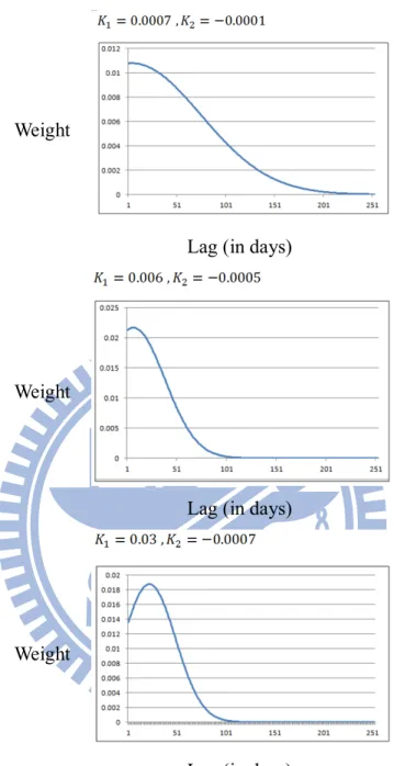
Figure 1: MIDAS Weight with Exponential Polynomial
Weight
Lag (in days)
Weight
Lag (in days)
Weight
Lag (in days)
The figure plots weight shapes of the mixed data sampling estimator. The weights are
calculated by substituting the estimated values of and into the weight equation (8). In the top panel, slowly declining weights are displayed. The middle panel shows rapidly
19
We clearly notice that the declining rate determines how many lags are included in
MIDAS regression Eq. (7). Once the weight form of ( ; , ) is specified, the lag length selection is totally data driven. When the function decays slowly, a large number of
observations need to be taken into consideration for the forecast of variances with small
measurement error. Conversely, a fast decay corresponds to using a small number of
observations with potentially large measurement error.
The second parameterization is also shown as follows:
( ; 1, 2) = ( ; , )
∑ ( ; , ) (9)
where ( , 1 , 2) = ( ) ( )
( ) ( ) , and Γ( 1) = ∫ . Eq. (9) is
based on Beta function so that we called it as “Beta Lag”. For example, we know that under
an assumption of = = 1 we have equal weights. As “Exponential Lag” case, the weight declining rate determines how many lags are included in the MIDAS regression. The
two specifications both have two important characteristics. First, they provide positive
coefficients, which is necessary for positive definiteness of estimated volatility. Second, they
sum up to one. In this paper, we use Exponential Lag as the specification, which is
theoretically more parsimonious. We choose the lagged period D as 22 days which is
corresponding to one month while comparing various predictors of conditional variance in
20 3.1.2. Volatility Predictors
Volatility predictors with various specifications also affect the risk premiums (see
Ghysels, Sinko, and Valkanov, 2007). In particular, some different ways are considered such
as: squared returns, absolute returns, return ranges, realized volatility, and realized power (the
sum of high frequency absolute returns). In general, we apply daily lagged squared risk
premiums and absolute range risk premiums as our volatility predictors. Here are MIDAS
general formulations:
ERP = + ∑ ( ; 1, 2) ERP + ε (10) ERP = + ∑ ( ; 1, 2) | ERP | + ε (11) where ERP is the lagged squared risk premium and | ERP | is the absolute risk premium in the MIDAS polynomial volatility predictor.
To estimate the parameters in MIDAS estimation, we use the variance estimator Eq. (7)
with the weight function Eq. (8) into the ICAPM relation Eq. (1) and estimate the parameters
μ and γ by maximizing the likelihood function. Assuming that the conditional distribution of return is normal:
ERP ~ N( + , ). (12) Because the true conditional distribution of returns could depart from normality, our
21
Using higher frequency returns at daily or weekly interval could improve the estimate of
because of the availability of additional data points. On the other hand, quarterly returns could
increase the efficiency of the estimator of because they are less volatile.
3.2 GARCH-in-Mean Estimation
In finance, the returns of a security may depend on its volatility. Engle et al. (1987) have
s study for three-month U.S. Treasury bills and six-month U.S. Treasury bills from 1960Q1 to
1984Q2. They claim that the expected return varies while the risk changes, therefore they take
varying conditional variance into GARCH consideration. That approach is known as
GARCH-in-mean model, where conditional mean is linearly related to the conditional
variance. (see Engle, Lilien and Robins, 1987). General GARCH-M models can be written as:
= + + (13) = + + (14) where and are constants. The parameter is called risk aversion parameter. The
formulation implies that there are serial correlations in the return series { } , the mean model. These serial correlations are introduced by those in the volatility process { }. As we can see, the GARCH-M model incorporates heteroskedasticity into the estimation procedure and
allows for direct estimate of time-varying risk premiums. Related to Merton’s ICAPM, some
22
steady variables except for the conditional variance, then these variables must be included in
the expected return equation (mean equation). The general formulation is as:
= + + (15)
where = − − . The squared error ε (regression error term) in the
variance estimator plays a role similar to the squared risk premium functions in MIDAS
approach.
3.3 Rolling Window Estimation
A moving window is commonly used with time series data to smooth out short-term
fluctuations and highlight longer-term trends or cycles. As an example of rolling window
approach, French, Schwert and Stambaugh (1987) use within-month daily squared returns to
forecast next month’s variance:
= ∑ (16)
where D is the number of days used in the variance estimator. They apply the autoregressive
moving average (ARMA) process for one-month rolling window estimator to model the
conditional variance. In the meanwhile, daily squared returns are multiplied by 22 to measure
the variance in monthly unit. Here we still choose the window size to be one month, or D = 22.
Besides its simplicity, the use of daily data has a number of advantages. First, as with MIDAS
23
Second, the stock market variance is very persistent (see Officer, 1973; Schwert, 1989), so the
realized variance on a given month ought to be a good forecast of next month’s variance.
Then we estimate the parameters μ and γ of risk-return tradeoff in Eq. (1) with maximum likelihood using the rolling window estimator Eq. (16) for the conditional variance.
Based on the literature of Ghysels, Santa-Clara and Valkanov (2005), they suggest the
window size should not be limited. A larger window size corresponding to a more than one
month, even up to six months, is used because the choice of lagged period has a greater
impact on the estimate of γ. In this paper, we choose fixed window size D = 22 to estimate the risk premium in Taiwan stock market.
24 4 Empirical Results
4.1 Data
Here we use the daily risk premium of Taiwan Stock Exchange Capitalization Weighted
Stock Index (TAIEX) compiled by Taiwan Stock Exchange Co., Ltd. (TWSE) in our
empirical test. The period is from January 2006 to December 2010, including 1246 daily
observations. Entire samples are all collected from TEJ (Taiwan Economic Journal). TEJ was
founded in April 1990 to provide quality, in-depth and extensive historical financial data and
information in the major financial markets in Asia. There is a definition about equity risk
premium in this paper: we use the difference, return rates of TSEC weighted index minus
two-year Taiwan treasury-bill rates, as a proxy to be explored, including various frequencies
such as daily, weekly and monthly data form. In the meantime, statistical software E-Views is
applied to analyze and compute some relevant data.
Table 1 shows the descriptive statistics about the sampled equity risk premium. We find
the mean for ERP is negative. That means on average there is no premium investors acquire in
the stock market during this period. Conversely, they even get some losses. Variances are used
in this table because of the relation between risk and return. Specifically, we focus on
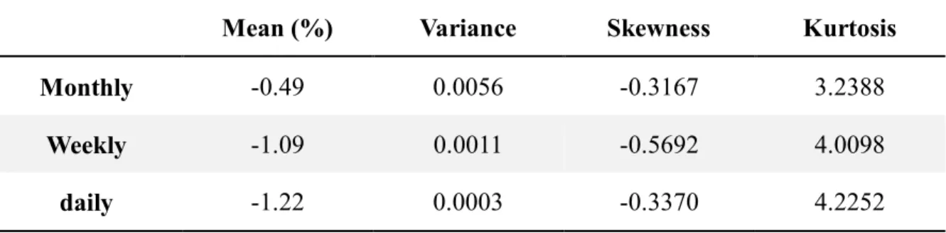
25 Table 1: Descriptive Statistics
Descriptive statistics of ERP with different sampling frequencies from 2006 to 2010, included are mean, variance, skewness, kurtosis. The number of samples for each frequencies is also reported in the table.
Mean (%) Variance Skewness Kurtosis
Monthly -0.49 0.0056 -0.3167 3.2388
Weekly -1.09 0.0011 -0.5692 4.0098
daily -1.22 0.0003 -0.3370 4.2252
4.2 MIDAS Estimation
This subsection is integrated from two parts. As we mentioned before, we decide to use
Exponential weight specification and apply the 30 days lags length. For first part, we apply
the suggestion under setting 1 = −0.01 and 2 = 0 (see Ghysels, Snata-Clara, and Valkanov, 2006b) as a benchmark. Then we compare it with other two cases: 1 = 0 and
2 = 0 (shown as equal weight) , 1 = −1 and 2 = 0 (considered as reasonable pattern). We plot the weights that the MIDAS estimator places of the first 22 lagged daily squared risk
premiums corresponding to one month in Figure 2. The top panel is case1, the middle panel is
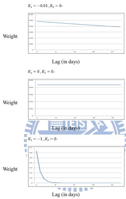
26 Figure 2: MIDAS Weight on Variables Predictors
Weight
Lag (in days)
Weight
Lag (in days)
Weight
Lag (in days)
The figure plots the estimated weights of conditional variance on the lagged daily squared risk premiums corresponding to one month. Three panels are representative of three different declining weight shapes respectively. We then use the weights to estimate related parameters by MIDAS approach.
27
Now we jointly estimate the parameters and by nonlinear least squares (NLS). In Table 2, we show three different weight polynomials and two various types of the volatility
predictors. We also explore the estimation results between MIDAS approach and rolling
window approach.
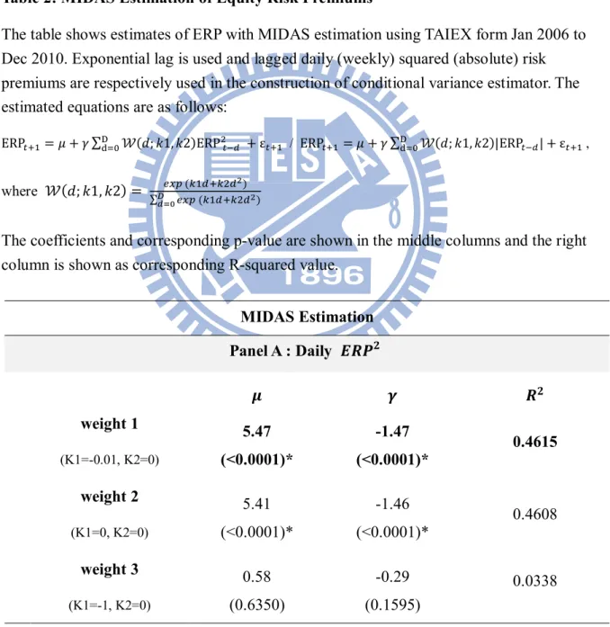
Table 2: MIDAS Estimation of Equity Risk Premiums
The table shows estimates of ERP with MIDAS estimation using TAIEX form Jan 2006 to Dec 2010. Exponential lag is used and lagged daily (weekly) squared (absolute) risk premiums are respectively used in the construction of conditional variance estimator. The estimated equations are as follows:
ERP = + ∑ ( ; 1, 2)ERP + ε / ERP = + ∑ ( ; 1, 2)|ERP | + ε ,
where ( ; 1, 2) = ∑ ( )
( )
The coefficients and corresponding p-value are shown in the middle columns and the right column is shown as corresponding R-squared value.
MIDAS Estimation Panel A : Daily weight 1 (K1=-0.01, K2=0) 5.47 (<0.0001)* -1.47 (<0.0001)* 0.4615 weight 2 (K1=0, K2=0) 5.41 (<0.0001)* -1.46 (<0.0001)* 0.4608 weight 3 (K1=-1, K2=0) 0.58 (0.6350) -0.29 (0.1595) 0.0338
28 Panel B : Weekly weight 1 (K1=-0.01, K2=0) 3.43 (0.0020)* -0.31 (<0.0001)* 0.3437 weight 2 (K1=0, K2=0) 3.35 (0.0025)* -0.30 (<0.0001)* 0.3379 weight 3 (K1=-1, K2=0) 2.50 (0.0194)* -0.03 (<0.0001)* 0.2795 Panel C : Daily | | weight 1 (K1=-0.01, K2=0) 9.50 (<0.0001)* -6.73 (<0.0001)* 0.4141 weight 2 (K1=0, K2=0) 9.38 (<0.0001)* -6.70 (<0.0001)* 0.4117 weight 3 (K1=-1, K2=0) 2.62 (0.1509) -2.09 (0.0472)* 0.0662 Panel D : Weekly | | weight 1 (K1=-0.01, K2=0) 7.12 (<0.0001)* -3.04 (<0.0001)* 0.3686 weight 2 (K1=0, K2=0) 6.96 (<0.0001)* -3.00 (<0.0001)* 0.3598 weight 3 (K1=-1, K2=0) 4.31 (0.0042)* -2.00 (0.0001)* 0.2266
29
This subsection presents the result of MIDAS approach based on the Merton’s ICAPM
model. We find the coefficients and are almost statistically significant. First, we start
from MIDAS estimation. In daily data, the estimated risk aversion coefficient is ranging
between -0.29 and -6.73. There is not a very small gap between the both sides. The risk
aversion absolute seems greater in daily data than in weekly data, and that means the degree
of risk aversion which can be tolerated by investors. In addition, we see that there are just
little differences between the weight 1 and weight 2 polynomials and R-square values
respectively. We also find such t-statistics of the corresponding estimated coefficient are
significant by judging from the p-values. We can conclude that volatility predictors of weight
1 and weight 2 are obviously better than weight 3. Actually, these results with polynomial
weight 3 are not explainable enough.
In weekly data, the estimated risk aversion coefficient is of -0.03 to -3.04 and the
difference is much closer. However, the result of weight 3 case becomes better because its
R-squares value is getting obviously higher, even over 20% extra. While mentioning to
R-square value, it is reports to quantify the explanatory power of the variance estimators in
predictive regressions for sampled premiums. To sum up, the estimation of daily risk premium
performs better than weekly risk premium because the significance of coefficients and
30
squared daily return volatility is also comparable to the result of absolute daily return
volatility. The risk aversion coefficients of weight 1 and 2 are -1.47and -1.46, and the model
explained variation levels are around 46.15% and 46.08% respectively. Basically both are
almost equivalent, but we still prefer to choose the estimation model under 1 = −0.01 and 2 = 0 with daily frequency. These results point to the importance of having a flexible functional form for the weights on past daily squared returns. Then we use out-sample to
measure forecasting errors in following subsection to make certain whether the estimation is
appropriate.
However, one thing important needs to be noticed. We all have negative magnitude of
risk aversion coefficients in above cases, no matter whether the squared risk premium or the
absolute risk premium is. It clearly points out that the tradeoff relation in our empirical study
is negative. These “negative” results are obviously corresponding to some previous classical
studies. Actually we think the results may depend on what the estimated method for the
conditional variance of returns is used. Campbell (1987) use generalized method moments
(GMM) to verify the relationship between expected stock returns and the conditional variance
of stock returns. The coefficient estimates of GMM for stock suggest that stocks have a higher
expected return when their conditional variance is low. Correspondingly, Nelson (1991) uses the GARCH method to estimate a model of the risk premium on the CRSP value-weighted
31
market index form 1962 to 1987. The outcome is shown as a statistically significantly
negative relation between both. In recent studies, Glosten et al. (1993) use the CRSP data and
find support of a negative relation between conditional expected monthly return and
conditional variance of monthly return, using the modified GARCH-M model. More related
interpretation we leave in Section 5.
4.3 GARCH-in-Mean Estimation
Before applying GARCH-M estimation, time series data should be processed by a kind of
unit tests and we find out the result shows significant rejections of null hypothesis which
mean the risk premium data is not autocorrelated. Then we directly use the data under
32
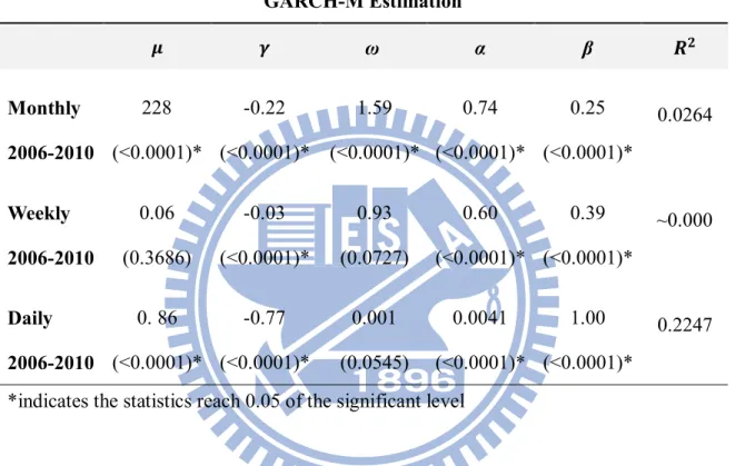
Table 3: GARCH-M Estimation of Equity Risk Premiums
The table shows estimates of ERP with GARCH-M estimation using TAIEX form Jan 2006 to Dec 2010. The estimated equations are as follows:
= + + , where = + + .
The coefficients and corresponding p-value are shown in the middle columns and the right column is shown as corresponding R-squared value.
GARCH-M Estimation ω α β Monthly 2006-2010 228 (<0.0001)* -0.22 (<0.0001)* 1.59 (<0.0001)* 0.74 (<0.0001)* 0.25 (<0.0001)* 0.0264 Weekly 2006-2010 0.06 (0.3686) -0.03 (<0.0001)* 0.93 (0.0727) 0.60 (<0.0001)* 0.39 (<0.0001)* ~0.000 Daily 2006-2010 0. 86 (<0.0001)* -0.77 (<0.0001)* 0.001 (0.0545) 0.0041 (<0.0001)* 1.00 (<0.0001)* 0.2247
*indicates the statistics reach 0.05 of the significant level
Table 3 shows the empirical results of GARCH(1,1)-M estimation of risk premium data
with different frequencies. The estimated coefficients are obtained by a sort of maximum
likelihood estimations, and we assuming error term is normally distributed. Compared
with other three different frequencies in GARCH-M estimation, the R-squared statistics with
daily frequency data is much better. In addition, the GARCH-M model with daily frequency
33
term. The risk aversion coefficient γ is around of -0.77 for the mean equation and the p-value of the corresponding estimated coefficient looks very significantly. Here we notice that the
risk aversion is still negative, consistent with the MIDAS estimation as we mentioned above.
Besides, under the GARCH-M approach the R-squared statistic is around of 22.47%,
lower than in the MIDAS approach which is shown as 46.15%. Take this for example, it is
because the MIDAS approach estimates two parameters rather than three as GARCH-M
model does and employs more observations to forecast market volatility under variance
equation. In generally speaking, traditional GARCH-M estimation outcome in explainable
range is not superior to the MIDAS approach.
4.4 Rolling Window Estimation
We discuss about the rolling window estimation with daily and weekly frequency data.
The results of rolling window approach are shown in Table 4. The estimate of is still
negative (around of -1.4), and the coefficient is very significant because the p-value is far
lower than the significant level. It is shown consistently under this situation with the MIDAS
estimation. Besides, R-square value is 46.08% of rolling window estimation, and almost as
same as the MIDAS estimation, 46.15%. They are so close but obviously we still recognize
that the daily frequency specification is better as a result of the higher R-squared value. The
34
it is a simple estimator of conditional variance with no parameters to be estimated. Besides its
simplicity, the use of daily data has some advantages: first, as with MIDAS approach, it can
increase the precision of the variance estimator. Second, the stock market variance is quite
persistent (see Officer, 1973; Schwert, 1989), so the realized variance on a given month ought
to be a good forecast of next month’s variance.
Table 4: Rolling Window Estimation of Equity Risk Premiums
The table shows estimates of ERP with rolling window estimation using TAIEX form Jan 2006 to Dec 2010. The estimated equations are as follows:
= + + , where = ∑
The coefficients and corresponding p-value are shown in the middle columns and corresponding R-squared values are shown in the right column.
Rolling Window Estimation
Daily 5.41 (<0.0001)* -1.40 (<0.0001)* 0.4608 Weekly 3.35 (0.0025)* -0.29 (<0.0001)* 0.3379
*indicates the statistics reach 0.05 of the significant level
4.5 Forecasting
Analysts are often interested in comparing the accuracy of competing forecasts, for a
35
competing models. Accordingly, a number for equal forecast accuracy have been developed.
After estimating as above, here we use out-sample data to compare the risk premium
forecasting errors. The purpose of forecasting is to understand whether these approaches
maintain consistent performances under out-sample by observing how much close is between
risk premium estimators and the realized data. The smaller the estimator error is, the better the
estimation performs. At first, we use in-sample data between Jan 2006 and Dec 2010 to
estimate the original parameters ( , ) as shown in Table 2, 3, 4. In general, percentage of in-sample observations to out-sample observations ratio is about 10% or 15% (see Ashley,
2003). Therefore, we decide to choose 12 months as our forecasting period.
Some literatures discuss the various approaches to forecast estimation errors, such as
mean error (ME), mean square error (MSE), root mean square error (RMSE), mean absolute
error (MAE) and mean absolute percent error (MAPE). In this paper, we apply RMSE and
MAE approaches to measure prediction level in various volatility estimation models.
4.5.1 Root Mean Square Error
The root mean square error (RMSE) (see Christiano, 1989) is a frequently used measure
of differences between an estimator and the values actually observed. The concept of RMSE
36
RMSE = ∑ ( − )
where is the realized volatility on day t , is the foracasted volatility on day t , N
denotes sampling days.
4.5.2 Mean Absolute Error
In practice, the mean absolute error (MAE) is to measure how close forecasts are to
eventual outcomes. The mean absolute error is given by: MAE = ∑ | |
4.5.3 Forecasting Results
For the reason we pay attention to the importance of out-sample forecasting is that it can
avoid the situations of over-fitting models or of abusing data-mining. Forecasting accuracy
comparison can help discriminate among competing models. Several recent studies have
examined the small-sample properties of some commonly used tests, too. In fact, we focus not
only on comparing with different models, but also on understanding the forecasting accuracy
37 Table 5: Results of Forecasting Error
The table shows the forecasting error results by using RMSE / MAE for out-sample.
Comparing Forecasts In-sample (60) Out-sample (12) MIDAS RMSE 5.4498 8.1490 MAE 4.3284 5.9583 GARCH-M RMSE 7.3795 5.5631 MAE 5.6129 5.5631 Rolling Window RMSE 5.4536 8.4781 MAE 4.3435 6.5689
All forecasting error unit is of percentage (%)
From Table 5, no matter whether RMSE or MAE estimation is used, obviously we find
that out-sample performance of GARCH-M estimation is quite good, which means the
smaller errors. However, errors of in-sample under GARCH-M estimation are the largest,
even up to 7.3795%, almost 1.7 times to the smallest one. On the other hand, we realize that
MIDAS and rolling window estimations are basically developed form similar concepts and
the forecasting results vary consistently and stably. Overall, forecasting errors in using
MIDAS is close to GARCH-M, which is almost of 0.4% in difference under MAE approach.
38
GARCH-M under MAE approach in out-sample. These approaches of forecasting error
sequentially ranked as GARCH-M, MIDAS and RW estimation from the smallest error to the
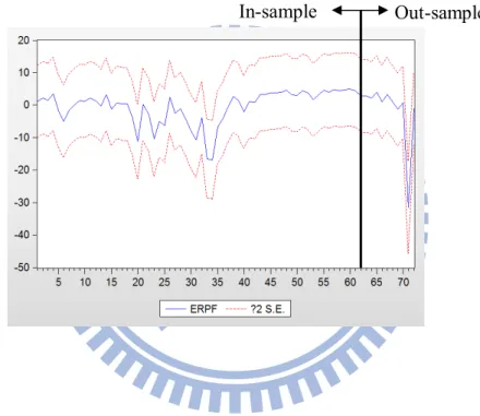
largest error. Figure 3 shows forecasting graph under MIDAS and Table 6 shows error
differences under MIDAS as follows.
Figure 3: Forecasting Graph with MIDAS Estimation
39 Table 6: Out-Sample Errors (2011.1 – 2011.12)
Period (year/month) Real ERP Forecasted ERP Error (%)
2011.1 1.3564 4.4178 3.0614 2011.2 -6.657 2.8815 9.5385 2011.3 0.1501 2.9229 2.7728 2011.4 2.9379 4.051 1.1131 2011.5 -1.0121 4.004 5.0161 2011.6 -4.5668 2.9358 7.5026 2011.7 -0.9472 3.4425 4.3897 2011.8 -11.2543 -3.1977 8.0566 2011.9 -7.4062 -1.4198 5.9864 2011.10 4.2511 2.7699 1.4812 2011.11 -9.7889 -31.7794 21.9905 2011.12 1.6078 1.0167 0.5911 All forecasting error unit is of percentage (%)
40 5 Conclusion
This paper take a new look at Merton’s ICAPM, focus on the trade-off between
conditional variance and conditional mean of the stock market return. We show the existence
of a time-varying risk premium in Taiwan stock market by introducing mixed data sampling
model estimation. Our results are more conclusive because MIDAS estimation confirms the
weighted polynomial with different sampling frequencies performs pretty good. Not the same
as with previous studies, added power obtained from the new MIDAS estimator actually
makes risk premium estimation more flexible.
According to the previous empirical results, conclusions of this study are as follows:
1) The tradeoff between risk and return has long been an important topic in asset valuation
research. Most of this research examine the tradeoff among different securities within a
given time period. We find the common evidence of a negative relation between risk and
return in Taiwan stock market within these years. In fact, we think that what types of
model are used to assume conditional variance of returns as a research framework is
highly relevant to the issue of risk-return relation regardless of positive relation or
negative relation. However, sometimes the models we used cannot completely capture
41
Black (1976) and Christic (1982) propose financial leverage effect for an
examination of the risk-return tradeoff with asymmetric variance effect. After that,
Campbell and Hentschel (1992) propose volatility feedback effect to explain the same
situations. Most empirical studies show that negative relation between risk and return
might be attributed to asymmetric effects in the conditional variance. Moreover, the type
of relevance is mostly confined by model assumptions which indeed affect these empirical
results.
In addition to asymmetric effect, many different approaches for setting risk as a
proxy variable could also affect the empirical results, especially for risk-return tradeoff.
Moreover, the financial tsunami brings about some potential phenomenon such as
increasing difficulty in predicting expected returns and conditional variances. Meanwhile,
it also indeed related to the sampling period we selected. Although we acquire negative
relation about risk-return tradeoff, which is opposed to some previous research, we still
show some advantages in MIDAS estimation as follows.
2) Comparing with the rolling window and GARCH-M estimation, we conclude that MIDAS
estimation is better and more suitable. As the model explained variation power, 46.15% of
MIDAS is larger than 46.07% of rolling window, also greater than 22.47% of GARCH-M.
42
because it is a simple estimator of conditional variance with no parameters to be estimated.
Except for explained variation power, these estimation coefficients are very statistically
significant because of p-values are below significance level. That means the MIDAS
estimation is indeed a well-performed model.
3) By using MIDAS approach, this estimator is behalf of a weight average of past daily
squared returns with flexible functions. MIDAS estimator is not only the superior
estimator because it can be appropriately explained by past risk premiums, but also a
better forecaster in the stock market than rolling window estimators. Last but not the least,
after experiencing investigations of the MIDAS specifications for various volatility
predictors, we obtain that higher frequency predictor such as daily squared return provides
greater results.
The empirical results are statistically significant, at the same time, the forecasting
performance of MIDAS is also reasonable. We still have interests to use MIDAS to process
how these different and jointly estimated weights of volatility predictor work. Next, we
explore the parameters 1 and 2 more deeply. Our purpose is to directly and jointly estimate the parameters 1 , 2 , μ , γ of Eq. (6) and (7) by nonlinear least error approach. Owing to the smaller the conditional variance is, the smaller the estimated forecasting error is.
43
Therefore we apply MAE and RMSE forecasting error approaches, and then make certain that
the values of MAE and RMSE are both minimum. Our estimated algorithm is as follows,
which is based on rules of minimum error. Take MAE for example, our main purpose is to
minimize the value of ∑ | | , which is under restrains of = ̂ + ( ) ,
and = ∑ ( )
∑ ( ) .
After jointly nonlinear least error calculation with the same period, our results are shown
in Table 7.
Table 7: Errors of Jointly Nonlinear Least Calculation Forecasting Estimation Minimum Error (%) 0.0096 (RMSE) -0.3163 -0.0503 1.2346 -18.3336 0.0020 0.0564 (MAE) 0.0105 -0.0002 1.2346 -18.3336 ~0.000
*indicates the statistics reach 0.05 of the significant level All forecasting error unit is of percentage (%)
We find that the outcome is not good enough while comparing with previous results
44
significant because the p-values are not below the significance level 0.05. Moreover, the
explanatory power is also abnormally low so that we cannot verify this case to be well. Here
is a trivial implication that the suggestion of setting and as some specific values (see
Ghysels et al., 2006) improves the outcomes of MIDAS estimation better. As for the reasons
why the effects of estimated weight polynomial parameter such as are not relatively
45
6 References
Andreou, E., Ghysels, E. and Kourtellos, A., “Regression Models with Mixed Sampling Frequencies”, Journal of Econometrics, 158, pp. 246-261, 2010.
Backus, D. K. and Gregory A. W., “Theoretical Relations between Risk Premiums and Conditional Variances”, Journal of Business & Economic Statistics, 11, pp. 177-185, 1993.
Bansala, R. and Lundbladb, C., “Market Efficiency, Asset Returns, and the Size of the Risk Premium in Global Equity Markets”, Journal of Econometrics, 109, pp. 195-237, 2002.
Bollerslev, T., “Generalized Autoregressive Conditional Heeteroskedasticity”, Journal of Econometrics, 31, pp. 307-327, 1986.
Bollerslev, T. and Wooldridge J. M., “Quasi-Maxmimum Likelihood Estimation and Inference in Dynamic Models with Time-Varying Covariances”, Econometric Reviews, 11, pp. 143-172, 1992.
Braun, P. A., Nelson, D. B. and Sunier, A. M., ”Good News, Bad News, Volatility, and Betas”, Journal of Finance, 50, pp. 1575-1603, 1995.
Campbell, J. Y., “Stock Returns and the Term Structure”, Journal of Financial Economics, 18, pp. 373-399, 1987.
Campbell, J. Y. and Hentschel, L., “No News is Good News: An Asymmetric Model of
Changing Volatility in Stock Returns”, Journal of Financial Economics, 31, pp. 281-318, 1992.
Chen, P. and Ibbotson, R. G., The Supply of Stock Market Returns, Yale School of Management, Connecticut, 2001.
Chou, R. Y., “Volatility Persistence and Stock Valuations: Some Empirical Evidence Using Garch”, Journal of Applied Econometrics, 3, pp. 279-294, 1988.
Clements, M. P. and Galvao, A. B., Macroeconomic Forecasting with Mixed Frequencies Data: Forecasting US Output Growth and Inflation, University of Warwick, Coventry, 2006.
Cornell, B., The Equity Risk Premium: The Long-Run Future of the Stock Market, John Wiley & Sons, New York, 1999.
46
Damodaran, A., Equity Risk Premiums (ERP): Determinants, Estimation and Implication, Stern School of Business, New York, 2010.
Enders, W., Applied Econometric Time Series, John Wiley & Sons, New York, 2010.
Engle, R. F., Lilien, D. M. and Robins, R. P., “Estimating Time Varying Risk Premia in the Term Structure: the Arch-M Model”, Econometrica, 55, pp. 391-407, 1987.
French, K. R., Schwert, G. W. and Stambaugh, R. F., ”Expected Stock Returns and Volatility”, Journal of Financial Economics, 19, pp. 3-29, 1987.
Ghysels, E., Sinko, A. and Valkanov, R., “MIDAS Regressions: Further Results and New Directions”, Econometric Reviews, 26, pp. 53-90, 2007.
Ghysels, E., Santa-Clara, P. and Valkanov, R., The MIDAS Touch: Mixed Data Sampling Regression Models, Anderson Graduate School of Management, California, 2004.
Ghysels, E., Santa-Clara, P. and Valkanov, R., “There Is a Risk-Return Tradeoff After All”, Journal of Financial Economics, 76, pp. 509-548, 2005.
Ghysels, E., Santa-Clara, P. and Valkanov, R., “Predicting Volatility: Getting the Most out of Return Data Sampled at Different Frequencies”, Journal of Econometrics, 131, pp. 59-95, 2006.
Glosten, L. R., Jaganathan, R. and Runkle, D. E., “On the Relation between the Expected Value and the Volatility of the Nominal Excess Return on Stocks”, The Journal of Finance, 48, pp. 1779-1801, 1993.
Goetzmann, W. N. and Ibbotson, R. G., History and the Equity Premium, Yale School of Management, Connecticut, 2005.
Grahama, J. R. and Harvey, C. R., “The Long-Run Equity Risk Premium”, Finance Research Letters, 2, pp. 185–194, 2005.
Hansen, P. R. and Lunde, A., “A Forecast Comparison of Volatility Models: Does Anything Beat a GARCH(1,1)?”, Journal of Applied Econometrics, 20, pp. 873-889, 2005.
Hsu, C. H., “Estimating Risk Premiums of Taiwan's U.S. Dollar Forward Rates Using MIDAS”, National Chiao Tung University, Master's Thesis, 2008.
Hyndmana, R. J. and Koehlerb, A. B., “Another Look at Measures of Forecast Accuracy”, International Journal of Forecasting, 22, pp. 679–688, 2006.
47
Financial Econometrics, 5, pp. 560–590, 2007.
Koutmos, G., Knif, J. and Philippatos, G. C., “Modeling Common Volatility Characteristics and Dynamic Risk Premia in European Equity Markets”, The Quarterly Review of Economics and Finance, 48, pp. 567-578, 2008.
Leon, A., Nave, J. M. and Rubio, G., “The Relationship between Risk and Expected Return in Europe”, Journal of Banking & Finance, 31, pp. 495-512, 2007.
Ludvigson, S. C. and Ng, S., “The Empirical Risk-Return Relation: A Factor Analysis Approach”, Journal of Financial Economics, 83, pp. 171-222, 2007.
Lundblad, C., “The Risk Return Tradeoff in the Long-Run: 1836-2003”, Journal of Financial Economics, 85, pp. 123-150, 2007.
Merton, R. C., “An Intertemporal Capital Asset Pricing Model”, Econometrica, 41, pp. 867-887, 1973.
Nelson, D. B., “Conditional Heteroskedasticity in Asset Returns: A New Approach”, Econometrica, 59, pp. 347-370, 1991.
Sentana, E., “Quadratic ARCH Models”, Review of Economic Studies, 62, pp. 639-661, 1995.
Seruggs, J. T., “Resolving the Puzzling Intertemporal Relation between the Market Risk Premium and Conditional Market Variance: A Two-Factor Approach”, The Journal of Finance, 53, pp. 575-603, 1998.
Tsay, R. S., Analysis of Financial Time Series, John Wiley & Sons, New Jersey, 2010.
丁純蘭,「應用 MIDAS 模型之避險效果分析」,國立交通大學,碩士論文,民國九十六 年。
李美樺,「以橫斷面跨期資本資產定架模型衡量台灣股市報酬與風險之動態關係」,銘傳 大學,碩士論文,民國九十六年。