受限背填土對主動土壓力之影響

(1)

國立交通大學

土木工程學系碩士班

碩士論文

受限背填土

受限背填土對主動土壓力之影響

對主動土壓力之影響

Effects of Constrained Backfill on Active Earth Pressure

研

研究

究

究生

生

生 : 陳威廷

陳威廷

指導教授

指導教授 : 方永壽

方永壽

方永壽博士

博士

中

中華

華

華民

民

民國

國

國九十九

九十九年

九十九

年

年七

年

七

七月

七

月

(2)

受限背填土

受限背填土對主動土壓力之影響

對主動土壓力之影響

Effects of Constrained Backfill on Active Earth

Pressure

研究生: 陳威廷

Student：Wei-Ting Chen

指導教授：方永壽博士

Advisor：Dr. Yung-Show Fang

國立交通大學土木工程學系碩士班

碩士論文

A Thesis

Submitted to the Department of Civil Engineering

College of Engineering

National Chiao Tung University

in Partial Fulfillment of the Requirements

for the Degree of

Master of Engineering

in Civil Engineering

July, 2010

Hsinchu, Taiwan, Republic of China

(3)

受限背填土對主動土壓力之影響

研究生 : 陳威廷指導教授 : 方永壽博士

國立交通大學土木工程學系碩士班

摘要

本研究探討受限背填土對主動土壓力之影響。本研究利用國立交通大學模型擋土牆設備來探討受限背填土作用在擋土牆上的主動土壓力。本研究以氣乾渥太華砂作為回填土，相對密度 Dr = 36%，回填土高 0.5 公尺。為了模擬束制背填土的岩層介面，本研究設計並建造一片鋼製傾斜界面板及其支撐系統。本研究兩個重要參數為界面板與擋土牆底之水平間距 b 及界面板傾角β。試驗結果顯示，以空中霣降法填入土槽之背填土密度均勻，且背填土之相對密度不受界面板位置與傾角影響。當界面板遠離擋土牆(b/H = 4.0)，量測到的水平主動土壓力與 Coulomb 解符合良好。當 b/H = 1.0，量測到的主動土壓力接近於 Coulomb 解，於此狀況界面板對主動土壓力沒有明顯的影響。當界面板逐漸接近擋土牆時(b/H 減小)，界面板逐漸侵入主動土楔，造成主動土楔無法完全發展，且牆後填土量逐漸減少，隨著逐漸減小的水平距離 b，和逐漸增大的界面板傾斜角度β，主動土壓力逐漸下降。於β = 90°(牆面垂直)且 b/H < 1.0 狀況，量測到的主動土壓力小於 Coulomb 解，靠近牆面之垂直界面板對於主動土壓力的影響相當明顯。於 b/H = 0.3、0.5、0.7 及 1.0，主動土壓力合力作用點的位置大約都在距牆底 H/3 處。當傾斜岩石介面逐漸接近擋土牆，依據 Coulomb 理論所求之擋土牆抗滑動之安全係數及抗傾覆之安全係數增大。關鍵字關鍵字關鍵字關鍵字：：：主動土壓力、受限背填土、土壓力、模型試驗、擋土牆、砂：

(4)

Effects of Constrained Backfill on Active Earth Pressure

Student : Wei-Ting Chen Advisor : Dr. Yung-Show Fang

Department of Civil Engineering National Chiao Tung University

Abstract

This thesis investigates the effects of constrained backfill on active earth pressure. The instrumented model retaining wall facilities at National Chiao Tung University was used to study the active earth pressure on retaining wall with constrained backfill. Loose Ottawa sand with the relative density Dr = 36% was used as backfill material. The height of backfill H was 0.5 m. To simulate an inclined rock face, a steel interface plate and its supporting system were designed and constructed. Two main parameters considered were rock face inclination angle β and the horizontal spacing b between the rock face and the wall base. The backfill in the soil bin was prepared by air-pluviated method. Test results show the distribution relative density in the soil bin is uniform and independent of the interface plate inclination and location. With a faraway interface plate (b/H = 4.0), the measured active pressure distribution was in good agreement with Coulomb’s solution. When the vertical boundary was relatively far from the wall face, the measured stress was not strongly affected by the existence of the vertical plate. With the approaching of the interface plate (b/H ratio decreasing), the plate intruded the active soil wedge, so that the active soil wedge behind the wall can not develop fully. The active earth pressure coefficient Ka,h decreased with decreasing wall-plate spacing b. Coefficient Ka,h decreased with decreasing plate inclination angle β. For β = 90° (vertical plate) and b/H < 1.0, the measured active pressure was less than Coulomb’s solution. Coulomb’s solution is the upper bound for all experimental Ka,h values based on

(5)

factor of safety against sliding for the retaining wall. Under the aspect ratio b/H = 0.3, 0.5, 0.7, and 1.0, the point of application of the active soil thrust was located at about H/3 above the wall base. The evaluation of the factors of safety against sliding and overturning with Coulomb’s solution would be on safe side.

Keywords: Active pressure; Constrained backfill; Earth pressure; Model test;

(6)

Acknowledgements

The author wishes to give his sincere appreciation to his advisor, Dr. Yung-Show Fang for his enthusiastic advice and continuous encouragement in the past two years. If there is not the guidance from him, the thesis can not be accomplished.

Very special thanks are extended to Dr. Yi-Wen Pan, Dr. Jhih-Jhong Liao, Dr. An-Bin Huang, Dr. Shen-Yu Shan and Dr. Chih-Ping Lin for their teaching and valuable suggestions. In addition, the author also felt a great gratitude to the members of his supervisory committee, Dr. Mei-Ling Lin andDr. Tao-Wei Feng for their suggestions and discussions.

The author must extend his gratitude to Dr. Tsang-Jiang Chen, Mr. Kuo-Hua Li, Mr. Hao-Chen Chang, Mr. Po-Shou Chen, Mr. Sheng-Feng Huang and Miss Yi-Jhen Jiang for their support and encouragement. Appreciation is extended to all my friends and classmates, especially for Mr. Cho-Min Lin, Miss Yu-Fen Hsu, Mr. Kuan-Yu Chen, Mr. Ting-Yuen Huang and Mr. Min-Yi Huang for their encouragement and assistance.

Finally, the author would dedicate this thesis to his grandmother, parents and brother for their continuing encouragement and moral support.

(7)

List of Tables

Table 2.1. Comparison of experimental and theoretical values………...54 Table 2.2. Wall displacements required to reach an active state………..55 Table 6.1 Test Program……….56

(11)

List of Figures

Fig. 1.1. Fig. 1.1. Retaining walls with constrained backfill 57

Fig. 1.2. Cylindrical silo filled with granular material 58

Fig. 1.3. Model test for b = 150 mm 59

Fig. 1.7. Model test for b = 2,000 mm 63

Fig. 2.1. Coulomb’s theory of active earth pressure 64

Fig. 2.2. Coulomb’s active pressure determination 65

Fig. 2.3. Rankine’s theory of active earth pressure 65

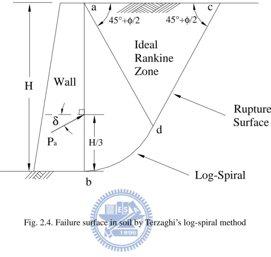
Fig. 2.4. Failure surface in soil by Terzaghi’s log-spiral method 66 Fig. 2.5. Evaluation of active earth pressure by trial wedge method 67

Fig. 2.6 Stability of soil mass abd1f1 68

Fig. 2.7 Active earth pressure determination with Terzaghi’s log-sprial failure surfaces

69

Fig. 2.8. Fascia retaining wall of backfill width B and wall friction F 70

Fig. 2.9. Horizontal element of backfill material 71

Fig.. 2.10. Distribution of soil pressure against fascia walls due to partial support from wall friction F

72

Fig. 2.11. University of Manchester model retaining wall 73

Fig. 2.12. Earth pressure with wall movement 74

Fig. 2.13. Failure surfaces 75

Fig. 2.14. Distributions of horizontal earth pressure at different wall displacement 76 Fig. 2.15. Change of normalized lateral pressure with translation wall

displacement

77

Fig. 2.16. Coefficient of horizontal active thrust as a function of soil density 78

(12)

Fig. 2.18. Different interface inclinations for b = 50 mm 80

Fig. 2.19. Different interface inclinations for b = 100 mm 81

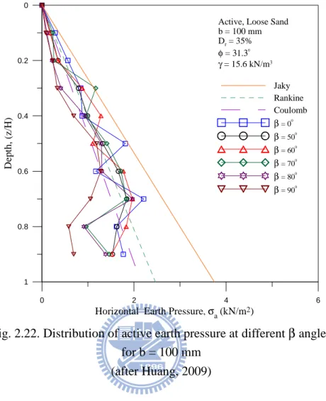
Fig. 2.20. Distribution of active earth pressure at different β angles for b = 0 82 Fig. 2.21. Distribution of active earth pressure at different β angles for b = 50 mm 82 Fig. 2.22. Distribution of active earth pressure at different β angles for

b = 100 mm

83

Fig. 2.23. Active earth pressure coefficient Ka,h versus interface inclination angle β

84

Fig. 2.24. Point of application of active soil thrust versus interface inclination angle β

85

Fig. 2.25 Schematic representation of retaining wall near rock face 86

Fig. 2.26. Model retaining wall 87

Fig. 2.27. Distribution of K’awith z/b from silo pressure equation 88

Fig. 2.28. Typical geometry: (a) analyzed (b) notation 89

Fig. 2.29. Predictions by ReSSA versus centrifugal test results for φ = 36° and m = ∞

90

Fig. 2.30. Analysis results 90

Fig. 2.31. Forces acting on wall face, wedge angles, and horizontal force coefficients for fill φ’ = 30°

91

Fig. 2.32. Illustration of the simulated case 92

Fig. 2.33. Finite element (a) meshes for at-rest case and (b) model for active case 93 Fig. 2.34. Normalized earth pressure coefficient profiles along the wall face for

(a) at-rest and (b) active case

94

Fig. 2.35. Normalized equivalent earth pressure coefficients for (a)at-rest and (b) active case

95

Fig. 2.36. Typical geometry of backfill zone behind a retaining wall used in this study

96

Fig. 2.37. The finite element mesh for a retaining wall with limited backfill space 96

(13)

Fig. 2.38. Distribution of earth pressures with the depth at various wall displacements for walls in translation (T mode)

97

Fig. 2.39. Variation of the coefficient of active earth pressures

(Ka(Computed)/Ka(Coulomb)) with the inclination of rock faces at various fill widths (b) for walls undergoing translation

98

Fig. 2.40. Variation of the location of resultant (h/H) of active earth pressures with the inclination of rock faces at various fill widths (b) for walls undergoing translation (T mode)

99

Fig. 2.41. Definition of plane strain state-of-stress 100

Fig. 3.1. NCTU Model Retaining-Wall Facility 101

Fig. 3.2. NCTU model retaining wall 102

Fig. 3.3. Displacement transducer (Kyowa DT-20D) 102

Fig. 3.4. Locations of pressure transducers on NCTU model wall 103

Fig. 3.5. Locations of pressure transducers on model wall 104

Fig. 3.6. Soil pressure transducer (Kyowa PGM-0.2KG) 104

Fig. 3.7. Plastic-sheet on each sidewall 105

Fig. 3.8. Picture of Data acquisition system 106

Fig. 4.1. NCTU model retaining wall with inclined interface plate 107

Fig. 4.2. Steel interface plate 108

Fig. 4.3. Steel interface plate (picture) 109

Fig. 4.4 Top-view of model wall 110

Fig. 4.5. NCTU model retaining wall with interface plate supports 111

Fig. 4.6. Top supporting beam 112

Fig. 4.7. Steel interface plate and top supporting beam 113

Fig. 4.8. Base supporting block 114

Fig. 4.9. Base supporting boards 116

Fig. 5.1. Grain size distribution of Ottawa sand 117

Fig. 5.2. Shear box of direct shear test device 118

(14)

Fig. 5.4. Direct shear test to determinate wall friction 120 Fig. 5.5. Relationship between unit weight γ and wall friction angle δw 121

Fig. 5.6. Plastic-sheet lubrication layers on side walls 122

Fig. 5.7. Schematic diagram of sliding block test 123

Fig. 5.8 Sliding block test apparatus 124

Fig. 5.9 Variation of side-wall friction angle with normal stress 125 Fig. 5.10. Direct shear test to determine interface friction angle 126 Fig. 5.11. Relationship between unit weight γ and interface plate friction angle δi 127 Fig. 5.12. Relationship friction angle δ and soil unit weight γ 128

Fig. 5.13. Soil hopper 129

Fig. 5.14. Pluviation of Ottawa sand into soil bin 130

Fig. 5.15. Relationship between relation density and drop height 131

Fig. 5.16. Soil-density control cup 132

Fig. 5.17. Soil-density cup 133

Fig. 5.18. Locations of density cups for b = 150 mm and β = 90° 134 Fig. 5.19. Locations of density cups for b = 250 mm and β = 90° 135 Fig. 5.20. Locations of density cups for b = 350 mm and β = 90° 136 Fig. 5.21. Locations of density cups for b = 500 mm and β = 90° 137 Fig. 5.22. Locations of density cups for b = 150 mm and β = 80° 138 Fig. 5.23. Locations of density cups for b = 150 mm and β = 70° 139 Fig. 5.24. Locations of density cups for b = 150 mm and β = 60° 140

Fig. 5.25 Distribution of relative density 141

Fig. 6.1. Model wall test with faraway interface plate (b = 2,000 mm and β = 90°)142 Fig. 6.2. Distribution of horizontal earth pressure for b = 2,000 mm and β = 90°

(Test 0119-1)

144

Fig. 6.3. Distribution of horizontal earth pressure for b = 2,000 mm and β = 90°

(15)

Fig. 6.4 Earth pressure coefficient Kh versus wall movement for b = 2,000 mm and β = 90°

145

Fig. 6.5. Location of total thrust application for b = 2,000 mm and β = 90° 145 Fig. 6.6. Model wall test with interface spacing b = 150 mm and β = 900 146 Fig. 6.7. Distribution of horizontal earth pressure for b = 150 mm and β = 900

(Test 0305-1)

148

Fig. 6.8. Distribution of horizontal earth pressure for b = 150 mm and β = 900 (Test 0503-4)

148

Fig. 6.9. Model wall test with interface spacing b = 150 mm and β = 800 149 Fig. 6.10 Distribution of horizontal earth pressure for b = 150 mm and β = 800

(Test 0315-3)

151

Fig. 6.11 Distribution of horizontal earth pressure for b = 150 mm and β = 800 (Test 0316-2)

151

Fig. 6.12. Model wall test with interface spacing b = 150 mm and β = 70 152 Fig. 6.13. Distribution of horizontal earth pressure for b = 150 mm and β = 700

(Test 0413-1)

154

(Test 0420-3)

157

Fig. 6.18. Earth pressure coefficient Kh versus wall movement for b = 150 mm and β = 90°

158

(16)

159

Fig. 6.22. Location of total soil thrust for b = 150 mm and β = 900 160 Fig. 6.23. Location of total soil thrust for b = 150 mm and β = 800 160 Fig. 6.24. Location of total soil thrust for b = 150 mm and β = 700 161 Fig. 6.25. Location of total soil thrust for b = 150 mm and β = 600 161 Fig. 6.26. Model wall test with interface spacing b = 250 mm and β = 900 162 Fig. 6.27. Distribution of horizontal earth pressure for b = 250 mm and β = 900

(Test 0322-3)

164

(Test 0518-3)

167

(Test 0524-1)

170

Fig. 6.35. Earth pressure coefficient Kh versus wall movement for b = 250 mm and β = 900

171

172

(17)

Fig. 6.40. Location of total soil thrust for b = 250 mm and β = 700 174 Fig. 6.41. Model wall test with interface spacing b = 350 mm and β = 900 175 Fig. 6.42. Distribution of horizontal earth pressure for b = 350 mm and β = 900

(Test 0330-2)

177

(Test 0525-1)

180

181

Fig. 6.49. Location of total thrust application for b = 350 mm and β = 900 182 Fig. 6.50. Location of total thrust application for b = 350 mm and β = 800 182 Fig. 6.51. Model wall test with interface spacing b = 500 mm and β = 900 183 Fig. 6.52. Distribution of horizontal earth pressure for b = 500 mmand β = 900

(Test 0412-2)

185

Fig. 6.53. Distribution of horizontal earth pressure for b = 500 mmand β = 900 (Test 0412-3)

185

186

Fig. 6.55. Location of total thrust application for b = 500 mm and β = 900 186 Fig. 6.56. Distribution of active earth pressure at different interface inclination

angle β for b = 150 mm

187

Fig. 6.57 Distribution of active earth pressure at different interface inclination angle β for b = 250 mm

(18)

Fig. 6.58. Distribution of active earth pressure at different interface inclination angle β for b = 350 mm

188

Fig. 6.59. Distribution of active earth pressure for b = 500 mm 188 Fig. 6.60. Variation of earth pressure coefficient Kh with wall movement for

b = 150 mm

189

Fig. 6.61. Variation of earth pressure coefficient Kh with wall movement for b = 250 mm

189

190

Fig. 6.64. Variation of total thrust location with wall movement for b = 150 mm 191 Fig. 6.65. Variation of total thrust location with wall movement for b = 250 mm 191 Fig. 6.66. Variation of total thrust location with wall movement for b = 350 mm 192 Fig. 6.67. Variation of total thrust location with wall movement for b = 500 mm 192 Fig. 6.68. Active earth pressure coefficient Ka,h versus constrained backfill aspect

ratio b/H

193

Fig. 6.69. Normalized active earth pressure coefficient with aspect ratio b/H 194 Fig. 6.70. Point of application of active soil thrust versus aspect ratio b/H 195

Fig. 6.71. Cylindrical silo filled with granular material 196

Fig. 6.72. Distribution of active earth pressure at different backfill aspect ratio b/H for β = 90°

196

Fig. 6.73 Variation of earth pressure coefficient Kh with wall movement for β = 90°

197

Fig. 6.74. Variation of soil thrust location with wall movement for β = 90° 197 Fig. 6.75. Comparison of the distribution of active earth pressures 198 Fig. 6.76 Observed backfill displacement for b = 500 mm and β = 90° for

(a) S = 0 (b) S/H =0.04

(19)

Fig. 6.77 Accumulated displacement for b = 500 mm and β = 90°for S = 20 mm (S/H = 0.04)

200

Fig. 6.78 Observed backfill displacement for b = 150 mm and β = 90°for (a) S = 0 and (b) S = 20 mm (S/H =0.04)

201

Fig. 6.79 Accumulated displacement for b = 150 mm and β = 90°for S = 20 mm (S/H = 0.04)

202

(20)

List of Symbols

Cu =Uniformity Coefficient

b =Distance between Interface Plate and Model Wall Dr =Relative Density

D10 =Diameter of Ottawa Sand whose Percent finer is 10% D60 =Diameter of Ottawa Sand whose Percent finer is 60% emax =Maximum Void Ratio of Soil

emin =Minimum Void Ratio of Soil F =Force

Gs =Specific Gravity of Soil h =Location of Total Thrust

(h/H)a =Point of Application of Active Soil Thrust H =Effective Wall Height

i =Slop of Ground Surface behind Wall Ko =Coefficient of Earth Pressure At-Rest Ka =Coefficient of Active Earth Pressure Kh =Coefficient of Horizontal Earth Pressure

Ka,h =Coefficient of Horizontal Active Earth Pressure Pa =Total Active Force

β =Angle of Inclination Rock Face S =Wall Displacement

T =Translation

z =Depth from Surface σh =Horizontal Earth Pressure σ =Normal Stress

(21)

γ =Unit Weight of Soil

φ =Angle of Internal Friction of Soil δi =Angle of Interface Friction δsw =Angle of Side-Wall Friction

(22)

Chapter 1 Introduction

This thesis studies the effects of a constrained soil backfill on the active earth pressure against a retaining wall as shown in Fig. 1.1. In the figure, an inclined rock face is near the retaining wall. The backfill is constrained and the active soil failure wedge behind the wall can not develop fully. Under such a condition, the active earth pressure may be different from Coulomb’s and Rankine’s theories. In this study, experiments were conducted to investigate the distribution of active earth pressure as a function of the inclination angle β and the horizontal spacing b of the inclined rock face.

1.1 Objectives of Study

The calculation of forces exerted by soil against structures was one of the oldest problems in soil mechanics. The most widely accepted theories to estimate earth pressure are those of Coulomb and Rankine. For the gravity wall shown in Fig. 1.1, the Rankine active soil wedge is bounded by the wall and the failure plane with the inclination angle of 45° + φ/2 with the horizontal.

If the retaining wall is constructed adjacent to an existence stable face such as a stiff rock face near the retaining wall shown in Fig. 1.1, the stiff rock face might intrude the active soil wedge as the wall moves away from the backfill. In this case, can the Coulomb and Rankine theories be used to estimate the active earth pressure on the wall with constrained backfill? Would the distribution of active earth pressure still be linear with depth? To correctly calculate the factor of safety against sliding and overturning of the wall, it is necessary for the designer to understand how would the nearby rock face influence the active earth pressure. In Fig. 1.1, the horizontal

(23)

the inclination angle of the rock face with the horizontal is expressed as β.

Valuable studies associated with earth pressure on retaining walls with constrained backfill had been conducted. Based on the arching theory, Spangler and Handy (1984) developed a theoretical equation for calculating the lateral earth pressure acting on the wall of a silo. The granular particles in the silo were constrained by the vertical silo walls. Based on the limit equilibrium method and the computer program ReSSA 2.0, Leshchinsky et al. (2004) numerically investigated the lateral earth pressure on a Mechanically-Stabilized-Earth wall with constrained fill. Lawson and Yee (2005) used the limit equilibrium method to numerically investigate the lateral earth pressure acting on retaining walls with constrained reinforced fill. Yang and Liu (2007) conducted finite element analysis to study the earth pressure for narrow retaining. Fan and Fang (2009) used the non-linear finite element program PLAXIS (PLAXIS BV, 2002) to investigate the earth pressure against a rigid wall close to an inclined rock face. Huang (2009) used the model retaining wall facilities at National Chiao Tung University to investigate the active earth pressure on retaining walls near an inclined rock face.

Fig. 1.2 shows a cylindrical storage silo filled with granular material. It is important for designer to know how much lateral pressure is acting on the inside of silo walls. The silo wall deforms under the lateral pressure due to the granular. Due to symmetry, the center axis of the silo remains at-rest, which is similar to the vertical rock-face nearby. The granular material behind the deformable silo wall was restrained by the central axis of the silo. In this study, the lateral pressure in silo is discussed.

1.2 Research Outline

The National Chiao Tung University (NCTU) model retaining wall facility was modified to investigate the effects of a constrained backfill on the active earth

(24)

pressure. As shown in Fig. 1.1, two main parameters considered were the horizontal spacing b and the inclination angle β of the rock face. Fig. 1.3 to Fig. 1.7 shows all constrained condition for backfill for b = 150 mm, 250 mm, 350 mm, 500 mm and 2000 mm. For all tests, the height of the backfill H was 0.5 m, and air-dry Ottawa sand was used as the backfill material. The soil was placed between the wall and the interface plate with the air-pluviaiton method. The variation of lateral earth pressure

σh was measured with the soil pressure transducers (SPT) on the surface of the

model wall. Based on experimental results, the distribution of active earth pressure was obtained. Based on the test results, the magnitude of active soil thrust and the location of the active thrust were calculated and compared with the Coulomb and Rankine solutions. The displacement of backfill under a large wall movement was observed.

1.3 Organization of Thesis

This paper is divided into the following parts: Chapter 1: Introduction of the subject

Chapter 2: Review of past investigations regarding the active earth pressures theories, numerical studies and laboratory test results

Chapter 3: Description of experimental apparatus

Chapter 4: Description of the Interface plate and supporting system Chapter 5: Characteristics of the backfill and the interfaces

Chapter 6: Test results regarding horizontal earth pressure, active soil thrust, and movement of the backfill

(25)

Chapter 2 Literature Review

Geotechnical engineers frequently use the Coulomb and Rankine’s earth pressure theories to calculate the active earth pressure behind retaining structures. These theories are discussed in the following sections. Mackey and Kirk (1967), Fang and Ishibashi (1986), Frydman and Keissar (1987), and Huang (2009) made experimental investigations regarding active earth pressure. Frydman and Keissar (1987) used the centrifuge technique to test a small model wall. Numerical investigation was studied by Leshchinsky, et al. (2004), Lawson and Yee (2005) Yang and Liu (2007) and Fan and Fang (2009). Their major findings are introduced in this chapter.

2.1 Active Earth Pressure Theories

2.1.1 Coulomb Earth Pressure Theory

Coulomb (1776) proposed a method of analysis that determines the resultant horizontal force on a retaining system for any slope of wall, wall friction, and slope of backfill. The Coulomb theory is based on the assumption that soil shear resistance develops along the wall and the failure plane. Detailed assumptions are made as the followings:

1. The backfill is isotropic and homogeneous.

2. The rupture surface is plane, as plane BC in Fig. 2.1(a). The backfill surface AC is a plane surface as well.

3. The frictional resistance is distributed uniformly along the rupture surface BC.

(26)

4. Failure wedge is a rigid body.

5. There is a friction force between soil and wall when the failure wedge moves toward the wall.

6. Failure is a plane strain condition.

In order to develop an active state, the wall is designed moved away from the soil mass. If the wedge ABC in Fig. 2.1(a) moves down relative to the wall, the wall friction angle δ will develop at the interface between the soil and wall. Let the weight of wedge ABC be W and the force on BC be F. With the given value θ and the summation of vertical forces and horizontal forces, the resultant soil thrust P can be calculated as shown in Fig. 2.1(b).

Similarly, the active forces of other trial wedges, such as ABC2, ABC3 (See Fig 2.2) can be determined. The maximum value of Pa thus determined is the Coulomb's active force. P_a H2K_a 2 1_γ = (2.1) where

Pa = total active force per unit length of wall

Ka = coefficient of active earth pressure γ ₌__{unit weight of soil}

H = height of wall And ₂ 2 2 ) sin( ) sin( ) sin( ) sin( 1 ) sin( sin ) ( sin       + − − + + − + = i i K_a β δ βφ δ φ δ β β β φ (2.2) where φ

(27)

δ _{= wall friction angle}

β_{= slope of back of the wall to horizontal} i = slope of ground surface behind wall

2.1.2 Rankine Earth Pressure Theory

Rankine (1875) considered the soil in a state of plastic equilibrium and used essentially the same assumptions as Coulomb. The Rankine theory further assumes that there is no wall friction and failure surfaces are straight planes, and that the resultant force acts parallel to the backfill slope. Detailed assumptions are made as the followings:

1. The backfill is isotropic and homogeneous.

2. The retaining wall is a rigid body. The wall surface is vertical and the friction force between the wall and the soil is neglected.

Rankine assumed no friction between wall surface and backfill, and the backfill is cohesionless. The earth pressure on plane AB of Fig. 2.3(a) is the same as that on plane AB inside a semi-infinite soil mass in Fig. 2.3(b). For active condition, the active earth pressure σ_a at a given depth z can be expressed as:

σa =γzKa (2.3)

The total active force Pa per unit length of the wall is equal to

P_a H2K_a

2 1_γ

= (2.4)

The direction of resultant force Pa is parallel to the ground surface as Fig. 2.3(b),

(28)

) cos (cos cos ) cos (cos cos cos 2 2 2 2 φ φ − + − − = i i i i i Ka (2.5)

2.1.3 Terzaghi General Wedge Theory

The assumption of plane failure surface made by Coulomb and Rankine, however, does not apply in practice. Terzaghi (1941) suggested that the failure surface in the backfill under an active condition was a log spiral curve, like the curve bd in Fig. 2.4, but the failure surface dc is still assumed a plane.

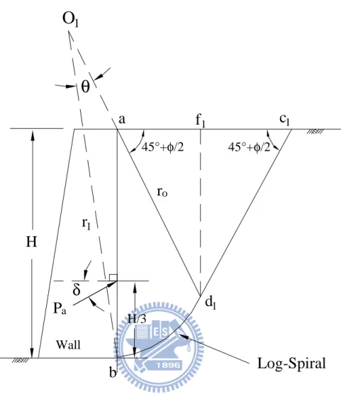
Fig. 2.5 illustrates the procedure to elevate the active resistance by trial wedge method (Terzaghi and Peck, 1967). The line d1c1 makes an angle of 45o +φ 2 with the surface of the backfill. The arc bd1 of trial wedge abd1c1 is a logarithmic spiral formulated as the following equation

r₁ =r₀eθtanφ (2.6)

O1 is the center of the log spiral curve in Fig. 2.5, where O1b = r1, O1d1 = r0, and ∠bO1d1 = θ. For the equilibrium and the stability of the soil mass abd1f1 in Fig. 2.6, the following forces per unit width of the wall are considered.

1. Soil weight per unit width in abd1f1: W1 = γ × (area of abd1f1)

2. The vertical face d1f1 is in the zone of Rankine’s active state; hence, the force

Pd1 acting on the face is

) 2 45 ( tan ) ( 2 1 2 2 1 1 φ γ °− = d d H P (2.7) where Hd1 = d1f1

(29)

upward from d1.

γ is the unit weight of soil

3. The resultant force of the shear and normal forces dF, acting along the surface of sliding bd1. At any point of the curve, according to the property of the logarithmic spiral, a radial line makes an angle φ with the normal. Since the resultant dF makes an angle φ with the normal to the spiral at its point of application, its line of application will coincide with a radial line and will pass through the point O1.

4. The active force per unit width of the wall P1 acts at a distance of H/3 measured vertically from the bottom of the wall. The direction of the force P1 is inclined at an angle δ with the normal drawn to the back face of the wall.

5. Moment equilibrium of W1, Pd1, dF and P1 about the point O1:

W₁

[ ]

l₂ +Pd₁

[ ]

l₃ +dF (0)= P₁

[ ]

l₁ (2.8) or

[

1 2 1 3

]

1 1 1 l P l W l P = + d (2.9)

where l2_{, l}3_{, and l}1_{are the moment arms for forces W}₁_{, P}_d1_{, and P}₁_{, respectively.}

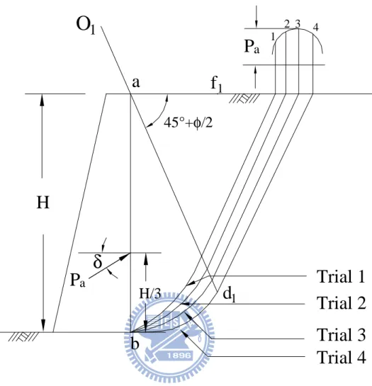
The trial active forces per unit width in various trial wedges are shown in Fig. 2.7. Let P1, P2, P3, …, and Pn be the forces that respectively correspond to the trial

wedges 1, 2, 3, …, and n. The forces are plotted to the same scale as shown in the upper part of the figure. A smooth curve is plotted through the points 1, 2, 3, …, n. The maximum P1 of the smooth curve defines the active force Pa per unit width of

(30)

2.1.4 Spangler and Handy’s Theory

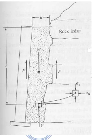
Spangler and Handy (1984) have applied Janssen’s (1895) theory to design problem of fascia retaining walls. Fig. 2.8 defines the soils with a width B bounded by two unyielding frictional boundaries (the rock face and wall face). The vertical force equilibrium of the thin horizontal soil element in Fig. 2.9 requires

dh V Bdh B V K dV V + )+2 µ = +γ ( (2.10)

This is a linear differential equation, the solution for which is

( ) µ γ µ K e B V B h K 2 1 2 / 2 − − = (2.11) where

µ = tan δ, the coefficient of friction between the soil and the wall

γ = unit weight of the soil

B = backfill width

h = backfill depth (i.e. z)

K = the coefficient of lateral earth pressure V = the vertical force

From the solution of eq.(2.11), an equation for lateral earth pressure σh can be

calculated = _ − − K ( )hB _ h e B µ µ γ σ 2 1 2 (2.12)

Some solutions for different values of B are shown in Fig. 2.10. The soil pressure, instead of continuing to increase with increasing values of h, levels off at a

(31)

δ γ µ γ σ tan 2 2 max B B h = = (2.13)

2.2 Laboratory Model Retaining Wall Tests

2.2.1 Model Study by Mackey and Kirk

Mackey and Kirk (1967) experimented on lateral earth pressure by using a steel model wall. This soil tank was made of steel with internal dimensions of 36 in.

× 16 in. × 15 in. (914 mm × 406 mm × 381 mm) as shown in Fig. 2.11. In this investigation, when the wall moves away from the soil, the earth pressure decreases (see Fig. 2.12) and then increases slightly until it reaches a constant value. Mackey and Kirk reported that if the backfill is loose, the active earth pressure obtained experimentally are within 14 percent off those obtained theoretically from almost any of the methods list in Table 2.1.

Mackey and Kirk utilized a powerful beam of light to observe the failure surface in the backfill. It could trace the position of the shadow, formed by changes of the sand surface in different level. It was found that the failure surface in the backfill due to the translational wall movement was approximated a curve in the backfill (Fig. 2.13), rather than a plane assumed by Coulomb.

2.2.2 Model Study by Fang and Ishibashi

Fang and Ishibashi (1986) conducted laboratory model experiments to investigate the distribution of the active stresses due to three different wall movement modes: (1) rotation about top, (2) rotation about base, and (3) translation. The experiments were conducted at the University of Washington.

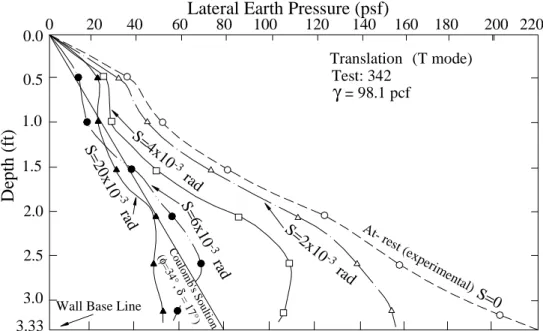
Fig. 2.14 shows the horizontal earth pressure distributions at different translational wall movements. The measured active stress is slightly higher than

(32)

Coulomb's solution at the upper one-third of wall height H is 3.33 ft (1.01 m), approximately in agreement with Coulomb's prediction in the middle one-third, and lower than Coulomb' at the lower one-third of wall surface. However, the magnitude of the active total thrust Pa at S = 20 10× −3 in. (0.5 mm) is nearly the same as that calculated from Coulomb's theory.

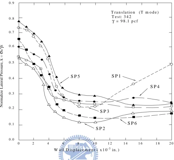
Fig. 2.15 shows lateral earth pressures measured at various depths decreased rapidly with the translational active wall displacement. Most measurements reach the minimum value at approximately 10 10× −3 in (0.25 mm, or 0.00025H) wall displacement and stay steady thereafter. Table 2.2 shows the range of wall displacement reported by previous researchers for the translational wall to achieve an active state.

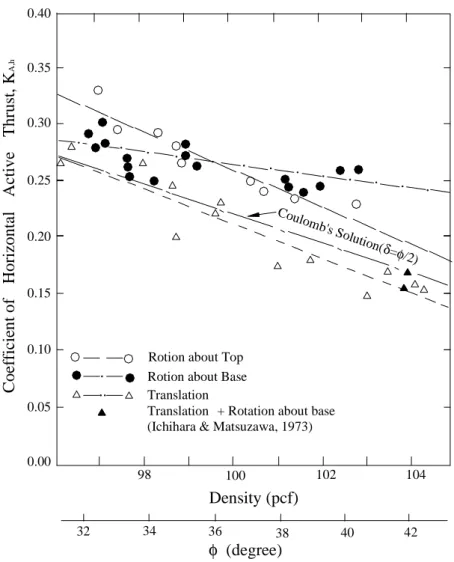
Fig. 2.16shows the Ka as a function of soil density and internal friction angle. In

this figure, the Ka value decreases with increasing φ angle. The Coulomb’s solution

might underestimate the coefficient Ka for rotational wall movements.

2.2.3 Model Retaining Wall Study by Huang

Huang (2009) used the model retaining wall facilities at National Chiao Tung University to investigate the active earth pressure on retaining walls near an inclined rock face. The backfill height H is 0.5 m. The parameters considered for that study were the rock face inclination angles β = 0°, 50°, 60°, 70°, 80°, 90°, the horizontal spacing b = 0, 50 mm, 100 mm as illustrated in Fig. 2.17 to Fig. 2.19.

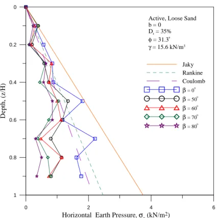
Fig. 2.20 to Fig. 2.22 shows the distribution of active earth pressure at different interface inclination angle for b = 0, 50 mm, 100 mm. Fig. 2.23 shows the active earth pressure coefficient Ka,h versus interface inclination angle β. The point of

application of active soil thrust versus interface inclination angle β is shown in Fig. 2.24. Based on the test result, the following conclusions are drawn:

1. With the approaching of the interface plate, the soil mass behind the wall decreased. The active earth pressure coefficient Ka,h decreased with

(33)

2. As the interface angle β increased or spacing b decreased (the rock face approached the wall face), the inclined rock face intruded the active soil wedge, the active pressure decreased near the base of the wall. This change of earth pressure distribution caused the active thrust to rise to a slightly higher location.

3. For all b = 0, b = 0.1H, and b = 0.2H, the horizontal component of active soil thrust Pa,h would decrease with increasing β angle. The intrusion of the inclined rock face would actually increase the FS against sliding of the wall. The evaluation of FS against sliding with Coulomb’s theory would be on the safe side.

2.2.4 Centrifuge Model Study by Frydman and Keissar

Frydman and Keissar (1987) used the centrifuge modeling technique to test a small model wall near a vertical rock face as shown in Fig. 2.25, and changes in pressure from the at-rest to the active condition was observed. The centrifuge system has a mean radius of 1.5 m, and can develop a maximum acceleration of 100 g, where g is the acceleration due to gravity. The models are built in an aluminum box of inside dimensions 327 × 210 × 100 mm. Each model includes a retaining wall made from aluminum (195 mm high × 100 mm wide × 20 mm thick) as shown in Fig. 2.26. The rock face is modeled by a wooden block, which can, through a screw arrangement, be positioned at varying distances b from the wall. Face of the block is coated with the sand used as fill, so that the friction between the rock and the fill is equal to the angle of internal friction of the fill. The granular fill between the wall and the rock face was modeled by uniform fine sand, the uniformity coefficient, Cu = 1.5. The model tests were carried out with the sand placed at a relative density of 70%. Simple shear tests performed on the sand at this relative density gave the angle of internal friction φ = 36°. Direct shear tests between the sand and aluminum yielded a friction angle 20°~25°.

(34)

Frydman and Keissar (1987) found that Spangler and Handy (1984) developed equation, (2.12) base on Janssen’s (1895) arching theory, for calculating the lateral pressure acting on the wall of a silo. In the silo, the lateral pressure σx at any given depth, z, is given as:

σx =             − − δ δ γ tan 2 exp 1 tan 2 b z K b (2.14) where

σx= lateral pressure acting on the wall (i.e. σh)

b = distance between silo walls

z = depth from top at which σx is required K = coefficient of lateral earth pressure γ = unit weight of the backfill

δ = angle of friction between the wall and the backfill

The coefficient K value depends on the lateral movement of the silo wall. For walls without any lateral movement, the Jaky’s equation was suggested for estimating the K value. In the active condition, Frydman and Keissar derived the K value by taking into account the friction between the wall and the fill, and assuming that the soil near the wall reached a state of failure. The K value is given by

(

) (

)(

)

(

4tan sin 1

)

1 sin tan 4 sin 1 1 sin ) 1 (sin 2 2 2 2 2 2 2 2 + − + − − − + − + = φ δ φ δ φ φ φ K (2.15)

Where φ = the angle of internal friction of the fill. The coefficient of lateral earth pressure in the active condition at given depth z can be determined as the ratio of

(35)

_            − − = δ δ 1 exp 2 tan tan 2 1 b z K z b K_a (2.16)

The coefficient of active earth pressures at given depth z for a retaining wall near a vertical rock face can be theoretically estimated by substituting Eq. 2.15 into Eq. 2.16. The distribution of Ka with the depth in Eq. 2.16 was verified using the experimental data obtained from the centrifuge model test, in which the wall rotated about its base (RB model). The Ka value obtained decreased considerably with depth. Additionally, the measured Ka value was significantly less than the Rankine’s or Coulomb’s coefficient of active earth pressure. Fig. 2.27 shows the distribution of Ka’ as a function of z/b. It is seen that for z/b less than about 1, the horizontal stress estimated using the silo pressure equation is greater than that corresponding to Rankine distribution. Obviously this is unacceptable. A more reasonable distribution may be obtained by assuming the silo pressure curve to be limited by the Rankine pressure, resulting in a composite curve such as ABC in Fig. 2.27.

2.3 Numerical Studies

2.3.1 Numerical Study by Leshchinsky, et al.

Leshchinsky, et al. (2004) used the limit equilibrium method with computer program ReSSA 2.0 (ADAMA, 2003) to numerically investigate the lateral earth pressure acting on a Mechanically-Stabilized-Earth wall. A baseline 5m-high wall was specified,the geometrical modeling was shown in Fig. 2.28(a). A single layer of reinforcement at 1/3 of the height of the wall was simulated in the analysis. In Fig. 2.28 the foundation was considered as competent bedrock to eliminate external effects on its stability. Various types of reinforced cohesionless fill were used in the analysis, all having a unit weight of γ = 20 kN/m3 and the internal angle of friction φ of the fill varying from 20° to 45°. Fig. 2.28(b) shows the base width of the fill was B, and the slope of the rear section of the fill was m.

(36)

Fig. 2.29 shows the results predicted by ReSSA versus values reported by Frydman and Keissar (1987). The bedrock constraining the sand in all tests was vertical (i.e., m = ∞). Frydman and Keissar (1987) reported an internal angle of friction of 36° and interface friction between the aluminum and sand δ = 20°~25°. Note that rather than using Ka’, the ratio Ka’/Ka is used, Ka = tan2(45°－φ/2) is Rankine’s active lateral earth pressure coefficient. Fig. 2.29 implies that as the retained soil space narrows (i.e., H/B increases) both ReSSA and the experimental data show the Ka’/Ka ratio decreases.

Fig. 2.30 presents the variation of active earth pressure coefficient Ka’ as a function of the rock face slope m. Ka’ was determined with the numerical analysis, and Ka was calculated with the Rankine theory Ka = tan2(45 ° －φ/2). The normalization of Ka’ with Ka produces charts that are independent of φ. For B = 0, the coefficient Ka’ rapidly decreased with increasing slope m. The amount of fill between the wall and bedrock was very small. For B = 0.1H and 0.2H, Ka’ also decreases with increasing slope m, however the space between the wall and the bedrock slope was becoming wider.

2.3.2 Numerical Study by Lawson and Yee

Lawson and Yee (2005) used the limit equilibrium method to numerically investigate the lateral earth pressure acting on retaining walls with constrained reinforced fill. The forces acting on the reinforced fill zone are shown in Fig. 2.31(a). The height of wall is H, and Lt is the width of fill at top. Lt/H represents the normalized with the height of fill. The destabilizing force is due to the weight of the fill, W, within the potential failure surface. For simplicity, it is assumed that the stabilizing force Ph acting on the rear of the wall face is horizontal and the wall face is vertical.

Fig. 2.31(b) shows values of earth pressure coefficient K for various wall Lt/H ratio for a fill with an internal friction angle φ’ = 30°. For L/H ratios greater than 0.5,

(37)

the active wedge can develop fully within the granular fill zone, hence the value of K = Ka = tan2(45°－φ/2) = 0.333. For Lt/H ratio less than 0.5, the active wedge cannot develop fully, hence the magnitude of K decreases for decreasing Lt/H.

2.3.3 Numerical Study by Yang and Liu

Yang and Liu (2007) used the finite element program Plaxis version 8 (Plaxis, 2005) to investigate the earth pressures for narrow retaining walls. Fig. 2.32 illustrates the narrow retaining walls in front of a stable rock face. L is the width of backfill and H is the height of wall. Fig. 2.33(a) shows the finite element mesh for at-rest condition, and Fig. 2.33(b) is the finite element model for active condition. The wall height H was fixed to 10 m while wall width L corresponding to desired wall aspect ratio L/H = 0.1, 0.3, 0.5, 0.7. Predicted earth pressure coefficients were normalized by Rankine Ka.

Normalized earth pressure coefficient profiles for at-rest condition are shown in Fig. 2.34(a), the earth pressure coefficient K0 decreases with decreasing aspect ratio L/H. Normalized earth pressure coefficient profiles for active condition are addressed in Fig. 2.34(b), the data are scattered around Ka and do not show a clear tendency. Even so, it can be observed that the earth pressure coefficient profiles decrease with decreasing aspect ratio. The effects of boundary constraint still can be recognized.

Fig. 2.35(a) shows the equivalent earth pressure coefficients Kw’ (along the wall face), Kc’(along the center of the backfill) and the equivalent earth pressure coefficients computed from arching equation for at-rest condition. All the pressure coefficients are normalized by Rankine Ka. The data from finite element analyses show the normalized equivalent earth pressure coefficients are less than K0/Ka by 10% to 60%, when the aspect ratio changed from 0.7 to 0.1.

Fig. 2.35(b) is the analytical results for active case. All pressure coefficients are normalized by Rankine Ka. The decreasing tendency of equivalent earth pressure from finite element analyses is not obvious until L/H < 0.3. This implies that the

(38)

boundary constraint starts to play a role when the shape of backfill become very slender. The difference between the earth pressures along the wall face and the earth pressures along the center of the backfill is apparent. This is most likely because all the stress points along the wall face are inside the failure wedge, but not all of stress points at the center of the backfill are at in the active wedge. Data from limit equilibrium analyses by Lawson and Yee (2005) and Leshchinsky et al. (2003) are compared with data calculated from finite element simulation. The results generally show a similar trend.

2.3.4 Numerical Study by Fan and Fang

Fan and Fang (2009) used the non-linear finite element program PLAXIS

(PLAXIS BV, 2002) to investigate the earth pressure against a rigid wall close to an inclined rock face (Fig. 2.36). The wall used for analysis is 5 m high, the back of the wall is vertical, and the surface of the backfill is horizontal. Typical geometry of the backfill zone used in the study is shown in Fig. 2.36. To investigate the influence of the adjacent rock face on the behavior of earth pressure, the inclination angle β of the rock face and the spacing b between the wall and the foot of the rock face were the parameters for numerical analysis. The wall was prevented from any movement during the placing of the fill. After the filling process, active wall movement was allowed until the earth pressure behind the wall reached the active condition. The finite element mesh, for a retaining wall with restrained backfill space (β = 70° and b = 0.5m) is shown in Fig. 2.37. The finite element mesh consists of 1,512 elements, 3,580 nodes, and 4,536 stress points.

Base on the numerical analysis, distributions of horizontal earth pressures with the depth (z/H) at various wall displacements for b = 0.5 m and β = 80° are shown in Fig. 2.38. In the figure, the distribution of active earth pressure with depth is non-linear. Due to the nearby rock face, the calculated active pressure is considerably less than

(39)

Fig. 2.39 shows the variation of the active earth pressure coefficient (Ka(Computed) / Ka(Coulomb)) as a function of the inclination angle β of the rock face and the wall-rock spacing b, for walls under translation movement. For β ＞ 60°, the analytical active K values are less than those calculated with Coulomb’s solution. The analytical K value decreased with increasing β angle.

Fig. 2.40 shows the variation of the location of active soil thrust with the β angle and wall-rock spacing b. For β ＞ 60°, the active soil thrust rises with increasing β angles, and the active h/H value increased with decreasing fill width b.

2.4 Plane Strain State-of-Stress

In many soil mechanics problems, a type of state-of-stress that is often

encountered is the plane strain condition. Referring to Fig. 2.41, for the retaining wall, the normal strain in the y direction at any point P in the soil mass is equal to zero (εy = 0). To reduce the side wall deflection, due to lateral earth pressure the NCTU model retaining wall (Fig. 1.7) used U-shaped steel beams and steel columns to confine the side walls deformation. The soil bin is nearly rigid that lateral deformation of side wall becomes negligible.

The normal stresses σy at all sections in the xz plane (intermediate principal plane) are the same, and the shear stresses on these xz planes are zero (τyx = τyz = 0). To minimun the side wall friction on xz plane, the NCTU model retaining wall uesd lubrication layers to reduce the interface friction between the sidewall and the backfill.

Under a plane-strain state of stress, the normal and shear stresses on the yz plane are equal to σx and τxz. Similarly, the normal and shear stress on the xy plane are σz and τzx (τzx = τxz). The relationship between the normal stresses can be expressed as

(40)

) ( ) ( E E E z x y y σ ν σ ν σ ε = − − (2.17)

where ν is Poisson’s ratio.

for a plane strain condition, εy = 0

z x y νσ νσ σ − − = 0

(

x z

)

y ν σ σ σ = + (2.18)

(41)

Chapter 3 Experimental Apparatus

In order to study the earth pressure behind retaining structures, the National Chiao Tung University (NCTU) has built a model retaining wall system which can simulate different kinds of wall movements. All of the investigations described in the thesis were conducted in this model wall, which will be carefully discussed in this chapter. The entire facility consists of four components namely, model retaining wall, soil bin, driving system, and data acquisition system. The arrangement of the NCTU model retaining wall system is shown in Fig. 3.1.

3.1 Model Retaining Wall

The movable model retaining wall and its driving systems are shown in Fig. 3.1. The model wall is a 1000-mm-wide, 550-mm-high, and 120-mm-thick solid plate, and is made of steel. Note that in Fig. 3.1 the effective wall height H is only 500 mm. The retaining wall is vertically supported by two unidirectional rollers , and is laterally supported by four driving rods. Two sets of wall-driving mechanisms, one for the upper rods and the other for the lower rods, provide various kinds of movements for the wall. A picture of the NCTU model wall facility is shown in Fig. 3.2.

Each wall driving system is powered by variable-speed motor. The motors turn the worm driving rods which cause the driving rods to move the wall back and forth. Fig. 3.3 shows two displacement transducers (Kyowa DT-20D) are installed at the back of retaining wall and their sensors are attached to the movable wall. Such an arrangement of displacement transducers would be effective in describing the wall

(42)

translation.

To investigate the distribution of earth pressure, nine earth pressure transducers were attached to the model wall. The arrangement of the earth pressure cells should be able to closely monitor the variation of the earth pressure of the wall with depth. Base on this reason, the earth pressure transducers SPT1 through SPT9 have been arranged at two vertical columns as shown in Fig. 3.4.

A total of nine earth pressure transducers have been arranged within a narrow central zone to avoid the friction that might exist near the side walls of the soil bin as shown in Fig. 3.5. The Kyowa model PGM-02KG (19.62 kN/m2 capacity) transducer shown in Fig. 3.6 was used for these experiments. To reduce the soil-arching effect, earth pressure transducers with a stiff sensing face are installed flush with the face of the wall. They provide closely spaced data points for determining the earth pressure distribution with depth.

3.2 Soil Bin

The soil bin is fabricated of steel members with inside dimensions of 2,000 mm

× 1,000 mm × 1,000 mm (see Fig. 3.1). Both sidewalls of the soil bin are made of 30-mm-thick transparent acrylic plates through which the behavior of backfill can be observed. Outside the acrylic plates, steel beams and columns are used to confine the side walls to ensure a plane strain condition.

The end wall that sits opposite to the model retaining wall is made of 100 mm thick steel plates. All corners, edges and screw-holes in the soil bin have been carefully sealed to prevent soil leakage. The bottom of the soil bin is covered with a layer of SAFETY-WALK to provide adequate friction between the soil and the base of the soil bin.

In order to constitute a plane strain condition, the soil bin is built very rigid so that the lateral deformations of the side walls will be negligible. The friction

(43)

that shear stress induced on the side walls will be negligible. To eliminate the friction between backfill and sidewall, a lubrication layer with 3 layers of plastic sheets was furnished for all model wall experiments. The “thick” plastic sheet was 0.152 mm thick, and it is commonly used for construction, landscaping, and concrete curing. The “thin” plastic sheet was 0.009 mm thick. It is widely used for protection during painting, and therefore it is sometimes called painter’s plastic. Both plastic sheets are readily available and neither is very expensive. The lubrication layer consists of one thick and two thin plastic sheets were hung vertically on each sidewall of the soil bin before the backfill was deposited (see Fig. 3.7). The thick sheet was placed next to the soil particles. It is expected that the thick sheet would help to smooth out the rough interface as a result of plastic-sheet penetration under normal stress. Two thin sheets were placed next to the steel sidewall to provide possible sliding planes. For more information regarding the reduction of boundary friction with the plastic-sheet method, the reader is referred to Fang et al. (2004).

3.3 Driving System

Fig. 3.1 shows the variable speed motors M1 and M2 (Electro, M4621AB) are employed to compel the upper and lower driving rods, respectively. The shaft rotation compels the worm gear linear actuators, while the actuator would push the model wall. To investigate the variation of earth pressure and the failure wedge caused by the translational wall movement, the motor speeds at M1 and M2 were kept the same speed of 0.015 mm/s for all experiments in this study.

3.4 Data Acquisition System

A data acquisition system was used to collect and store the considerable amount of data generated during the tests. The data acquisition system was composed of the

(44)

following four parts: (1) dynamic strain amplifiers (Kyowa: DPM601A and DPM711B); (2) NI adaptor card (NIBNC-2090); (3) AD/DA card; and (4) personal computers shown in Fig. 3.8. An analog-to-digital converter digitized the analog signals from the sensors. The digital data were then stored and processed by a personal computer. For more details regarding the NCTU retaining-wall facility, the reader is referred to Wu (1992) and Fang et al. (1994).

(45)

Chapter 4 Interface Plate and Supporting System

A steel interface plate is designed and constructed in the soil bin to simulate the constrained backfill shown in Fig. 1.1. In Fig. 4.1, the plate and its supporting system are developed to fit in the NCTU model retaining-wall facility. The interface plate consists of two parts: (1) steel plate; and (2) reinforcing steel beams. The supporting system consists of the following three parts: (1) top supporting beam; (2) base supporting block; and (3) base boards. Details of the interface plate and its supporting system are introduced in the following sections.

4.1 Interface Plate

4.1.1 Steel Plate

The steel plate shows in Fig. 4.2 is 1.370 m-long, 0.998 m-wide, and 5 mm-thick. The unit weight of the steel plate is 76.52 kN/m3 and its total mass is83 kg (814 N). A layer of anti-slip material (SAFETY-WALK, 3M) is attached on the steel plate to simulate the friction that acts between the backfill and rock face as illustrated in Fig. 4.2 and Fig. 4.3. For the wall height H = 0.5 m and the inclination angle β = 50o, the length of the interface plate should be at least 1.370 m. On the other hand, the inside width of the soil bin is 1.0 m. In order to put the interface plate into the soil bin, the width of the steel plate has to less than 1.0 m. As a result, the steel plate was designed to be 1.370 m-long and 0.998 m-wide.

4.1.2 Reinforcement with Steel Beams

To simulate the rock face shown in Fig. 1.1, the steel interface plate should be nearly rigid. To increase the rigidity of the 5 mm-thick steel plate, Fig. 4.2 (b) and Fig. 4.3 (b) shows 5 longitudinal and 5 transverse steel L-beams were welded to the back

(46)

of steel plate. Section of the steel L-beam (30 mm × 30 mm × 3 mm) was chosen as the reinforced material for the thin steel plate. On top of the interface plate, a 65 mm × 65 mm × 8 mm steel L-beam was welded to reinforce the connection between the plate and the hoist ring shown in Fig. 4.3 (b).

4.2 Supporting System

To keep the steel interface plate in the soil bin stable during testing, a new supporting system for the interface plate was designed and constructed. A top-view of the base supporting frame is illustrated in Fig. 4.4. The supporting system composed of the following three parts: (1) top supporting beam; (2) base supporting block and (3) base boards. These parts are discussed in following sections.

4.2.1 Top Supporting Beam

In Fig. 4.5, the top supporting steel beam is placed at the back of the interface plate and fixed at the bolt slot on the side wall of the soil bin. Details of top supporting beam are illustrated in Fig. 4.6. The section of supporting steel beam is 65 mm × 65 mm × 8 mm and its length is 1700 mm. Fig. 4.4 shows bolt slots were drilled on each side of the steel beam on the side wall of the soil bin. The locations of bolt slots were calculated for the interface plate at difference horizontal spacing b and inclined angle β. Fig. 4.7 shows the top supporting beam was fixed at the slots with bolts.

4.2.2 Base Supporting Block

The base supporting block used to support the steel interface plate is shown in Fig. 4.8. The base supporting block is 1.0 m-long, 0.6 m-wide, and 0.113 m-thick. Fig.4.8 shows seven trapezoidal grooves were carved to the face of the base

(47)

inserted into the groove at different distance from base of the model wall. In Fig.4.8, different horizontal spacing b adopted for testing includes: (1) b = 0; (2) b = 50 mm; (3) b = 100 mm; (4) b = 150 mm; (5) b = 250 mm; (6) b = 350 mm; and (7) b = 500 mm.

4.2.3 Base Boards

Fig. 4.5 shows 6 pieces of base boards are stacked between the base supporting block and the end wall, to keep the base block stable. The base boards show in Fig. 4.9 is 1400 mm-long, 1000 mm-wide and 113 mm-thick. To provide adequate friction between the backfill and the base board, the surface of the top base board was cover with a layer of anti-slip material SAFETY-WALK.

(48)

Chapter 5 Backfill and Interface Characteristics

This chapter introduces the properties of the backfill, and the interface characteristics between the backfill and the wall. Laboratory experiments have been conducted to investigate the following subjects: (1) backfill properties; (2) model wall friction; (3) side wall friction; (4) interface plate friction; and (5) distribution of soil density in the soil bin.

5.1 Backfill Properties

Air-dry Ottawa sand (ASTM C-778) was used throughout this investigation. Physical properties of the soil include Gs= 2.65, emax= 0.76, emin= 0.50, D60= 0.40

mm, and D10= 0.22 mm. Grain-size distribution of the backfill is shown in Fig. 5.1. Major factors considered in choosing Ottawa sand as the backfill material are summarized as follows.

1. Its round shape, which avoids effect of angularity of soil grains.

2. Its uniform distribution of grain size (coefficient of uniformity Cu=1.82), which avoids the effects due to soil gradation.

3. High rigidity of solid grains, which reduces possible disintegration of soil particles under loading.

4. Its high permeability, which allows fast drainage of pore water and therefore reduces water pressure behind the wall.

To establish the relationship between the unit weight γ of backfill and its

internal friction angle φ, direct shear tests have been conducted. The shear box used has a square (60 mm×60 mm) cross-section, and its arrangement is shown in Fig.

受限背填土對主動土壓力之影響

國立交通大學

國立交通大學

國立交通大學

國立交通大學

土木工程學系碩士班

土木工程學系碩士班

土木工程學系碩士班

土木工程學系碩士班

碩士論文

碩士論文

碩士論文

碩士論文

受限背填土

受限背填土

受限背填土

受限背填土對主動土壓力之影響

對主動土壓力之影響

對主動土壓力之影響

對主動土壓力之影響

Effects of Constrained Backfill on Active Earth Pressure

研

研

研

研 究

究

究

究 生

生

生

生 : 陳威廷

陳威廷

陳威廷

陳威廷

指導教授

指導教授

指導教授

指導教授 : 方永壽

方永壽

方永壽

方永壽 博士

博士

博士

博士

中

中

中

中 華

華

華

華 民

民

民

民 國

國

國

國 九十九

九十九 年

九十九

九十九

年

年 七

年

七

七 月

七

月

月

月

受限背填土

受限背填土

受限背填土

受限背填土對主動土壓力之影響

對主動土壓力之影響

對主動土壓力之影響

對主動土壓力之影響

Effects of Constrained Backfill on Active Earth

Pressure

研 究 生: 陳威廷

Student：Wei-Ting Chen

研究

究生

方永壽博士

中華

華民

民國

國九十九

九十九年

年七

七月

研究生: 陳威廷

指導教授：方永壽博士

國立交通大學土木工程學系碩士班

研究生 : 陳威廷指導教授 : 方永壽博士