國
立
交
通
大
學
電信工程研究所
碩 士 論 文
在 LTE 系統下保證服務品質的非連續接收機制週期調整方
法
A DRX Cycles Adjustment Scheme with QoS Guarantee in LTE System
研 究 生:施昌宏
指導教授:李程輝 教授
在 LTE 系統下保證服務品質的非連續接收機制週期調整
方法
A DRX Cycles Adjustment Scheme with QoS Guarantee in
LTE System
研究生:施昌宏 Student:Chung-Hung Shih
指導教授:李程輝 Advisor:Tsern-Huei Lee
國 立 交 通 大 學
電信工程研究所
碩 士 論 文
A ThesisSubmitted to Institute of Communications Engineering College of Electrical Engineering and Computer Engineering
National Chiao Tung University in partial Fulfillment of the Requirements
for the Degree of Master
in
Computer and Information Science
July 2012
Hsinchu, Taiwan, Republic of China
i
在 LTE 系統下保證服務品質的非連續接收機制週
期調整方法
學生: 施昌宏
指導教授:李程輝
國立交通大學電信工程研究所碩士班
摘
要
在長期演進計畫(LTE)系統中,為了節省用戶端設備 (UE) 的耗電,使待機時間延 長,系統使用了非連續接收機制 (DRX)。本論文中,我們將簡單介紹非連續接收 機制並進一步利用突發性封包模型 (bursty packet traffic model) 來表現此機制的 運作情形。對於不同流量的情況,我們藉由調整非連續傳輸機制週期 (DRX Cycles) 來加強節電效能。接著基於數學模型分析,探討非連續接收機制參數選取對於封 包延遲的影響。最後透過模擬結果顯示利用此方法確實可以降低能源消耗並滿足 封包延遲的要求以及如何在上述兩者之間權衡取捨。
ii
A DRX Cycles Adjustment with QoS
Guarantee in LTE System
Student:Chung-Hung Shih Advisor:Prof. Tsern-Huei Lee
Institute of Communications Engineering
National Chiao Tung University
ABSTRACT
In the Long Term Evolution (LTE) system, Discontinuous Reception (DRX) has been introduced for power saving to extend the battery life of the User Equipment (UE). In this thesis, we take an overview of the DRX mechanism and further analysis the mechanism with bursty packet traffic model. We propose a scheme for DRX Cycle adjustment to enhance the power saving performance in different traffic conditions. Based on the analytical model, effects of the DRX parameters on the packet delay performance are also investigated. Simulation results show that the scheme can reduce the power consumption with satisfying the packet delay requirement and a trade-off relationship between power saving and packet delay performance.
iii
目
錄
中文摘要
i
英文摘要
ii
目錄
iii
圖目錄
iv
表目錄
v
Chapter 1、 Introduction
1
Chapter 2、 Preliminary
3
2.1
Discontinuous Reception Mechanism
3
2.2
Packet Traffic Model
7
2.3
Related Work
8
Chapter 3、 Proposed Scheme for DRX Cycle Adjustment
10
3.1
System Model
10
3.2
Analytical Model
13
3.3
Comparison between Analytical and Simulation
Result
21
3.4
Selection Algorithm
26
Chapter 4、 Performance Evaluation
28
4.1
Parameters
28
4.2
Simulation Results
29
Chapter 5、 Conclusion
36
Bibliography
37
iv
圖 目 錄
Figure 1.1 UE’s traffic behavior
2
Figure 2.1 Frame structure
5
Figure 2.2 Simple illustration of DRX operation
6
Figure 2.3 Bursty packet traffic model [4]
7
Figure 3.1 System model
10
Figure 3.2 Packet delay by DRX
12
Figure 3.3 Illustration of delay by DRX
15
Figure 3.4 Regenerate cycle representation
16
Figure 3.5 Case 1: next burst arrives in mT
LC-E[N
k]T
SC16
Figure 3.6 Illustration of the next burst arrives in long cycle.
17
Figure 3.7 Case 2 : next burst arrives not in mT
LC18
Figure 3.8
Performance comparison among analytical results and
simulation results for different N
SC.
21
Figure 3.9
Performance comparison among analytical results and
simulation results for different T
SC.
23
Figure 3.10
Performance comparison among analytical results and
simulation results for different T
LC.
24
Figure 3.11 Flow chart of selection algorithm
26
Figure 4.1 The packet delay CDF of proposed scheme
30
Figure 4.2
Performance comparison among proposed scheme and
fixed cycle in delay bound 64ms
31
Figure 4.3
Performance comparison among proposed scheme and
fixed cycle in delay bound 128ms
32
Figure 4.4
Performance comparison among proposed scheme and
fixed cycle in delay bound 256ms
33
Figure 4.5
Performance comparison among proposed scheme and
v
表 目 錄
Table 2.1
Rule of On Duration Timer [1]
6
Table 2.2
Bursty packet traffic parameter distributions [6]
7
Table 3.1
DRX parameter values [12]
12
Table 3.2
Example
14
Table 3.3
Selection algorithm
27
Table 4.1
Parameters
29
Table 4.2
Parameters of Delay bound 64ms
32
Table 4.3
Parameters of Delay bound 128ms
32
vi
誌
謝
兩年碩士生涯隨著今年的畢業典禮結束也將告一段落,感謝李程輝
指導教授這兩年的諄諄引導。也感謝實驗室眾多熱心且經驗豐富的學
長姊:梓洋學長、承潔學姊、迺倫學姊、孟諭學長、啟全學長,分享
研究和生活的大小事,讓我碩班兩年的學習獲益良多。感謝這整個 NTL
大家族的各位:羅砲、嗣儒、玓仔、冠佑、家安、廣煜、咨翰、鱷魚、
阿肉、黑人;我的好室友們:小黃、志偉、香菇、許神、耕含、智偉、
景維,因為有你們,這兩年充滿了愉快的回憶!最後我想感謝我的家
人,感謝你們對我的包容和關懷,你們是我面對挑戰和困難時的慰藉
與動力。
1
Chapter 1.
Introduction
The 3rd generation partnership project (3GPP) is currently in the process of defining the long term evolution (LTE) as a mobile communication standard from the former 3G systems. UE energy saving is going to be an important issue of wireless network in recent years. Hence, in the released 3GPP specifications, LTE supports the power saving operation called Discontinuous Reception (DRX) mechanism to prolong the battery life of handset. The traffic status and DRX setting will directly influence the UE’s energy consumption.
UE can run many applications over time. Although user has no interaction with device, there exists background traffic due to open applications. In the view point of UE’s behavior, as seen in Figure 1.1, we characterize UE’s traffic by two states, i.e., active and background state. For background traffic, it doesn’t need high delay requirement. Therefore, we can set the DRX parameters to maximize the UE power saving. In active state, active traffic and background traffic coexist, but active traffic dominates this state. Based on different traffic types, active traffic may have various kinds of QoS requirements. For delay-sensitive traffic, we need to configure DRX parameters to meet the delay budget. Because of high traffic variability, using the same DRX parameters may not always be suitable. Switching parameters in each state and the impact of choosing different DRX parameters on packet delay should be considered.
2
Figure 1.1: UE’s traffic behavior
The outline of this article is organized as follows. Chapter 2 briefly introduces the DRX mechanism and the related works which we are going to adopt our system. System model, problem formulation and proposed algorithm are introduced in chapter 3. The following chapter 4 gives the performance evaluation. After that, a conclusion is drawn in chapter 5.
3
Chapter 2.
Preliminary
2.1
Discontinuous Reception Mechanism
A UE monitor a physical downlink control channel (PDCCH) in every subframe to determine whether resources are allocated in either downlink or uplink direction. The DRX mechanism is described in 3GPP LTE MAC specification [1]. It determines when the UE should monitor the PDCCH channel, or when should go to power saving mode. In the power saving mode, UE turns off its circuit to decrease the power consumption when there are no packet which needs to be transmitted or be received.
3GPP LTE specifies two radio resource control (RRC) states for UE, RRC_IDLE and RRC_CONNECTED states. DRX mode can be enabled in both RRC_IDLE and RRC_CONNECTED states. In the RRC_IDLE state, UE listens to the PDCCH, and receives the paging message from eNodeB about incoming call. Therefore, DRX mechanism in RRC_IDLE is used for non-consecutive listening to the call message in order to achieve the purpose of power saving.
In the RRC_CONNECTED state, when UE is initially establishing a radio resource link with eNodeB in the radio resource control link building process, the eNodeB will inform DRX mechanism parameters to UE. Besides, the initial values from RRC link setup, DRX parameters also can be updated via RRC connection reconfiguration
4
procedure. Therefore, in this state, UE power saving depends on the DRX parameter settings.
In this thesis, it focuses on DRX always in RRC_CONNECTED state (Full Connected DRX mode [2]). It means that UE will always stay in RRC_CONNECTED state with the proper DRX configuration. It has some advantages such as UE’s always-on service seems to have the guarantee and RRC signaling overhead on state transition is avoided completely. Respectively, the disadvantage is the increased power consumption. Therefore, we must use discontinuous reception mechanism in RRC_CONNECTED state to achieve the power saving.
The DRX mechanism contains several different parameters to control DRX operation [3]. These parameters are described in detail as follows and the DRX operation is illustrated in simplified form in Figure 2.1.
DRX Cycle: The DRX cycle specifies the periodic repetition of the On Duration followed by an inactive period. The mechanism provides two DRX Cycles that can be set for each UE, i.e. Long DRX Cycle (TLC) and Short
DRX Cycle (TSC). The former is necessary, and the latter is optional.
On Duration Timer (TON): The On Duration Timer specifies the number of
consecutive PDCCH subframe(s) at the beginning of a DRX Cycle. The UE will listens to the scheduling message on PDCCH during the period TON. If
the UE successfully decodes a scheduling message on PDCCH during the period TON, the UE will start or restart the Inactivity Timer.
5
Inactivity Timer (TIN): The Inactivity Timer specifies the number of
consecutive PDCCH subframe(s) after successfully decoding a PDCCH indicating an initial UL or DL user data transmission for this UE. Whenever a scheduling message is successfully received while the Inactivity Timer is running, the UE restarts the Inactivity Timer. If no scheduling message is received on PDCCH during the period TIN, the Inactivity Timer expired.
Short Cycle Timer (NSC): The Short Cycle Timer specifies the number of
consecutive subframe(s) the UE shall follow the Short DRX cycle. After the Short DRX Cycle is enabled, it will start or restart when the Inactivity Timer expired. When the Short Cycle Timer expires, the UE moves into a Long DRX Cycle.
In LTE standard, there are two-leveled unit of time: (1.) Frame (Radio frame) , and (2.) Subframe. Each frame is divided into ten subframes, and each frame has its own System Frame Number (SFN). Each subframe has their own subframe number from 1 to 10. These two units are used in DRX mechanism. Starting the On Duration Timer in every DRX Cycle has a rule which should be obeyed. This is shown in Table 2.1.
6
Table 2.1: Rule of On Duration Timer [1]
- If the Short DRX Cycle is used and [(SFN * 10) + subframe number] modulo (Short DRX Cycle) = (DRX Start Offset) modulo (Short DRX Cycle); or - if the Long DRX Cycle is used and [(SFN * 10) + subframe number] modulo
(Long DRX Cycle) = DRX Start Offset: - start On Duration Timer.
The DRX Start Offset is used to obtain the starting subframe number for DRX Cycle.
7
2.2
Packet Traffic Model
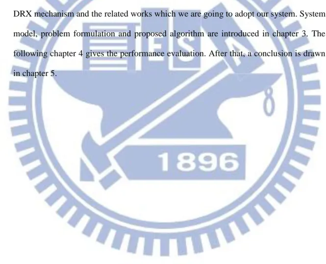
Figure 2.3: Bursty packet traffic model [4]
In this thesis, we measure the network traffic, and model it by a bursty packet traffic model [4], i.e. Figure 2.2. For this traffic model, an inter-packet arrival time and an inter-burst arrival time are generated by an exponential distribution. Each burst consists of several packets being generated by geometric distribution. The statistical distributions of the parameters in our traffic model are summarized in Table 2.2.
Table 2.2: Bursty packet traffic parameter distributions [6]
Parameter Distribution Mean Value
Inter-burst arrival time tib Exponential 1/λib
Number of packets per burst Np Geometric μp
8
2.3
Related Work
In DRX parameters configuration, the ideal situation to save the energy consumption is that a packet needs to be transmitted during UE’s on-duration and no packet needs to be sent in non-transmission period. Therefore, DRX mechanism should be compatible with traffic so that DRX mechanism can determine the parameters to achieve better energy saving.
In recent studies, the work [8][9][10] for DRX parameters impact have been proposed. The following is an overview of the study: The On Duration Timer and the Inactivity Timer are adopted to control UE’s power activity. When the length of the DRX cycle stays unchanged, the on-duration time (caused by On Duration Timer and Inactivity Timer) increasing makes UE power consumption increasing. In multi-user environment, considering the eNodeB resource scheduling, the On Duration Timer as well as the Inactivity Timer increasing will benefit the UE’s throughput. Using Short DRX Cycle, UE do not have to wait for the next regular Long DRX Cycle on-duration incoming.
[12] points out that the increasing of time to turn off the receiver will get a better power saving efficiency, but may increase the transmission delay between the UE and eNodeB. Hence, setting parameters in DRX configuration not only have to consider the packet interval, but also have to consider the quality of service requirements of each application.
The works in [5] have analyzed and modeled the UMTS power saving operation. Moreover, the performance of LTE DRX operation with bursty data traffic is discussed
9
in [6] and [7]. In these works, they analyzed that the power factor and the mean packet delay based on Poisson process, but they did not provide a selection algorithm for DRX configuration.
10
Chapter 3.
Proposed scheme for DRX Cycle
adjustment
Noted from chapter 2, the DRX parameters will significantly influence the performance of DRX operation under different traffic loads. In order to take appropriate adjustment, it is necessary to evaluate the performance over different parameter combinations in any traffic state. In this chapter, we are going to address the system model and the problem formation and then illustrate our analytical model and DRX parameter selection algorithm in detail.
3.1
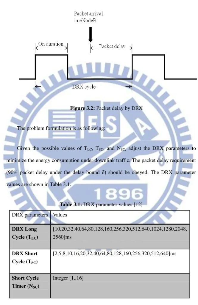
System Model
11
Our system model is shown in Figure 3.1. A Single eNodeB with a single UE is considered in this environment. Therefore, from the discussion in Section 2.3, we set the On Duration Timer and the Inactivity Timer enough value to operate DRX mechanism. It means when eNodeB has a packet in the buffer, it can successfully transmit the packet to UE during these enough value of time. In multi-user environment eNodeB should determine the scheduling of resource allocation. These two parameter values are based on the system load in the network. Now we just consider a single pair UE/eNodeB, so we choose the minimum value for On Duration Timer and the Inactivity Timer.
From Figure 1.1, we assume that we know the traffic characteristics in both two states. The background traffics generally have low data rate and large inter-arrival time, so we only use Long DRX Cycle with minimum Inactivity Timer and On Duration Timer to guarantee the packet delay bound in the background state. Then, we enable Short DRX Cycle to reduce the packet delay to meet the delay requirement in active state.
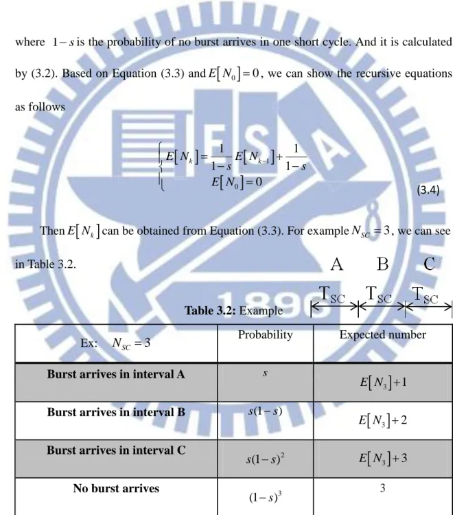
As seen in Figure 3.2, the packet delay is produced by using the DRX mechanism. If a packet arrives in eNodeB on UE’s off-duration of DRX Cycle, it will be stored in the buffer of eNodeB and will be transmitted to UE on the next on-duration of DRX Cycle. We define the time between packet arrival in eNodeB and the beginning of next on-duration DRX Cycle as packet delay.
12
Figure 3.2: Packet delay by DRX
The problem formulation is as following:
Given the possible values of TLC, TSC, and NSC, adjust the DRX parameters to
minimize the energy consumption under downlink traffic. The packet delay requirement (90% packet delay under the delay bound δ) should be obeyed. The DRX parameter values are shown in Table 3.1.
Table 3.1: DRX parameter values [12]
DRX parameters Values DRX Long Cycle (TLC) [10,20,32,40,64,80,128,160,256,320,512,640,1024,1280,2048, 2560]ms DRX Short Cycle (TSC) [2,5,8,10,16,20,32,40,64,80,128,160,256,320,512,640]ms Short Cycle Timer (NSC) Integer [1..16]
13
3.2
Analytical Model
Based on the traffic model of section 2.2, we assume that an inter-packet arrival time is shorter than an inter-burst arrival time. Therefore, if 1/
ib
p / ip, the burst packet traffic model can be simplified to Compound Poisson Process with parameter λib.And one burst contains μp packets on average.
We define t as inter-burst arriving time. Since the memoryless property of exponential distribution, it is true that
Pr( t XTSC| t )X Pr( t TSC)
For this reason, we can calculate two probabilities. The probability of no burst arrives in one short cycle is Pr( t TSC), and the probability of bursts arrive in one short cycle is Pr( t TSC). We summarize as follows,
Pr( > ) 1 Pr( ) 1 ib SC ib SC T SC T SC t T s e t T s e
Whenever a packet arrives in the serving eNodeB while UE is in the short cycle length and the Short Cycle Timer is running, the UE receives the packet in the next on-duration of short cycle and restarts the Short Cycle Timer. If no scheduling message is received on PDCCH during total short length, the Short Cycle Timer will expire and UE will move to long cycle. Therefore, the number of short cycle can be extended by the traffic. We defineN is the number of total short cycle whenk NSC k. And then, we
(3.1)
14
will derive it in next paragraph.
We can deriveE N
k by
k (1 )
k 1
1
k 1
1
k
E N s E N s E N E Nwhere 1 s is the probability of no burst arrives in one short cycle. And it is calculated by (3.2). Based on Equation (3.3) andE N
0 0, we can show the recursive equations as follows
1 0 1 1 1 1 0 k k E N E N s s E N ThenE N
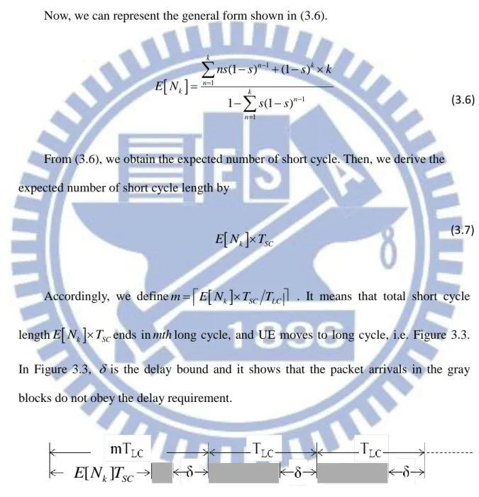
k can be obtained from Equation (3.3). For exampleNSC 3, we can see in Table 3.2.Table 3.2: Example
Ex: NSC 3 Probability Expected number
Burst arrives in interval A s
3 1E N
Burst arrives in interval B s(1s)
3 2E N
Burst arrives in interval C 2
(1 )
s s E N
3 3No burst arrives 3
(1s) 3
From the example, we summarizeE N by
3(3.3)
15
2
3 3 3 1 (1 ) 3 2 (1 ) 3 3 (1 ) 3 E N s E N s s E N s s E N s
3 2 2 3 2 (1 ) 3 (1 ) 3(1 ) 1 (1 ) (1 ) s s s p s s E N s s s s s Now, we can represent the general form shown in (3.6).
1 1 1 1 (1 ) (1 ) 1 (1 ) k n k n k k n n ns s s k E N s s
From (3.6), we obtain the expected number of short cycle. Then, we derive the expected number of short cycle lengthby
k SCE N T
Accordingly, we definemE N
k TSC TLC . It means that total short cyclelengthE N
k TSCends in mth long cycle, and UE moves to long cycle, i.e. Figure 3.3. In Figure 3.3, is the delay bound and it shows that the packet arrivals in the gray blocks do not obey the delay requirement.Figure 3.3: illustration of delay by DRX
(3.5)
(3.6)
(3.7)
[
k]
SC16
When a packet arrives in eNodeB on any UE’s Long DRX Cycle, it will be transmitted to UE during the next on-duration of long cycle. Then, UE starts the Short Cycle Timer once again. It forms a regenerate cycle as Figure 3.4.
Figure 3.4: Regenerate cycle representation
It can be divided into two conditions as shown in Figure 3.5 and 3.7 by whether the burst arrives in the gray block in Figure 3.5.
Figure 3.5: Case 1: next burst arrives in mTLCE N T[ k] SC
Case 1 is the condition of next burst arrives in the gray block, that is, in the period
[ ]
LC k SC
mT E N T . By DRX mechanism, the regenerate cycle will stop at the end of m-th TLC. The average number of bursts arrive in this case can be derived by
ib mTLC
17
where mTLC is the average regenerate cycle length of this case. Then, we derive the
average number of bursts arrive in the gray block of Figure 3.5 as shown by
ib mTLC E N Tk SC
Accordingly, in Figure 3.6 the probability of burst arrives in the gray block which means these bursts do not meet the delay requirement is derived by
( LC ) LC T T
Figure 3.6: illustration of the probability of burst arrives in the gray block
The probability of bursts arrives in the gray block in case 1 is smaller than (3.10).
Hence, the average number of bursts arrive in the gray block of Figure 3.5 and does not satisfy the delay requirement is shown in (3.11)
0 , 0 , 0 ib LC k SC LC k SC LC k SC LC k SC LC k SC mT E N T y mT E N T where y mT E N T mT E N T mT E N T Based on the properties of Poisson Process, we can calculate the probability of case 1 occur by
(3.11) (3.10)
18
- ( - [ ] ) 1-eib mTLCE N Tk SC
Now, we consider case 2 , no burst arrives in the gray block of Figure 3.4. As shown in Figure 3.6, it may cause the regenerate cycle extending until bursts arrival.
We define L asthe number of extended long cycles . Whenever a burst arrives in long cycle length, UE restarts short cycle. Based on memoryless property, the probability of bursts arrive in a long cycle length is 1e(ib LCT ). Thus, we can drive
E L by using the same method in (3.6).
( ) ( ) ( ) [ ] (1 ) 1 ( [ ] 1) 1 [ ] 1 ib LC ib LC ib LC T T LC LC T E L e e E L T E L T e
Figure 3.7: Case 2 : next burst arrives not in mTLC
The average length of case 2 is
m E L [ ]
TLCFrom (3.14), we derived the average number of bursts arrive in case 2 by adding the average number of bursts arrive in the gray block of case 2 with the average number of bursts arrive in mT . LC
(3.13) (3.12)
19
2 3
The average number of bursts arrive in the gray block of case 2
(1 ) (1 ) (1 ) 1 ib LC ib LC ib LC ib LC T T T ib LC ib LC ib LC ib LC ib LC T ib LC T e T e T e T T e E L T
Finally, we combine (3.8) and (3.15), then we have the average number of bursts arrive in case 2 in (3.16)
[ ]
ib m E L TLC
Thus, we can derive the average number of bursts which fails to meet delay requirement and arrive in the gray block of Figure 3.7 by
( ) ( ) 1 1 ib LC LC ib T LC LC T T e T
We calculate the probability of case 2 occur by
-ib(mTLC- [E N Tk]SC)
e
Due to (3.11), (3.12), (3.17), and (3.18), the average number of bursts fail to meet delay requirement in one regenerate cycle is less than
(3.15)
(3.17)
(3.18) (3.16)
20
- ( - [ ] ) ( [ ] ) [ ] 0 , 0 , 0 ib LC k SC LC ib LC k SC ib LC LC mT E N T LC k SC LC k SC LC k SC LC k SC T mT E N T y xE L T T where x e mT E N T y mT E N T mT E N T mT E N T By (3.9), (3.12), (3.14), and (3.18) we derive the average number of bursts arrive in one regenerate cycle by
- ( - [ ] ) - ( - [ ] )
(1- ib mTLC E N Tk SC ) ( ib mTLC E N Tk SC )( [ ])
ib e m e m E L TLC
Finally, we summarize the Equation (3.19) and (3.20). The probabilityPis shown in (3.21)
The average number of bursts fail to meet the delay bound requirement in one regenerate cycle The average number of bursts arrive in one regenerate cycle
( [ ] ) [ ] = LC ib LC k SC ib LC LC i P T mT E N T y xE L T T
- ( - [ ] ) (1- ) ( [ ]) 0 , [ ] 0 [ ] , [ ] 0 [ ] ib LC k SC b LC mT E N T LC k SC LC k SC LC k SC LC k SC x m x m E L T where x e mT E N T y mT E N T mT E N T mT E N T (3.21) (3.19) (3.20)21
3.3
Comparison between Analytical and Simulation Result
We have validated the analytical model against simulation experiments.
(a)
22
Figure 3.8: Performance comparison among analytical results and
simulation results for different NSC.
Figure 3.8 (a) shows the performance comparison among analytical results and simulation results, where TLC=256ms, TSC=64ms, δ=150ms, λ=0.001. Figure 3.8 (b)
shows the performance comparison among analytical results and simulation results, where TLC=256ms, TSC=128ms, δ=150ms, λ=0.001. We can see that when the number
of Short Cycle Timer increases, the probability of packet delay under the delay bound decreases. The reason is that using a bigger Short Cycle Timer tends to extend total Short Cycle Length. Therefore, UE takes more time in short cycles. It will reduce the probability of packet delay over the delay bound
23
(b)
Figure 3.9: Performance comparison among analytical results and simulation results for
different TSC.
Figure 3.9(a) is the performance comparison among analytical results and simulation results, where TLC=1024ms, NSC=8, δ=300ms, λ=0.001. Figure 3.9(b) is the
performance comparison among analytical results and simulation results, where TLC=512ms, NSC=12, δ=300ms, λ=0.001. It shows that the longer Short DRX Cycle is,
the lower probability of packet delay under the delay bound is. As mentioned above, it will reduce the probability of packet delay over the delay bound, too.
24
(a)
(b)
Figure 3.10: Performance comparison among analytical results and
simulation results for different TLC.
Figure 3.10(a) shows the performance comparison among analytical results and simulation results, where NSC=4, TSC=64ms, δ=75ms, λ=0.001. Figure 3.10(b) shows
25
NSC=6, TSC=64ms, δ=75ms, λ=0.005. As the Long DRX Cycle increases, the probability
of packet delay over the delay bound increases. Using longer Long DRX Cycle make the waiting time of packets increasing. Therefore, the number of packets which have to wait longer than the delay bound will rise.
From Figure3.8, Figure 3.9 and Figure3.10, we can find that the analytical results are slightly bigger than the simulation results. The reasons why the analytical results are bigger are that we use a bigger average number of packets fail to meet delay requirement and that we ignore the influence of On Duration Timer and Inactivity Timer in analytical model.
Note that the analytical results usually slightly smaller than the simulation results because the probability of case 2 occur we use is e-ib(mTLC- [E N Tk]SC) which is likely a
geometric mean. By the inequality of geometric and arithmetic mean, geometric mean is smaller than arithmetic mean. So, the analytical probability of case 2 occur is smaller than simulation results. However, the number of burst arrives in case 2 is bigger than the number of bursts arrives in case 1. Thus, the analytical average numbers of bursts arrive is smaller than simulation results. It will lead the probability of bursts fail to meet the delay requirement decrease.
The other reason is the calculation errors of average number of bursts fail to meet
the delay requirement in case 1. We use [ k] SC [ ]
ib LC k SC LC E N T T E N T T to
approach the actual average number [ k SC ]
ib LC k SC LC N T E T N T T .
26
3.4
Selection Algorithm
In this section, according to the analytical model derived in previous section, a selection policy for DRX Cycles is shown in Figure 3.11.
Figure 3.11: Flow chart of selection algorithm
27
After illustrating the ideas of our algorithm, the following table is pseudo codes of our algorithm.
Table 3.3: Selection algorithm
Algorithm : Proposed scheme for DRX Cycle adjustment SC : 1. 1024 16 2. ( ) 3. (1) SC ib d ON IN LC T SC d LC LC Inputs p T T default set T Max T N calculate P while P p
update T value to Next T end while while calculate P ( ) -1 ( ) 1 0 : d SC SC d SC SC d SC LC SC SC if P p update N N else if P p update N N end if break if P p or N end while Outputs T T N
28
Chapter 4.
Performance Evaluation
In this chapter, simulations are conducted to evaluate the performance of proposed scheme, which will be compared with the fixed DRX operation without adaptively adjusting DRX parameters.
4.1
Parameters
The probability of packet delay over the delay bound δ , p , is set to 0.9. And the d
delay bound δ is set to 64ms, 128ms, and 256ms. The parameters of the numerical simulation are listed in Table 4.1. A Single eNodeB and a single UE with downlink traffic is considered in this simulation environment. The On Duration Timer and Inactivity Timer are set as 2ms and 10ms for all cases. The value of Long Cycle based on the delay requirement in background state is assumed to be 1024ms, so we set the initial Long Cycle value as 1024ms.
29
Table 4.1: Parameters
4.2
Simulation Results
(a) Delay bound 64ms
ON IN
ip p
- =0.1
- The delay bound δ = 64, 128, 256ms - T =2ms, T =10ms
- Initial T 1024 - λ =1 arrivals/ms, μ =6
- Number of bursts in simulation = 10000 d
LC
p
ms
30
(b) Delay bound 128ms
(c) Delay bound 256ms
31
The packet delay CDF of proposed scheme is shown in Figure 4.4. In our scheme, we prove that the delay requirement (90% packet delay under the delay bound δ) in different inter-burst arrival time is obeyed. From the figure, we can see the packet delay CDF has linear-like relationship with delay. And the turning points of these lines occur in the delay valueTSC-T . ON
In the following figures, we show that the active ratio and delay probabilities respectively compare with fixed cycle scheme in different delay requirement as well as burst arrival rateib.Fixed cycle does not use Short Cycle in DRX operation, and use smaller fixed Long Cycle than delay bound instead.
(a) Active ratio (Delay bound 64ms) (b) Packet delay at 90% (Delay bound 64ms)
Figure 4.2: Performance comparison among proposed scheme and fixed cycle in delay
32
Table 4.2 Parameters of Delay bound 64ms (TSC 64ms)
(a) Active ratio (Delay bound 128ms) (b) Packet delay at 90% (Delay bound 128ms)
Figure 4.3: Performance comparison among proposed scheme and fixed cycle in delay
bound 128ms
Table 4.3 Parameters of Delay bound 128ms (TSC 128ms)
λib 0.0005 0.001 0.002 0.005 0.01 0.02 TLC 160 320 1024 1024 1024 1024 NSC 11 14 11 5 3 2 λib 0.0005 0.001 0.002 0.005 0.01 0.02 TLC 64 80 160 1024 1024 1024 NSC 0 11 14 11 7 4
33
(a) Active ratio (Delay bound 256ms) (b) Packet delay at 90% (Delay bound 256ms)
Figure 4.4: Performance comparison among proposed scheme and fixed cycle in delay
bound 256ms
Table 4.4 Parameters of Delay bound 256ms (TSC 256ms)
λib 0.0005 0.001 0.002 0.005 0.01 0.02
TLC 640 1024 1024 1024 1024 1024
34
(a) Active ratio (b) Packet delay at 90%
Figure 4.5: Performance comparison among proposed scheme and fixed cycle in
different delay bound
From Figure 4.5, it can be observed that the active ratio of proposed scheme is lower than the compared fixed cycle scheme but the packet delay is higher than the compared fixed cycle scheme. In other words, we sacrifice some packet delay to reduce the active ratio. From Table 4.2, Table 4.3, and Table 4.4, it is clear that instead of decreasing the Long DRX Cycle, enabling Short DRX Cycle with appropriate Short Cycle Timer can effectively decrease packet delay.
Then, we should note that as the value of ib increases, active ratio will increase
because the Inactivity Timer extends UE’s on-duration. When the value of delay bound is small, meeting the delay requirement will lead to increase in active ratio.
35
cycle scheme. That is because as the value of p increases, the time UE operates in d
short cycles also increases. When UE almost operates in short cycles, the performance will approach the fixed cycle scheme (the Short Cycle value used by our scheme is equal to the cycle value of fixed cycle scheme). The worst situation of our algorithm to select the DRX parameters with satisfying delay requirement is selecting the same as fixed cycle scheme. As seen in Table 4.2, in λib =0.0005 case we choose Long DRX
Cycle = 64ms and disable Short DRX Cycle to meet our delay requirement.
36
Chapter 5.
Conclusion
In this thesis, we take an overview of LTE DRX mechanism with adjustable DRX cycles and derive a mathematical model based on bursty packet traffic model. The analytical results match the simulation results. Through this model, we propose an algorithm for choosing DRX parameters. This algorithm tends to choose bigger long DRX cycle with smaller short cycle timer to satisfy the quality of service. Despite it may not have the guarantee to minimize the power consumption, it provides a simple way to choose DRX parameter with satisfying the delay requirement.
37
Bibliography
[1] 3GPP Technical Specification Group Radio Access Network, Evolved Universal Terrestrial Radio Access (E-UTRA) - Medium Access Control (MAC) protocol specification (Release 10), 3GPP TS 36.321 V10.5.0, Mar. 2012.
[2] CATT, “Signaling Overhead for IM traffic and Background traffic,” 3GPP TSG-RAN WG2 Meeting #77 R2-120258
[3] 3GPP Technical Specification Group Radio Access Network, Evolved Universal Terrestrial Radio Access (E-UTRA) and Evolved Universal Terrestrial Radio Access Network (E-UTRAN); Overall description; Stage 2(Release 11), 3GPP TS 36.300 V11.1.0, Mar. 2012.
[4] ETSI, “Universal Mobile Telecommunications System (UMTS); Selection Procedures for the Choice of Radio Transmission Technologies of the UMTS,” Technical Report UMTS 30.03, version 3.2.0, Apr. 1998.
[5] S. Yang, S. Yan, and H. Hung, “Modeling UMTS Power Saving with Bursty Packet Data Traffic,” IEEE Trans. Mobile Computing, vol. 6, no. 12, pp. 1398–1409, Dec. 2007.
[6] L. Zhou, H. Xu, H. Tian, Y. Gao, L. Du, and L. Chen, “Performance Analysis of Power Saving Mechanism with Adjustable DRX Cycles in 3GPP LTE,” Proc. IEEE VTC-fall, pp. 1–5, Sep. 2008.
[7] S. Jin, and D. Qiao, “Numerical Analysis of the Power Saving in 3GPP LTE Advanced Wireless Networks,” IEEE Trans. Vehicular Technology, vol. 61, no. 4, MAY. 2012.
38
[8] K. Aho, T. Henttonen, J. Puttonen and T. Ristaniemi, “Trade-off Between Increased Talk-time and LTE Performance,” International Conference on Networks (ICN) 2010.
[9] M. Polignano, D. Vinella, D. Laselva, J. Wigard, and T. B. Sorensens, “Power Savings and QoS Impact for VoIP Application with DRX/DTX Feature in LTE,” Proc. IEEE VTC-spring, pp. 1–5, May. 2011.
[10] J. Wigard, T. Kolding, L. Dalsgaard, C. Coletti, “On the User Performance of LTE UE Power Savings Schemes with Discontinuous Reception in LTE,” IEEE International Conference on Communications Workshops 2009.
[11] Research In Motion UK Limited, “DRX and Relationship to QoS,” 3GPP TSG-RAN WG2 Meeting #75bis R2-115246
[12] 3GPP Technical Specification Group Radio Access Network, Evolved Universal Terrestrial Radio Access (E-UTRA) - Radio Resource Control (RRC) protocol specification (Release 10), 3GPP TS 36.331 V10.5.0, Mar. 2012.
39
Appendix
Based on Section 3.1, we set the On Duration Timer and the Inactivity Timer minimum enough value to operate DRX mechanism. So we ignore the influence of On Duration Timer and Inactivity Timer in Section 3.2. In this chapter, we try to consider the influence of Inactivity Timer. When a burst arrives in the period of Inactivity Timer, it will restart another Inactivity Timer. If the longer T we use, the bigger impact of in Inactivity Timer it will be. Therefore, we must consider the impact of Inactivity Timer within big T . in
Now, we define R as the total time of T extended until in T expires. By using in
the same method in Equation (3.6) we have
1 1 1 1 (1 ) (1 ) [ ] 1 (1 ) in in in T T n in n T n n nq q q T E R q q
.where q is the probability of bursts arrive in one subframe. Then, we want to calculate a new [E Nk']to replace [E Nk], where E N[ k'] is the average number of total short DRX cycle length in one generating cycle with considering the Inactivity Timer. We define
W as the extended short DRX cycle after initial Inactivity Timer expired. As seen in
Table A.1, if a burst arrives in the interval A, B, or C, it will start the Inactivity Timer and reset the Short Cycle Timer.
40
Table A.1: Example
Ex: NSC 3 Probability Expected number
Burst arrives in interval A s
[ ] 1 SC E R E W T Burst arrives in interval B s(1s)
[ ]2 SC E R E W T
Burst arrives in interval C 2
(1 ) s s
3 [ ] SC E R E W T No burst arrives 3 (1s) 3 [ ] SC E R T From the example, we summarizeE W[ ]by
2 2 3 2 2 2 (1 ) 3 (1 ) 3(1 ) (1 ) (1 ) [ ] 1 (1 ) (1 ) 1 (1 ) (1 ) SC s s s s s s s s s s s E R E W s s s s s s s s s s T Thus, we have E N
3'
3 2 3 2 2 2 [ ] ' [ ] 2 (1 ) 3 (1 ) 3(1 ) (1 ) (1 ) [ ] [ ] 1 (1 ) (1 ) 1 (1 ) (1 ) SC SC SC E R E N E W T s s s s s s s s s s s E R E R s s s s s s s s s s T T Now, we can represent the general form
1 1 1 1 1 1 (1 ) (1 ) 1 [ ] ' 1 (1 ) 1 (1 ) k n k n k k k n n sc n n ns s s k E R E N T s s s s
41
Figure A.1: Performance comparison among analytical results and simulation results
for different TIN.
Figure A.1 shows the Performance comparison among analytical results and simulation results for different Tin where NSC=6, TSC=64ms, δ=75ms, λ=0.005
TLC=256ms. As we can see, the simulation results are similar to the analytical results.
Furthermore, the probability of bursts fail to meet the delay requirement will decrease with TIN increase.
Note that when Tin is small, they have similar probability of bursts fail to meet delay requirement. Thus, while using a small Tin, we can neglect the influence of Tin in analytical model.
![Table 2.1: Rule of On Duration Timer [1]](https://thumb-ap.123doks.com/thumbv2/9libinfo/8377820.178030/14.892.69.720.266.956/table-rule-duration-timer.webp)
![Figure 2.3: Bursty packet traffic model [4]](https://thumb-ap.123doks.com/thumbv2/9libinfo/8377820.178030/15.892.147.813.228.1057/figure-bursty-packet-traffic-model.webp)