應用Adjusted K-means方法選取適當的演化樹

國 立 交 通 大 學

統計學研究所

碩 士 論 文

應用Adjusted K-means方法選取適當的演化樹

Phylogenetic Tree Selection by the Adjusted K-means

Approach

研 究 生：洪珊琳

指導教授：王秀瑛 教授

應用Adjusted K-means方法選取適當的演化樹

Phylogenetic Tree Selection by the Adjusted K-means Approach

研 究 生：洪珊琳 Student：Shan-Lin Hung

指導教授：王秀瑛 博士

Advisor：Dr. Hsiuying Wang

國 立 交 通 大 學 理 學 院

統 計 學 研 究 所

碩 士 論 文

A Thesis

Submitted to Institute of Statistics College of Science National Chiao University

in Partial Fulfillment of the Requirements for the Degree of

Master in Statistics June 2009

Hsinchu, Taiwan, Republic of China

Phylogenetic Tree Selection by the Adjusted K-means

Approach

Student：Shan-Lin Hung Advisor：Hsiuying Wang

Institute of Statistics National Chiao Tung University

Hsinchu, Taiwan

Abstract

The reconstruction of phylogenetic trees is one of the most important and interesting problems of the evolutionary study. There are many methods proposed in the literature for constructing phylogenetic trees. Each method has its own criterion and bases on a selected evolutionary model. However, the topologies for the trees constructed from different methods may be quite different. The topology error may due to the unsuitable criterion or evolutionary model. Since there are many trees built from different methods, we are interested in selecting a valid tree. In this study, we propose an adjusted k-means approach and a misclassification error score criterion to solve the problem. This approach evaluates the trees by looking at the feature of the data from a statistical point view. It can provide an object criterion to select a valid tree from the statistics perspective. We apply the approach to the real data of phylogeny of the owlet-nightjars. It shows that the phylogeny tree constructed by Dumbacher et al. (2003) can reach minimum misclassification error score compared with the other several methods.

Keywords: Phylogeny tree, adjusted k-means, neighbor-joining method, minimum evolution

應用Adjusted K-means方法選取適當的演化樹

研究生：洪珊琳 指導教授：王秀瑛 博士

國立交通大學統計學研究所

摘要

演化樹的建立是演化研究裡重要又有趣的問題之一。在文獻中已經有許多有關演化 樹建的方法而每個方法都有自己的準則以及演化模型。然而，在建立演化樹過程中，這 些準則與演化模型有可能會導致演化樹在拓樸上的誤差。因為已經有許多不同的方法建 立演化樹，所以我們所感興趣的是選取可靠的演化樹。在這篇論文裡，我們提出adjusted

k-means方法與misclassification error score準則來解決問題。這個方法是利用統計的觀點

看資料的特質來評估演化樹。我們應用這個方法在Owlet-Nightjars的實際資料上，顯示

出Dumbacher et al.(2003)與其他方法所建構的演化樹，可以達到最小的misclassification

error score。

關鍵字： 演化樹，adjusted k-means，neighbor-joining 方法，minimum evolution 方法， maximum parsimony 方法，UPGMA 方法。

致謝

在交大統計所的兩年裡，「虛心學習、學以致用、團隊合作」是所上的老師以及同 學給了我在求學過程中前所未有的影響。在此，感謝所上的老師，謝謝老師細心的指引 我進入統計知識的殿堂，由於老師的諄諄教誨，使如同井底之蛙的我了解知識的浩瀚。 此外，感謝我所認識的同學以及朋友，因為他們陪伴與在學習上互相扶持，充實了我的 生活並且增貼許多色彩。而這篇論文的完成，完全要感謝王秀瑛教授的費心指導，因為 老師不斷的提供建議與方法，使我順利完成論文並且學習到如何學以致用。最後，最感 謝的就是我的家人，因為他們不斷的鼓勵、支持與陪伴，給了我無憂無慮的生活，讓我 擁有這一切。 洪珊琳 謹致于 國立交通大學統計學研究所 中華民國九十八年六月

0B

Contents

U ContentsU... 1 U 1.U UIntroductionU... 2 U 1.1U UMotivationU... 2 U 1.2U UTree-Building MethodsU... 2 U

1.3U UThe Models of Nucleotides SubstitutionU... 3

U

2.U UReal Data ExampleU... 4

U

2.1U UAvian FamilyU... 4

U

2.2U UFour Trees for Avian FamilyU... 5

U

3.U UAdjusted K-means Approach for Categorical DataU... 9

U

3.1U UClustering MethodU... 9

U

3.2U UThe Measure of DissimilarityU... 10

U

3.3U UAlgorithmU... 11

U

4.U UMisclassification Error ScoreU... 12

U

4.1U UMisclassification Error ScoreU... 12

U

4.2U UComparison of Misclassification Error ScoresU... 15

U

4.3U UThe Case of Excluding Aegotheles Savesi and Excluding the BothU... 17

U

5.U USimulation ResultU... 20

U

5.1U USimulation Based on Juke and Cantor ModelU... 20

U

5.2U USimulation ResultU... 20

U

1.

1B

Introduction

1.1

2B

Motivation

The reconstruction of phylogenetic trees is one of the most important and interesting problems of evolutionary study. There are many methods for constructing phylogenetic trees from molecular data: UPGMA (Sokal and Michener 1958), neighbor-joining (Saitou and Nei, 1987), minimum evolution (Rzhetsky and Nei 1992a, Saitou and Imanishi 1989, Kidd and Sgaramella-Zonta, 1971), maximum parsimony methods (Wiley 1981, Felsenstein 1982, Wiley rt al. 1991, Maddison and Maddison 1992, Swofford and Begle 1993) etc. When a phylogenetic tree is constructed, it is essential to know its accuracy. There are two types of errors in a phylogenetic tree: topological errors and branch length errors (Tateno et al. 1982). The former errors are differences in branching pattern between an inferred tree and the true tree, and the latter are deviations of estimated branch lengths from the true branch lengths. Topological errors are more serious than branch-length errors, and we mainly focus on topological errors in the study.

Since there are several methods for constructing phylogenetic trees, we focus on the comparison of different trees and propose a statistical approach to examine the accuracy of the topology of the trees. The computer simulation could be a good approach to explore the validity of the tree construction. However, for analyzing the multiple alignment DNA or protein sequences, the topologies for different trees constructed by different methods may be quite dissimilar. Although the bootstrap methods can be used to test the reliability of the tree, it still cannot be used to select the tree if the topology for each tree is dissimilar. In this study, we mainly consider the four kinds of tree constructed by UPGMA, neighbor-joining, minimum evolution and maximum parsimony methods, and propose a statistical method, the k-means cluster, to assist the selection of the correct tree. The building of four kinds of tree can be obtained after aligning the gene sequences by MEGA 4.1 software (Kumar et al. 2008, Tamura et al. 2007).

1.2

3B

Tree-Building Methods

There are many tree-building methods established in the literature. We focus on several methods in this study including UPGMA, minimum evolution (ME), neighbor joining (NJ)

and Maximum parsimony (MP) methods.

First, we introduce UPGMA (the Unweighted pair-group method using arithmetic averages), which is the simplest method in the category and there is a certain measure of evolutionary distance computed for all pairs of taxa or sequences in UPGMA, but the topological errors from UPGMA often occur when the rate of gene substitution is not constant or when the number of genes or nucleotides used is small.

For the minimum evolution (ME) method, it is computed for all or all plausible topologies, and the topology that has the smallest sum of all branch length estimates value is chosen as the best tree, however, a topology with the smallest sum of all branch length estimates value is not necessarily an “unbiased estimator” of the true topology.

The neighbor joining (NJ) method is based on the minimum evolution principle. This method doesn’t examine all possible topologies, but at each stage of taxon clustering a minimum evolution principle is used. The NJ method is regarded as a simplified version of the ME method. When four or five taxa are used, the NJ and ME methods give identical results (Saitou and Nei 1987).

Maximum parsimony (MP) method is originally developed for morphological characters (Henning 1966), and there are many different versions (Wiley 1981; Felsenstein 1982; Wiley et al. 1991; Maddison and Maddison 1992; Swofford and Begle 1993). Eck and Dayhoff (1966) seem to be the first to use an MP method for constructing trees from amino acid sequence data. Later, Fitch (1971) and Hartigan (1973) developed a more rigorous MP algorithm for nucleotide sequence data. In the MP method, the smallest number of nucleotide (or amino acid) substitutions that explain the entire evolutionary process for the topology is computed. This computation is done for all potentially correct topologies, and the topology that requires the smallest number of substitutions is chosen to be the best tree. However, MP methods tend to give incorrect topologies when there are backward and parallel substitutions at each nucleotide site and the number of nucleotides examined is rather small or when the rate of nucleotide substitution varies extensively with evolutionary lineage even if the number of nucleotides examined is very large (Felsenstein 1978).

1.3

4B

The Models of Nucleotides Substitution

As we mentioned in Section 1.1, the reconstruction of phylogenetic trees also based on the evolutionary models. In this section, the two common evolutionary models: Jukes and Cantor one-parameter model and Kimura two-parameter model, are introduced. The simulation study in Section 5 is based on the Jukes and Cantor one-parameter model.

Jukes and Cantor’s one-parameter model assumes that substitutions occur with equal probability, say  , among the four nucleotide types. Since the time of divergence between two sequences is usually unknown, we cannot estimate  directly. Instead, we compute K , the number of substitutions per site since the time of divergence between the two sequences. In the one-parameter model case, K 2 3

 

t , where 3 t is the expected number of

substitutions per site in a single lineage. Jukes and Cantor (1969) derived the following formula: 3 4 ˆ ln 1 4 3 K   _  p_   (1) where ˆp X L is the observed proportion of different nucleotides between the two sequences.

In the case of the two-parameter model (Kimura, 1980), the differences between two sequences are classified into transitions and transversions. Let Pˆ X₁ L and Qˆ X₂ L be the observed proportions of transitional and transversional differences between the two sequences, respectively, where X and 1 X2 are the numbers of transitional and

transversional differences between the two sequences. Then the number of nucleotide substitutions per site between the two sequences, K , is estimated by 2

2 1 1 1 1 ln ln ˆ ˆ ˆ 2 1 2 4 1 2 K P Q Q      _{ } _{ }        (2)

2.

5B

Real Data Example

2.1

6B

Avian Family

We use the avian family Aegothelidae discussed in Dumbacher, Pratt and Fleischer (2003) (commonly known as owlet-nightjars) to illustrate the aim of this study. Owlet-nightjars are small nocturnal birds related to the nightjars and frogmouths. Most are native to New Guinea, but some species extend to Australia, the Moluccas, and New Caledonia. There is a single monotypic family Aegothelidae with the genus Aegotheles. The family Aegothelidae comprises only 9 extant species, all in a single genus, Aegotheles.

Dumbacher, Pratt and Fleischer (2003) based on mitochondrial DNA sequence to construct a phylogeny of the owlet-nightjars. They analyzing mtDNA sequences Cytochrome b and ATPase subunit 8 suggests that 9 living species of owlet-nightjar and plus one that went

extinct early in the second millennium AD. They performed the maximum likelihood analyses, using the likelihood heuristic searches with a 2-rate class (transitions and transversions) model of sequence evolution with gamma correction, which is identical to the HKY85 model evolution (Hasegawa et al., 1985) with the addition of a gamma rate parameter (Yang, 1994). The taxon they used listed in Table 1 in Dumbacher et al. (2003) includes albertisi albertisi, wallacii wallacii, wallacii gigas etc. The Genbank numbers for the sequences are AY090664-AY090698 (for cytochrome b) and AY090699-AY090736 (for ATPase 8). A simple form of the tree based on the phylogeny results in Dumbacher, et al (2003) is referred to the website http://tolweb.org/tree/ of tree of life web project and is shown in Figure 1.

Figure1. A simple form of the tree for the avian family Aegothelidae constructed by Dumbacher, Pratt and Fleischer (2003).

Aegotheles archboldi (Archbold's Owlet-Nightjar) Aegotheles albertisi albertisi(Mountain Owlet-Nightjar) Aegotheles bennettii(Barred Owlet-Nightjar)

Aegotheles cristatus(Australian Owlet-Nightjar) Aegotheles tatei (Spangled Owlet-Nightjar) Aegotheles insignis (Feline Owlet-Nightjar) Aegotheles novaezealandiae *

Aegotheles savesi (Enigmatic Owlet-Nightjar) Aegotheles wallaciii (Wallace's Owlet-Nightjar)

Aegotheles albertisi salvadorii

Aegotheles crinifrons(Moluccan Owlet-Nightjar)

In Figure 1, branches that are represented by a hatched line rather than one solid bar indicate that the monophyly of the group may be uncertain. Aegotheles novaezealandiae in Figure 1 is the extinct one.

2.2

7B

Four Trees for Avian Family

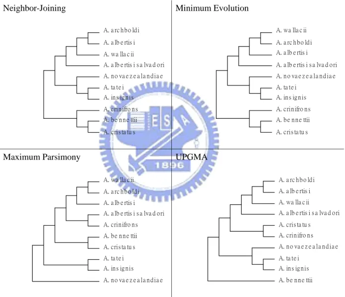
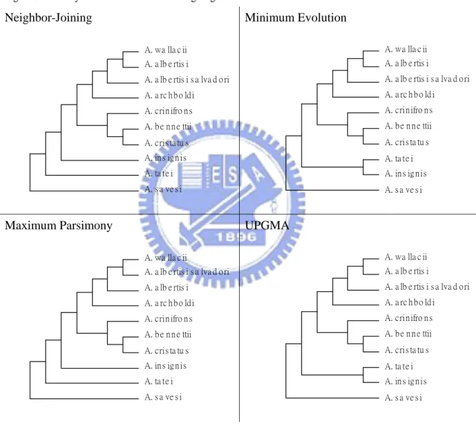
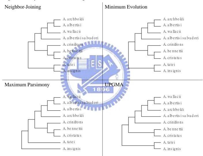
The four phylogenetic trees based on UPGMA, neighbor-joining, minimum evolution and maximum parsimony methods for cytochrome b plotted by MEGA software are shown in Figure 2, Figure 3, and Figure 4.

Figure 2. Trees by the four methods excluding Aegotheles savesi. Neighbor-Joining A. a rc h b o ld i A. a lb e rtis i A. ta te i A. in s ig n is A. b e n n e ttii A. cris ta tu s A. wa lla c ii A. a lb e rtis i s a lva d o ri A. n o va e z e a la n d ia e A. crin ifro n s Minimum Evolution A. wa lla c ii A. a rc h b o ld i A. ta te i A. in s ig n is A. b e n n e ttii A. cris ta tu s A. a lb e rtis i A. a lb e rtis i s a lva d o ri A. n o va e z e a la n d ia e A. crin ifro n s Maximum Parsimony A. wa lla c ii A. a rc h b o ld i A. a lb e rtis i s a lva d o ri A. crin ifro n s A. b e n n e ttii A. cris ta tu s A. ta te i A. in s ig n is A. a lb e rtis i A. n o va e z e a la n d ia e UPGMA A. a rc h b o ld i A. a lb e rtis i A. cris ta tu s A. crin ifro n s A. ta te i A. in s ig n is A. wa lla c ii A. a lb e rtis i s a lva d o ri A. n o va e z e a la n d ia e A. b e n n e ttii

Figure 3. Trees by the four methods excluding Aegotheles novaezealandiae. Neighbor-Joining A. wa lla c ii A. a lb e rtis i A. b e n n e ttii A. cris ta tu s A. a lb e rtis i s a lva d o ri A. a rc h b o ld i A. crin ifro n s A. in s ig n is A. ta te i A. s a ve s i Minimum Evolution A. wa lla c ii A. a lb e rtis i A. b e n n e ttii A. cris ta tu s A. a lb e rtis i s a lva d o ri A. a rc h b o ld i A. crin ifro n s A. ta te i A. in s ig n is A. s a ve s i Maximum Parsimony A. wa lla c ii A. a lb e rtis i s a lva d o ri A. b e n n e ttii A. cris ta tu s A. a lb e rtis i A. a rc h b o ld i A. crin ifro n s A. in s ig n is A. ta te i A. s a ve s i UPGMA A. wa lla c ii A. a lb e rtis i A. b e n n e ttii A. cris ta tu s A. a lb e rtis i s a lva d o ri A. a rc h b o ld i A. crin ifro n s A. ta te i A. in s ig n is A. s a ve s i

Figure 4.Trees by the four methods excluding the both. Neighbor-Joining A. a rc h b o ld i A. a lb e rtis i A. b e n n e ttii A. cris ta tu s A. wa lla c ii A. a lb e rtis i s a lva d o ri A. crin ifro n s A. ta te i A. in s ig n is Minimum Evolution A. a rc h b o ld i A. a lb e rtis i A. b e n n e ttii A. cris ta tu s A. wa lla c ii A. a lb e rtis i s a lva d o ri A. crin ifro n s A. ta te i A. in s ig n is Maximum Parsimony A. wa lla c ii A. a lb e rtis i s a lva d o ri A. b e n n e ttii A. cris ta tu s A. a lb e rtis i A. a rc h b o ld i A. crin ifro n s A. ta te i A. in s ig n is UPGMA A. wa lla c ii A. a lb e rtis i A. a rc h b o ld i A. a lb e rtis i s a lva d o ri A. crin ifro n s A. b e n n e ttii A. cris ta tu s A. ta te i A. in s ig n is

Form Figure 2, Figure 3, and Figure 4, the topologies built from the other four approaches are different from the tree proposed by Dumbacher et al. (2003). Without using a convincing criterion, it is not easy to compare their performances because each approach has its own merit. Thus, the aim of this study is to establish a reliable criterion from the statistics perspective to evaluate the different trees. A proposed method, the adjusted k-means approach, is introduced in the next section.

3.

8B

Adjusted K-means Approach for Categorical Data

3.1

9B

Clustering Method

A useful approach to classify the data is the clustering method (Anderberg, 1973; Jain and Dubes, 1988; Kaufman and Rousseeuw, 1990). The k-means clustering method proposed by MacQueen (1967) and Anderberg (1973) is a popular approach in the clustering methods to partition a set of objects into clusters such that objects in the same cluster are more similar to each other than objects in different clusters according to some defined criteria. However, the conventional k-means algorithm only works on numerical data, i.e., the variables are measured on a ratio scale (Jain and Dubes, 1988). This prohibits it from being used in applications where categorical data are involved. The nucleotide bases of a DNA sequence are A, T, C, G, which are categorical data as well as a protein sequence. The conventional k-means approach cannot be directly used to cluster the sequences.

Huang (1998) proposed an extension k-means algorithm, the k-modes algorithm, to categorical domains. We cannot directly apply conventional k-means approach to cluster the sequences, but we can adopt Huang’s approach to cluster the multiple nucleotide or protein sequences. However, the k-modes algorithm may not converge. Ng, Li, Huang and He (2007) provide a modified k-modes algorithm to overcome the converge problem of the original k-modes algorithm. Although the modified algorithm may be more stable than the original k-modes algorithm, according our computing results, it still cannot converge when it be applied to clustering the multiple nucleotide or protein sequences. Therefore, in this paper, we propose an adjusted k-means algorithm to cluster the multiple sequences. The algorithm is introduced in Procedure 1.

3.2

10B

The Measure of Dissimilarity

First we define the dissimilarity measure between the nucleotide or protein sequence X and a cluster nsequences n

G , where X 



x x_{1 2}x_m



is a nucleotide or protein sequence with length m, and Gn {G G₁n, ₂n,,G_nn} be a set of n nucleotide or protein sequences

with n



_{1 2}



i i i im

G  g g ...g . Note that

j

x represents the nucleotide in the j-th site of the sequence X and

ij

g represents the nucleotide in the j-th site of the i-th gene sequence,G_i, 1 i n, 1  , j m Then the dissimilarity measure between gene sequence X and cluster Gn is defined as the following





1 1 , ( , ) m n j i j j i n x g d X G n m    



, (3) where



xj,gi j

 

I gij xj



   and

 



I denotes the indicator function.

Assuming that _Gn1_,Gn2_,_,Gnk _{are k sets and each set has}

l

n sequences, l  , 1, ,k then we define the within group measure (WGM) and the between group measure (BGM) for



_Gn1_,Gn2_,_,Gnk



_{as follows:}





1 WGM for , \ for 1  



l   l l l l n n n n n i i i G d G G G l k (4),



1 2



1 2 1 2 2 1 1 2 1 2 1 1 BGM for , ( , ) ( , ) , and 1 ,   







   l l l l l l l l n n n n n n n n i i i i G G d G G d G G l l l l k (5),

where A\B denotes the set A excludes the element B.

Note that in the calculating of (3) after the alignment of the sequences, there may exist some missing sites for some sequences. For a specified site, it can be classified into three cases. The first one is that X is missing at this site. The second case is that all sequences in

n

G are missing at this site. And the third one is that some of the sequences in G are n missing at this site, but not all sequences. In the first or second case, the function 

 

 in (3)

is defined as 0. For the third case, we exclude the sequences with missing value at this site. Assume the number of the left sequences is r. Then we view the group G as a new set n G r with r sequences and calculate the dissimilarity measure under the assumption.

3.3

11B

Algorithm

Since our goal is to partition a set of objects into clusters such that objects in the same cluster are more similar to each other than objects in different clusters according to some defined criteria. Consequently, we prefer the between group measure is large and the within group measure is small. In this case, we set up a criterion to select the clusters such that

 *  *

M BGM WGM

is maximum, where *

BGM denotes all between group measures of each two clusters and

*

WGM denotes all within group measures described as equation (6) and equation (7), that is,



1 2







* 1 1 WGM for , , , , \ l k l l l n k n n n n n n i i l i G G G d G G G   



 (6),





1 1 2 1 2 1 2 1 * 1 1 BGM for , , , ( , ) l l l k n k k n n n n n i l l l i G G G d G G    

  

 (7).

Procedure 1.

Step1. Align the n sequences, X {X₁,X₂,...,X_n}, with MEGA.

Step2. Allocate every sequence to k clusters randomly.

Step3. Allocate a sequence to the cluster with the smallest dissimilarity measure according

to equation (3).

Step4. Repeat 3 until no sequence has changed cluster after a full cycle test of the whole

data set.

Step5. Repeat steps 2-4 m times and find the result in the m times with the largest M value, which are the required clusters.

The algorithm may not converge to the true clusters with maximum M value. Thus, Step 5 is provided to select the more accurate cluster.

4.

12B

Misclassification Error Score

4.1

13B

Misclassification Error Score

We use the avian family Aegothelidae to illustrate the adjusted k-means approach. In the approach, first the number of clusters, say k , needs to be determined. Since the goal of the 0

approach is to evaluate the performance of different tree methods, the selection of k is not 0

determined. We can evaluate the trees under the different cluster number and then conclude the best tree in which its performance is better in most situations. After applying the adjusted k-means approach in clustering the n sequences to k0 clusters, we define a

misclassification error score to evaluate a tree.

We take the tree constructed by Dumbacher et al. (2003) as an example to describe the misclassification error score calculation. Table 1 lists the cluster (excluding Aegotheles novaezealandiae) results by the approach for k0 2,...,9. For example, the third column in

Tables 1 is the cluster result of k 0 . The sequences (Aegotheles wallacii, Aegotheles 4

archboldi, Aegotheles albertisi, Aegotheles albertisi salvadori, and Aegotheles crinifrons) with respect to 1 are clustered to the first group; the sequences (Aegotheles tatei, and Aegotheles insignis) with respect to 2 are clustered to the second group and etc.

Table 1. The cluster results of the 10 sequences under different k0. 0 k 2 3 4 5 6 7 8 9 Aegotheles wallacii 1 3 1 1 1 6 8 6 Aegotheles archboldi 1 3 1 1 1 3 1 5 Aegotheles albertisi 1 3 1 1 1 3 1 5

Aegotheles albertisi salvadori 1 3 1 1 5 2 3 3

Aegotheles bennettii 1 1 4 4 6 4 7 4 Aegotheles cristatus 1 1 4 4 6 4 7 7 Aegotheles crinifrons 1 3 1 5 2 5 2 2 Aegotheles tatei 2 2 2 3 3 1 6 9 Aegotheles insignis 2 2 2 3 3 1 5 1 Aegotheles savesi 2 2 3 2 4 7 4 8

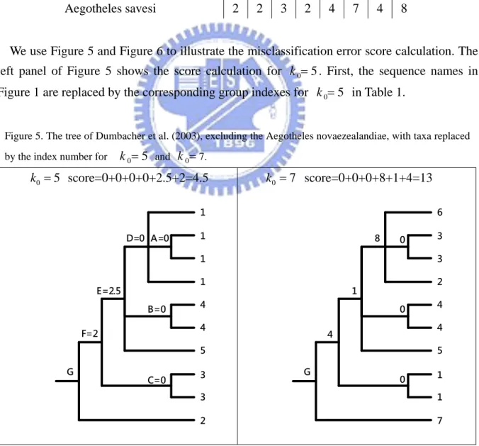
We use Figure 5 and Figure 6 to illustrate the misclassification error score calculation. The left panel of Figure 5 shows the score calculation for k₀5. First, the sequence names in Figure 1 are replaced by the corresponding group indexes for k₀5 in Table 1.

Figure 5. The tree of Dumbacher et al. (2003), excluding the Aegotheles novaezealandiae, with taxa replaced by the index number for k₀5 and k₀7.

0 5 k  score=0+0+0+0+2.5+2=4.5 1 1 4 4 3 3 1 1 B=0 5 E=2.5 C=0 F=2 D=0 A=0 2 G 0 7 k  score=0+0+0+8+1+4=13 3 3 4 4 1 1 6 2 0 5 1 0 4 8 0 7 G

Define the misclassification error score as the sum of the score at each node. The score at each node is the difference of the group index numbers of its branches. For example, in the right panel of Figure 5, there are 6 nodes, A, B, C, D, E, F that we need to count the score. Note that we do not count the score at the node G because all branches are spread out from this node. Thus, it is not necessary to require the small score at this node. The score value at each node is the absolute value of the difference of the branches spread from this node. Thus the misclassification error score is the sum of the five scores at these 5 nodes, which is calculated by 0+0+0+8+1=9.

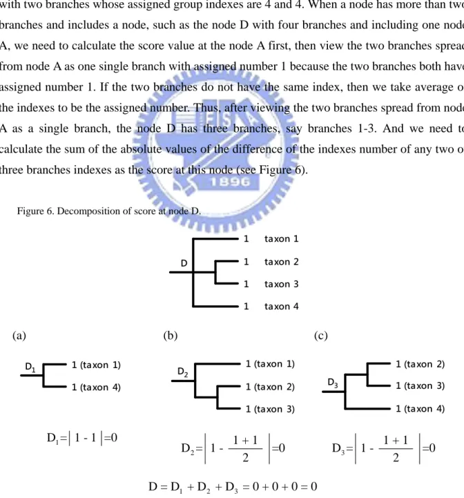
Note that for a node with only two branches, the score at this node is the absolute value of the difference of the two assigned group indexes, like the node B which has the score value 0 with two branches whose assigned group indexes are 4 and 4. When a node has more than two branches and includes a node, such as the node D with four branches and including one node A, we need to calculate the score value at the node A first, then view the two branches spread from node A as one single branch with assigned number 1 because the two branches both have assigned number 1. If the two branches do not have the same index, then we take average of the indexes to be the assigned number. Thus, after viewing the two branches spread from node A as a single branch, the node D has three branches, say branches 1-3. And we need to calculate the sum of the absolute values of the difference of the indexes number of any two of three branches indexes as the score at this node (see Figure 6).

Figure 6. Decomposition of score at node D.

1 taxon 2 1 taxon 3 1 taxon 1 1 taxon 4 D (a) 1 (taxon 1) 1 (taxon 4) D₁ (b) 1 (taxon 2) 1 (taxon 3) 1 (taxon 1) D₂ (c) 1 (taxon 2) 1 (taxon 3) 1 (taxon 4) D₃ 1 D = 1 - 1 =0 2 1 + 1 D = 1 - =0 2 3 1 + 1 D = 1 - =0 2 1 2 3 D = D + D + D = 0 + 0 + 0 = 0

Finally, when a node has included more than one node and a single branch without connecting a node such as node E, the score calculation is first calculating the average number of the branches of node D and node B, then take the absolute difference of the average number (1+1+4+4)/4 and the index 5 of the signal branch as the score at node E.

Here the average number (1+1+4+4)/4 is viewing the two branches at node B as a single branch and the two branches (taxon 1 and taxon 4) as a single branch. Here we do not need to consider the taxon 2 and taxon 3 here because its score has been considered at node A.

4.2

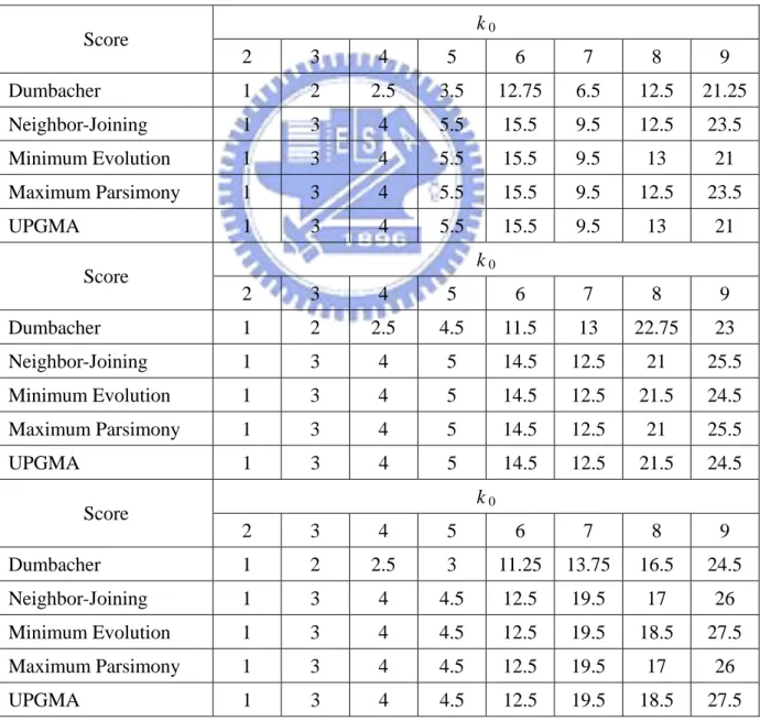
14B

Comparison of Misclassification Error Scores

With the definition of the misclassification error score, we can calculate the scores for the five trees constructed in Section 2 (Figure 3 and Figure 7) under different k . When 0 k = 2, 0

the five trees have the same misclassification error score. It cannot distinguish the performance of the five trees by the approach under the case. It due to that the rough classification with smaller cluster number which does not sufficiently use the information from the sequences cannot provide a useful aid in evaluating the performance of the tree construction methods. When we increase k , the results presented in Table 2 show that the 0

tree constructed by Dumbacher et al. (2003) has smallest misclassification error score among the trees for k =3, 4, 5, 6, 7, 8. 0

Note that for the case of k =9, the ME and UPGMA are shown to have smaller 0

misclassification error score than Dumbachers’ tree. Although the analysis for the case of

0

k = 9 is different from the cases of k =3, 4, 5, 6, 7, 8, we still can conclude that 0

Dumbachers’ tree has better performance compared with other threes for the avian family. Although the fact that we have different results for the cluster indexes at different time which may lead to different scores, it has little influence on the order of score for the trees. The scores in Table 2 are corresponding to different cluster number.

Figure 7. The tree constructed by Dumbacher et al. (2003) excluding A. novaezealandiae. A. archboldi A. albertisi albertisi A. bennettii A. cristatus A. tatei A. insignis A. wallaciii A. albertisi salvadorii A. crinifrons A. savesi

Table 2. The misclassification error scores for the five trees for k = 2, 3, 4, 5, 6, 7, 8 and 9 when the case exclude Aegotheles novaezealandiae

k 0 Score 2 3 4 5 6 7 8 9 Dumbacher 1 2 2.5 3.5 12.75 6.5 12.5 21.25 Neighbor-Joining 1 3 4 5.5 15.5 9.5 12.5 23.5 Minimum Evolution 1 3 4 5.5 15.5 9.5 13 21 Maximum Parsimony 1 3 4 5.5 15.5 9.5 12.5 23.5 UPGMA 1 3 4 5.5 15.5 9.5 13 21 k 0 Score 2 3 4 5 6 7 8 9 Dumbacher 1 2 2.5 4.5 11.5 13 22.75 23 Neighbor-Joining 1 3 4 5 14.5 12.5 21 25.5 Minimum Evolution 1 3 4 5 14.5 12.5 21.5 24.5 Maximum Parsimony 1 3 4 5 14.5 12.5 21 25.5 UPGMA 1 3 4 5 14.5 12.5 21.5 24.5 k 0 Score 2 3 4 5 6 7 8 9 Dumbacher 1 2 2.5 3 11.25 13.75 16.5 24.5 Neighbor-Joining 1 3 4 4.5 12.5 19.5 17 26 Minimum Evolution 1 3 4 4.5 12.5 19.5 18.5 27.5 Maximum Parsimony 1 3 4 4.5 12.5 19.5 17 26 UPGMA 1 3 4 4.5 12.5 19.5 18.5 27.5

4.3

15B

The Case of Excluding Aegotheles Savesi and Excluding the Both

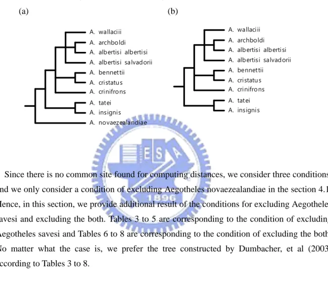
Figure 8. The tree constructed by Dumbacher et al. (2003) considered two conditions that excluding A. savesi (a) and excluding the both (b).

(a) A. archboldi A. albertisi albertisi A. bennettii A. cristatus A. tatei A. insignis A. wallaciii A. albertisi salvadorii A. crinifrons A. novaezealandiae (b) A. archboldi A. albertisi albertisi A. bennettii A. cristatus A. tatei A. insignis A. wallaciii A. albertisi salvadorii A. crinifrons

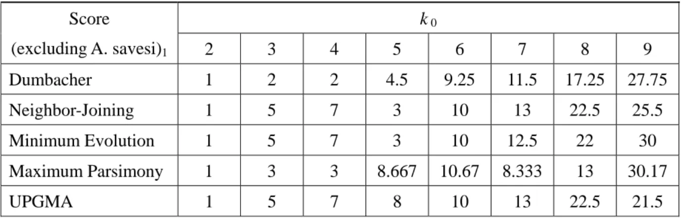
Since there is no common site found for computing distances, we consider three conditions, and we only consider a condition of excluding Aegotheles novaezealandiae in the section 4.1. Hence, in this section, we provide additional result of the conditions for excluding Aegotheles savesi and excluding the both. Tables 3 to 5 are corresponding to the condition of excluding Aegotheles savesi and Tables 6 to 8 are corresponding to the condition of excluding the both. No matter what the case is, we prefer the tree constructed by Dumbacher, et al (2003) according to Tables 3 to 8.

Table 3. k 0 Score (excluding A. savesi)1 2 3 4 5 6 7 8 9 Dumbacher 1 2 2 4.5 9.25 11.5 17.25 27.75 Neighbor-Joining 1 5 7 3 10 13 22.5 25.5 Minimum Evolution 1 5 7 3 10 12.5 22 30 Maximum Parsimony 1 3 3 8.667 10.67 8.333 13 30.17 UPGMA 1 5 7 8 10 13 22.5 21.5 Table 4. k 0 Score (excluding A. savesi)2 2 3 4 5 6 7 8 9 Dumbacher 1 2.5 2.5 1 7 14 18.25 25 Neighbor-Joining 1 3 3 5 11 10 21.5 24.5 Minimum Evolution 1 3 3 5 11 12 23 29 Maximum Parsimony 1 2 4 7.33 8.5 13 17.17 24.33 UPGMA 1 3 4 9 11 17 23.5 28 Table 5. k 0 Score (excluding A. savesi)3 2 3 4 5 6 7 8 9 Dumbacher 1 2 2.5 3.5 7.75 14.5 20.25 20.5 Neighbor-Joining 1 5 5 6 10 17 26 24 Minimum Evolution 1 5 5 6 10 16 24 26.5 Maximum Parsimony 1 3 2 7.5 6 15.17 16.33 22 UPGMA 1 5 5 6 10 17 26 22.5

Table 6.

k 0 Score

(excluding the both)1 2 3 4 5 6 7 8

Dumbacher 0 1 1.5 9 6.25 8.25 19.75 Neighbor-Joining 0 2 3 6 7 10 21 Minimum Evolution 0 2 3 6 7 10 21 Maximum Parsimony 1 3 4.5 10.5 9.5 9 19.5 UPGMA 0 2 3 6 8.5 11.5 25.5 Table 7. k 0 Score

(excluding the both)2 2 3 4 5 6 7 8

Dumbacher 0 1 1.5 5 8.25 13.25 10 Neighbor-Joining 0 2 3 5 11 12 13.5 Minimum Evolution 0 2 3 5 11 12 13.5 Maximum Parsimony 1 3 5 9.5 12 13 10.5 UPGMA 0 2 3 5 10 18 15 Table 8. k 0 Score

(excluding the both)3 2 3 4 5 6 7 8

Dumbacher 0 0.5 2.5 4.25 4.75 10.5 10

Neighbor-Joining 0 1 5 6 6 12 10.5

Minimum Evolution 0 1 5 6 6 12 10.5

Maximum Parsimony 1 2 5.5 7 8.5 7 11

5.

16B

Simulation Result

5.1

17B

Simulation Based on Juke and Cantor Model

Besides the owlet-nightjar example, we conduct a simulation study to investigate the feasibility of the k-mean approach.

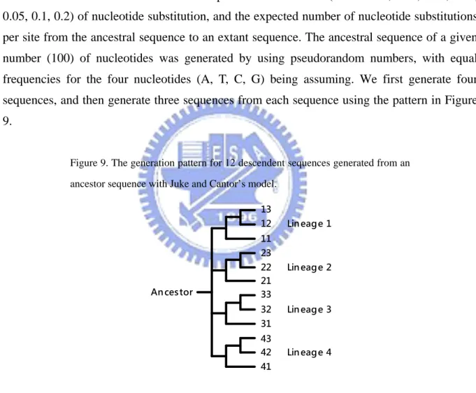
The trees were formed under the assumption of constant rate (rate = 0.01, 0.02, 0.03, 0.04, 0.05, 0.1, 0.2) of nucleotide substitution, and the expected number of nucleotide substitutions per site from the ancestral sequence to an extant sequence. The ancestral sequence of a given number (100) of nucleotides was generated by using pseudorandom numbers, with equal frequencies for the four nucleotides (A, T, C, G) being assuming. We first generate four sequences, and then generate three sequences from each sequence using the pattern in Figure 9.

Figure 9. The generation pattern for 12 descendent sequences generated from an ancestor sequence with Juke and Cantor’s model.

13 12 Lineage 1 23 22 Lineage 2 33 32 Lineage 3 43 42 Lineage 4 11 21 31 41 Ancestor

5.2

18B

Simulation Result

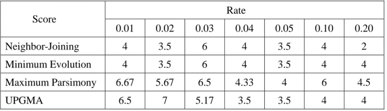
The misclassification error scores for the four trees under k0 4 for different substitution rate derived by the adjusted k-means approach are shown in Table 9.

Table 9. The misclassification error scores for four kinds of tree for different rates for 12 sequences generated from the model in Figure 9.

Rate Score 0.01 0.02 0.03 0.04 0.05 0.10 0.20 Neighbor-Joining 4 3.5 6 4 3.5 4 2 Minimum Evolution 4 3.5 6 4 3.5 4 4 Maximum Parsimony 6.67 5.67 6.5 4.33 4 6 4.5 UPGMA 6.5 7 5.17 3.5 3.5 4 4

We show the phylogeny trees for the rate 0.01 and 0.1 in Figures 10 and 11. Table 9 shows that in the case of rate being 0.01, the maximum parsimony and UPGMA trees has higher misclassification error score than the other two trees. From Figure 10, we can see that maximum parsimony and UPGMA trees have more dissimilar topologies from the topology of tree in Figure 9 than the other two trees. For the case of rate being 0.1, maximum parsimony tree has significantly higher misclassification error score than the other three trees. From Figure 11, the maximum parsimony tree has the most dissimilar topology from the tree in Figure 9 among the four trees.

From the simulation results, it shows that misclassification error score derived from the adjusted k-means approach can provide a convincing method to guide the selection of the valid tree.

Figure 10. The four trees for the 12 descendent sequences for rate 0.01 Neighbor-Joining 1 (3 1 ) 1 (3 3 ) 3 (1 2 ) 3 (1 3 ) 4 (4 1 ) 4 (4 2 ) 2 (2 2 ) 2 (2 3 ) 1 (3 2 ) 3 (1 1 ) 4 (4 3 ) 1 (2 1 ) Minimum Evolution 1 (3 1 ) 1 (3 3 ) 3 (1 2 ) 3 (1 3 ) 4 (4 1 ) 4 (4 2 ) 2 (2 2 ) 2 (2 3 ) 1 (3 2 ) 3 (1 1 ) 4 (4 3 ) 1 (2 1 ) Maximum Parsimony 3 (1 2 ) 3 (1 3 ) 3 (1 1 ) 1 (2 1 ) 2 (2 2 ) 2 (2 3 ) 1 (3 2 ) 1 (3 3 ) 1 (3 1 ) 4 (4 2 ) 4 (4 1 ) 4 (4 3 ) UPGMA 1 (3 1 ) 1 (3 2 ) 3 (1 2 ) 3 (1 3 ) 4 (4 1 ) 4 (4 3 ) 1 (3 3 ) 3 (1 1 ) 4 (4 2 ) 2 (2 2 ) 1 (2 1 ) 2 (2 3 )

Figure 11. The four trees for the 12 descendent sequences for rate 0.1 Neighbor-Joining 2 (2 2 ) 2 (2 3 ) 4 (3 2 ) 4 (3 3 ) 1 (1 2 ) 1 (1 3 ) 3 (4 2 ) 3 (4 3 ) 2 (2 1 ) 4 (3 1 ) 1 (1 1 ) 3 (4 1 ) Minimum Evolution 2 (2 2 ) 2 (2 3 ) 4 (3 2 ) 4 (3 3 ) 1 (1 2 ) 1 (1 3 ) 3 (4 2 ) 3 (4 3 ) 2 (2 1 ) 4 (3 1 ) 1 (1 1 ) 3 (4 1 ) Maximum Parsimony 2 (2 2 ) 2 (2 3 ) 4 (3 2 ) 4 (3 3 ) 1 (1 2 ) 1 (1 3 ) 2 (2 1 ) 4 (3 1 ) 1 (1 1 ) 3 (4 1 ) 3 (4 2 ) 3 (4 3 ) UPGMA 2 (2 1 ) 2 (2 2 ) 4 (3 2 ) 4 (3 3 ) 1 (1 2 ) 1 (1 3 ) 3 (4 1 ) 3 (4 3 ) 2 (2 3 ) 4 (3 1 ) 1 (1 1 ) 3 (4 2 )

19B

References

[1] Anderberg, M.R., 1973. Cluster for applications. Academic Press.

[2] Dumbacher, J. P., Pratt, T. K., and Fleischer, R. C., 2003. Phylogeny of the owlet-nightjars (Aves: Aegothelidae) based on mitochondrial DNA sequence. Molecular Phylogenetics and Evolution 29 (3): 540-549.

[3] Eck, R. V. and Dayhoff, M. O., 1966. Atlas of protein sequence and structure. National Biomedical Research Foundation, Silver Springs, MD.

[4] Felsenstein, J., 1978. Cases in which parsimony or compatibility methods will be positively misleading. Syst. Zool. 27:401-410.

[5] Felsenstein, J., 1982. Numerical methods for inferring evolutionary trees. Quart. Rev. Biol. 57: 379-404.

[6] Fitch, W. M., 1971. Toward defining the course of evolution: Minimum change for a specific tree topology. Syst. Zool. 20:406-416.

[7] Graur, D. and Li, W. H., 2000. Fundamentals of Molecular Evolution. Sunderland, Mass.: Sinauer Associates.

[8] Hartigan, J. A., 1973. HMinimum mutation fits to a given treeH. Biometrics 29:53-65.

[9] Hasegawa, M., Iida, Y., Yano, T. Takaiwa, F. and Iwabuchi, M., 1985a. Phylogenetic relationships among eukaryotic kingdoms inferred from ribosomal RNA sequences. J. Mol. Evol. 22: 32-38.

[10] Hasegawa, M., Kishino, H. and Yano, T., 1985b. Dating of the human-ape splitting by a molecular clock of mitochondrial DNA. J. Mol. Evol. 22: 160-174

[12] Huang, Z., 1998. Extensions to the k-means algorithm for clustering large data sets with categorical values. Data mining and knowledge discovery, Vol. 2, No. 3: 283-304.

[13] Jain, A.K. and Dubes, R.C., 1988. Algorithms for clustering data. Prentice Hall.

[14] Jukes, T. H., and Cantor, C. R., 1969.Evolution of protein molecules. In Mammalian protein metabolism (H. N. Munro, ed), pp. 21-132. Academic, New York.

[15] Kaufman, L. and Rousseeuw, P.J., 1990. Finding groups in data – An introduction to cluster analysis. Wiley.

[16] Kidd, K. K. and Sgaramella-Zonta, L. A., 1971. Phylogenetic analysis: Concepts and methods. Am. J. Hum. Genet. 23: 235-252.

[17] Kumar S, Dudley J, Nei, M and Tamura, K, 2008. MEGA: A biologist-centric software for evolutionary analysis of DNA and protein sequences. Briefings in Bioinformatics 9: 299-306.

[18] MacQueen, J., 1967. Some methods for classification and analysis of multivariate observations. Proc. Fifth Berkeley Symp. on Math. Statist. and Prob., Vol. 1 (Univ. of Calif. Press, 1967): 281-297.

[19] Maddison, W. P. and Maddison, D. R., 1992. MacClade: Analysis of phylogeny and character evolution. Sinauer Associates, Sunderland, MA.

[20] Ng, M. K., Li, M. J., Huang, J. Z. and He, Z., 2007. On the Impact of Dissimilarity Measure in k-Modes Clustering Algorithm. IEEE Transactions on HPattern Analysis and

Machine IntelligenceH, Vol. 29, No. 3: 503-507.

[21] Rzhetsky, A. and Nei, M., 1992a. A simple method for estimating and testing minimum-evolution trees. Mol. Biol. Evol. 9: 945-967.

[22] Saitou, N. and Imanishi, M., 1989. Relative efficiencies of the Fitch-Margoliash, maximum-parsimony, maximum-likelihood, minimum-evolution, and neighbor-joining methods of phylogenetic tree construction in obtaining the correct tree. Mol. Biol. Evol.

6: 514-525.

[23] Saitou, N. and Nei, M., 1987. The neighbor-joining method: A new method for reconstructing phylogenetic trees. Mol. Biol. Evol. 4: 406-425.

[24] Sokal, R. R. and Michener, C. D., 1958. A statistical method for evaluating systematic relationships. Univ. Kansas Sci. Bull. 28: 1409-1438.

[25] Swofford, D. L. and Begle, D. P., 1993. PAUP: Phylogenetic analysis using parsimony, ver. 3.1. user's manual. Illinois Natural History Survey, Champaign, IL.

[26] Tamura K, Dudley J, Nei, M and Kumar, S, 2007. MEGA4: Molecular Evolutionary Genetics Analysis (MEGA) software version 4.0. HMolecular Biology and EvolutionH 24:

1596-1599.

[27] Tateno, Y., Nei, M. and Tajima, F., 1982. Accuracy of estimated phylogenetic trees from molecular data. I. Distantly related species. J. Mol. Evol. 18: 387-404.

[28] Wang, H., Tzeng, Y.H. and Li, W.H., 2008. Improved variance estimators for one- and two-parameter models of nucleotide substitution. Journal of Theoretical Biology, 254: 164-167.

[29] Wiley, E. O., 1981. Phylogenetics: The theory and practice of phylogenetic systematics. Wiley, New York.

[30] Wiley, E. O., Brooks, D. R., Siegel-Causey, D. and Funk, V. A., 1991. The Compleat Cladist: A primer of phylogenetic procedures. Museum of Natural History, University of Kansas, Lawrence.

[31] Yang, Z., 1994a. Estimating the pattern of nucleotide substitution. J. Mol. Evol. 39: 105-111.

[32] Yang, Z., 1994b. Maximum likelihood phylogenetic estimation from DNA sequences with variable rates over sites: Approximate methods. J. Mol. Evol. 39: 306-314.

[33] Yang, Z., 1994c. Statistical properties of the maximum likelihood of phylogenetic estimation with distance matrix methods. Syst. Biol. 43: 329-342.