應用於合作無線隨意網路中利用增加空間性頻道使用來增進效能之中繼點選擇機制

(1)

國

立

交

通

大

學

網路工程研究所

碩

士

論

文

應用於合作無線隨意網路中利用增加空間

性頻道使用來增進效能之中繼點選擇機制

A Relay Selection Scheme with Enhancing Spatial

Channel Reuse in Cooperative Wireless Ad Hoc Networks

研究生：張景翔

指導教授：趙禧綠助理教授

(2)

摘要

在近幾年內，學者們提出了一類稱為合作通訊的方法，這類方法能使配備單一天線的行動裝置在多使用者的環境中分享彼此的天線以建立一個虛擬化的多天線傳送端。由於花費或是硬體上的限制，行動裝置可能沒辦法配備多天線。但透過合作通訊，一個配備單一天線的行動裝置也能在多使用者的環境中以虛擬化的多天線傳送端達到發射分送的效果。在這篇論文中，我們提出了一種中繼點選擇機制，針對中繼點附近傳輸的多寡等情形挑選出一個被影響較少也影響其他傳輸較少的中繼點，而這個方法是為了要達到空間性頻道重複使用最大化的目的。透過使用 ns-2 網路模擬器，我們評估了使用這個方法的效能。實驗結果顯示，即使是受到鄰近傳輸的影響，較為穩定增加的網路吞吐量以及所維持之降低的網路延遲時間表現出了使用這個方法的優越之處。

(3)

Abstract

In the last few years, a new class of methods called cooperative communication has been proposed that enables single-antenna mobiles in a multi-user environment to share their antennas and generate a virtual multiple-antenna transmitter. A mobile station may not be able to support multiple transmit antennas due to some hardware limitations. Through cooperative communication, a single-antenna mobiles in a multi-user environment can utilize the virtual multiple-antenna transmitter to achieve the transmit diversity. In this thesis, we propose a relay selection scheme which considers neighbor traffic of the relay node in order to maximize the spatial channel reuse in the cooperative communication. Through the simulation with ns-2 simulator, we evaluated the performance of the proposed scheme. As presented by the simulation results, the more stable increase in the total network throughput and the reduction in delay even when affected by neighbor traffics show the outperformance by utilizing the proposed scheme.

(4)

致謝

終於，能完成這份論文，也算是為兩年研究生涯劃下一個句點。想當初，在步入實驗室的那天，雖知道要走到今天這一步肯定要花不少功夫。但在經歷過這一段時光後，才知道做研究可真是不簡單。在這段研究期間裡，曾遭遇種種的挫折，從閱讀、搜索及整理相關研究資料到發現問題與思考解決方法，甚至為方法或演算法寫模擬跑實驗，所會出現的問題是當初天真的我所未能料想得到的。但在遇上問題的時候，總是有許多貴人相助，在此，我要感謝這些幫助我的人。首先，我要感謝我的指導教授 - 趙禧綠老師。在這兩年研究的日子裡，儘管自己多次地犯錯或表現未佳，老師仍不厭其煩地指導與給予鼓勵，一步一步地指引方向引領前進。雖然多次的挫折令我幾乎想懦弱地逃避，老師卻未曾放棄我，這也才能讓我走到今天這一步。接著，我要感謝實驗室的大家。在平日的相處之中，相互的精神砥礪與打氣使我能每天都有勇氣接受挑戰與被挫折後再爬起的動力。感謝學長姊的照顧與不吝指教、同學的激勵鼓舞和相助以及學弟妹的幫忙與對不才的忍受。有了你們，才能使苦悶的研究生活更添一份色彩。最後，要感謝我的父母家人及朋友，讓我總是在我最無助的時候還能找到永遠支持我的人，聽我訴苦及給予安慰與幫助。沒有在背後默默支持的你們，我也沒有完成論文的這天。感謝所有曾幫助過我的人，謝謝你們。

(5)

List of Figures

Figure 1-1 The concept of cooperative communication... 2

Figure 1-2 The extended sensing area... 3

Figure 2-1 Basic CMAC protocol ... 6

Figure 2-2 Cooperative regions for CoopMAC... 7

Figure 2-3 Control frame and Data frame exchange in CoopMAC ... 8

Figure 2-4 The “best” relay among M candidates is selected to relay information ... 8

Figure 2-5 Control frame and Data frame exchange in opportunistic relaying ... 9

Figure 3-1 Data structure of a neighbor table... 12

Figure 3-2 Illustration of information gathering ... 14

Figure 3-3 802.11 MAC with Direct transmission... 16

Figure 3-4 Cooperative MAC with two hop transmission ... 17

Figure 3-5 Cooperative MAC with Direct transmission... 19

Figure 3-6 The scenario for the example which illustrates the algorithm. ... 20

Figure 3-7 An illustration of the scheme to improve the spatial channel reuse... 21

Figure 4-1 Topology of Scenario 1... 26

Figure 4-2 Service Delay of 802.11 vs. OR vs. NAV-RS with different hello message intervals ... 27

Figure 4-3 Throughput of 802.11 vs. OR vs. NAV-RS in different hello message intervals... 27

Figure 4-4 Service Delay of 802.11 vs. OR vs. NAV-RS in Scenario 1 ... 28

Figure 4-5 Throughput of 802.11 vs. OR vs. NAV-RS in Scenario 1... 29

Figure 4-6 Flow 0-1’s throughput of 802.11 vs. OR vs. NAV-RS in Scenario 1 ... 30

Figure 4-7 Transmission times of 802.11 vs. OR vs. NAV-RS in Scenario 1... 30

Figure 4-8 Loss rate of 802.11 vs. OR vs. NAV-RS... 31

Figure 4-9 Transmission cost of 802.11 vs. OR vs. NAV-RS ... 32

Figure 4-11 Service Delay of 802.11 vs. OR vs. NAV-RS in Scenario 2 ... 34

Figure 4-12 Throughput of 802.11 vs. OR vs. NAV-RS in Scenario 2... 35

Figure 4-13 Flow 0-1’s throughput of 802.11 vs. OR vs. NAV-RS in Scenario 2 ... 35

Figure 4-14 Transmission times of 802.11 vs. OR vs. NAV-RS in Scenario 2... 36

Figure 4-15 Loss rate of 802.11 vs. OR vs. NAV-RS in Scenario 2... 37

Figure 4-16 Transmission costs of 802.11 vs. OR vs. NAV-RS in Scenario 2 ... 37

Figure 4-18 Throughput of 802.11 vs. OR vs. NAV-RS with different packet size ... 38

Figure 4-19 Throughput gain of OR vs. NAV-RS... 39

(7)

List of Tables

Table 2-1 Comparison of relay selection schemes in different protocols... 11 Table 4-1.Intersil HFA3861: The Relationship between BER and SNR & Modulation...24 Table 4-2.Parameters used in this simulation ... 24

(8)

Chapter1 Introduction

1.1 An Overview of Cooperative Communication

In recent years, since wireless local area networks have arrived to provide an alternative to LANs which is based on cable and optical fiber, it brings us lots of benefits that eliminates the wiring cost and accommodates mobile stations. With the low cost and mobility, the WLANs become more and more popular.

Wireless is convenient and less expensive to deploy, but it is not perfect. There are many limitations to prevent wireless technologies from reaching their full potential. One of the limitations is the transmission medium. The strength of a signal falls off with distance over any transmission medium, but it is worse for the wireless because of free space loss, noise, and fading caused by changes in the transmission medium or path(s). Mobility is an advantage of wireless, but it also causes the effect of fading.

In wireless environment, the communication quality often degrades due to distance and fading. The communication state determines the performance of transmission. When the communication state gets worse, the received signal may be in error. Once the error bits in a transmitted packet are too much to be decoded correctly, this packet will be dropped even be loss if it is dropped again and again until exceeding the retransmission threshold.

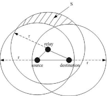
If the communication quality between the transmitter and receiver is too bad to remain the low loss rate, the packets may start to be dropped and pending for retransmission. Because of the broadcast nature of the wireless medium, neighbor nodes can overhear the transmission from the sender in the wireless channel environment. Through the broadcast nature of the wireless medium, the packets overheard by relay nodes can be stored and forward to the destination instead of being retransmitted by the source. This is the basic idea of the cooperative communication, as the Fig. 1-1.

(9)

Figure 1-1 The concept of cooperative communication

The concept of cooperation was introduced in [1]. Cooperative communication schemes are classified into three types: store and forward [2, 3], amplify and forward [4] and coded cooperation [5, 6]. Type 1, store and forward - the partner receives the transmitter’s data and retransmits the data to the destination. Type 2, amplify and forward - each partner receives the signal by the source then amplifies and retransmits it and the receiver combines the signal transmitted by the source and partner to obtain the final signal. Type 3, coded cooperation - integrates cooperation into channel coding.

The advantages of cooperative communications are to save the redundancy of the ineffective and more time consuming retransmissions by the source to improve the throughput and to decrease the delay caused by the numerous losses. However, in relay cooperative mode, each station should keep awake from going to sleeping mode in order to receive cooperation requests and relay data for other stations when there’s no data to transmit or receive. Thus, the cooperative communication may be power consuming. Besides, which relay node is selected may cause the fairness problem when some nodes are selected more frequently.

(10)

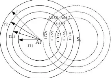
The basic 802.11 MAC layer uses the Distributed Coordination Function (DCF) to share the medium between multiple stations. DCF relies on CSMA/CA and optional RTS/CTS to share the medium. Due to the limitation of DCF, there is one station which “wins” the access to the medium can use the channel at the same time. Hence, the participation of the relay node may occupy larger range of area and keep the medium in that area from being accessed by other stations. Additionally, the hidden terminal problem (introduced by [13]) may happen due to the extended sensing area caused by the participation of the relay node as indicated by Fig. 1-2.

Figure 1-2 The extended sensing area

1.2 Motivation

In cooperative networks, the relay selection scheme affects a lot to the performance. In the last few years, several articles have been devoted to the study of the relay selection scheme. Although a large number of studies have been made on this issue, most relay selection methods aim to select the relay node by measure the communication state with the

(11)

source and destination. Actually, it just only needs to meet certain quality of the communication state to do with the cooperative communication. Besides successfully accomplishing the cooperation communication, maybe we could improve the spatial channel reuse by choosing the relay node within the area which has less contention for accessing the transmission medium.

1.3 Organization

The remaining of this thesis is organized as follows. Chapter 2 describes the related work including the cooperative communication MAC protocols with the relay (partner) selection schemes. In chapter 3, the proposed relay selection scheme and the corresponding MAC protocol are described in detail. The simulation results will be introduced in chapter 4. Last, the conclusion and future works are in chapter 5.

(12)

Chapter2 Related Work

This chapter will introduce some cooperative communication MAC protocols and the associated relay (partner) selection methods. After introducing the cooperative MAC

protocols and the associated relay selection schemes, the following is the discussion of them.

2.1 Cooperative Communication MAC and the Associated Relay

Selection Schemes

For propose of enhancing the reliability and the robustness of the WLAN operation, a cooperative communication MAC [7] is proposed.

In this protocol, the partner (relay node) retransmits the MAC frame received from the source when the frame is received in error at the destination. That is to say, if an acknowledgement from the destination is not received in aSIFSTime after completion of receiving the data frame, the partner(s) that received the data frame correctly from the source shall transmit this frame.

This protocol may utilize more than one partner and thus the transmission by partner is governed by a random backoff process to resolve potential collision between partners. The protocol is shown in Fig.2-1.

The partners shall always choose their backoff time within [0, CWp] for transmitting

other nodes’ frames regardless of the retransmission result. The value of CWp is announced by

the AP in its beacon based on the number of associated stations. In ad hoc wireless networks, the nodes choose CWp = CWmin .

Each node requires two MAC queues with the first queue being the data queue for its own outgoing data and the second queue, called partner queue that keeps the copy of the

(13)

currently transmitted frame that has not been acknowledged by the destination.

Figure 2-1 Basic CMAC protocol

The paper [8] proposed a cooperative MAC protocol with a rate sensitive relay selection scheme. Several rate adaptation algorithms, which are used to choose the optimal rate, have been proposed in 802.11 systems. These rate adaptive algorithms like Auto Rate Fallback (ARF) [9] and Receiver Based Auto Rate (RBAR) [10] may choose different modulation schemes according to the performance of the transmission quality or the communication state information. In this protocol, the physical modulation scheme is not changed between nodes during the transmission period. But packets are transmitted at different rates depending on the

(14)

distance between the source and the destination.

Figure 2-2 Cooperative regions for CoopMAC

In this protocol, the source will decide the dedicated helper (relay node) by observing the rate used for transmission between neighbor nodes. Each station maintains a table, called the CoopTable, of potential helpers that can be used for relaying data during transmission. The CoopTable contains the following fields: (1) the ID field, which stores the MAC address of the potential helpers. (2) The Time field, which stores the time of the last frame transmission heard from this node. (3) The Rhd field, which stores the data rate from the helper to the

destination. (4) The Rsh field, which stores the data rate from the source to the helper. (5) The

NumOfFailures field, which records the sequential failures associated with the helper.

With the Rhd and Rsh, the needed time to accomplish the two hop transmission is able to

be calculated. In the RTS/CTS mode, the condition for a cooperative transmission can be expressed as , 8 2 8 8 direct SIFS HTS PLCP hd sh R L T T T R L R L ₊ ₊ ₊ ₊ _< (2.1)

Where is the data rate for a direct transmission from the source to the destination and , , and are the additional time with a helper-aided transmission for the overhead. The HTS is a new message used to inform the source and the destination that the

direct

R

PLCP

(15)

helper is available during the cooperative transmission time.

The source decides the helper by means of calculating the total transmission time by (1). The helper with the minimum transmission time will be selected.

Figure 2-3 Control frame and Data frame exchange in CoopMAC

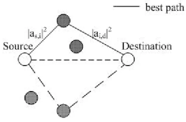
The paper [11] proposed a scheme that selects the best relay between the source and destination based on instantaneous channel measurements. This communication scheme exploits the wireless channel at its best, via distributed cooperative relays, is called

opportunistic relaying.

(16)

A single relay among a set of M relay nodes is selected, depending on which relay node provides for the “best” end-to-end path between the source and destination. As Fig. 2-4 indicates, the wireless channel asi between the source and each relay i, as well as the channel

aid between relay i and destination affect performance. The channel estimates asi, aid at each

relay, describe the quality of the wireless path between source-relay-destination, for each relay i.

Since the two hops are both important for end-to-end performance, each relay should quantify its appropriateness as a relay, using two functions that involve the link quality of both hops. The two functions are: under policy I, the minimum of the two is selected (equation (2)), while under policy II, the harmonic mean of the two is used (equation (3)). Policy I selects the “bottleneck” of the two paths while Policy II balances the two link strengths and it’s a smoother version of the first one.

} | |, | min{| 2 2 id si i a a h = (2.2) 2 2 2 2 2 2 | | | | | | | | 2 | | 1 | | 1 2 id si id si id si i a a a a a a h + = + = (2.3)

The relay i that maximizes function hi is the one with the “best” end-to-end path between

the source and destination.

(17)

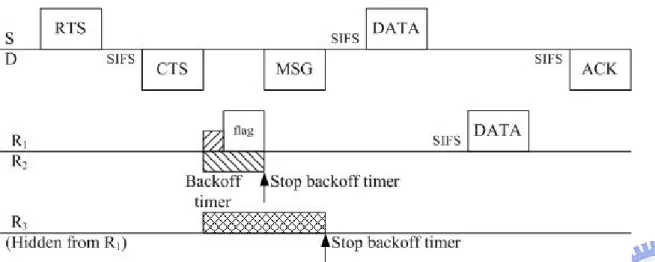
As Fig. 2-5 indicates, the relay nodes overhear a single transmission of a Ready-to-Send (RTS) packet and a Clear-to-Send (CTS) packet from the destination. The transmission of RTS from the source allows for the estimation of the instantaneous wireless channel asi

between the source and the relay i. Similarly, the transmission of CTS from the destination, allows for the estimation of the instantaneous channel aid between relay i and the destination.

As soon as each relay receives the CTS packet, it starts a timer from a parameter hi based on

the instantaneous channel measurements asi, aid. Each relay i will start its own timer with an

initial value Ti, inversely proportional to the channel quality hi, according to the following

equation:

i i

h

T = λ , (2.4)

where λ is a constant. The units of λ depends on the units of hi. Since hi is a scalar,

λ has the units of time. In this work, λ has simply values of μsecs.

2.2 Discussion

There’re other relay selection schemes based on location information with respect to source and destination. The idea was suggested by [12]. But such schemes require knowledge or estimation of distances between all relays and destination.

In CMAC, it proposed a method that all the source and partners randomly backoff to contend for relaying the data. The relay selection scheme is out of its concern. Although the relay is randomly decided, the concept of all source and relays contending for relaying is inspiring and relay only when the first transmission fails to reduce the retransmission times is reasonable. The scheme that relay after failed in the first transmission is adopted in our cooperation MAC scheme.

(18)

candidates to contend for relaying. But each relay will start its own timer with a value according to the instantaneous channel state between itself, source and destination. The relay selection scheme is not random backoff but determined by the channel measurement. Opportunistic relaying only considers the end-to-end channel state in the source-relay-destination path. But neighbor traffic is not taken into consideration.

In CoopMAC, every station observes the rate used among the neighbor stations to select the best relay which has the highest rate in this source-relay-destination path. This method selects the relay node actually corresponding to the end-to-end channel state. The rate to be used depends on the channel state measurement between the source and destination. An approach similar to CoopMAC called rDCF was proposed in [13]. The rDCF protocol enables packet relaying in the ad hoc mode of 802.11 systems by requesting each station to broadcast the rate information between stations. With the rate information, the cooperative MAC and the relay selection scheme is similar with CoopMAC. The MAC in this thesis is similar with CoopMAC but with different relay selection scheme and the relay retransmit the packet only when the first transmission fails. The comparison of relay selection schemes is in Table 2-1.

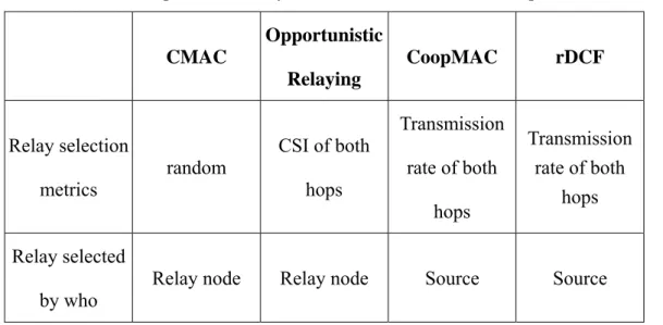
Table 2-1 Comparison of relay selection schemes in different protocols

CMAC Opportunistic Relaying CoopMAC rDCF Relay selection metrics random CSI of both hops Transmission rate of both hops Transmission rate of both hops Relay selected by who

Relay node Relay node Source Source

In the next chapter, the relay selection scheme with maximizing channel reuse will be proposed.

(19)

Chapter3 NAV-based Relay Selection

Scheme

In this chapter, we introduce our proposed cooperative node selection scheme, named NAV-based relay selection (NAV-RS) scheme. NAV-RS consists of two phases: information gathering and relay node selection. Information gathering is to construct and update maintained table. Based on the recorded information, relay node selection is for a source node to select the best relay among all candidates to improve its transmission efficiency.

3.1 Information Gathering

We assume each mobile station broadcasts Hello messages periodically, and the channel state information (CSI) between two nodes can be obtained from received signals.

To support cooperative communications, each mobile host maintains a neighbor table. This neighbor table contains four fields: node ID, SNR value, NAV value, and last update time, as shown in Fig.3-1.

Figure 3-1 Data structure of a neighbor table

The first column in Fig. 3-1, the Node ID field, stores the MAC address of the neighbor. The

SNR field stores the SNR value between self and the neighbor. The SNR value is calculated

by ) _ _ _ log( 10 ₁

∑

− + ⋅ = _i i Power Rx Noise Power Rx SNR , (3.1)

(20)

where Rx_Power is the frame signal strength at the receiver. It is calculated by the

propagation model. Noise_ is calculated from the receiver sensitivity of the data rate used by the frame. is the sum of the signal strength of the frames transmitted at the

same time. The NAV field stores the NAV value which is updated by receiving hello messages. The last field in the table, Last update field, stores the time of the last hello message

transmission heard from this neighbor.

∑

i−1 _

i

Power Rx

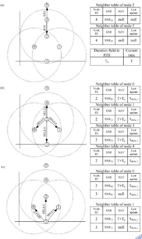
To take an example to illustrate information gathering, it is shown in Fig. 3-2. In Fig. 3-2 (a), node 2 and node 5 update the SNR values in the SNR field of the neighbor table after

receiving the RTS frame transmitted by node 4. Besides, node 2 and node 5 update its own NAV value with the sum of T and Td, where T is the time when finishing receiving the RTS

frame and Td is the duration time contained in the RTS frame. After that in Fig. 3-2 (b), when

node 2 prepares to broadcast a hello message, it calculates the value of NAV duration which will be contained in this hello message by subtracting the current time from its own NAV value. As a result, after receiving the hello message, nodes can update their NAV values in the

NAV field of neighbor tables by the value of NAV duration contained in the hello message and

the last update time. In Fig. 3-2 (c), node 3 broadcasts its hello message with the value of NAV duration of this message to be set zero.

(21)

(22)

3.2 Relay Node Selection

With the needed relaying information of relay candidates, we can choose the best relay station for our purpose – maximizing the spatial channel reuse. The selection scheme is separate to two phases:

(1) Relay candidate determination:

Before we select the best relay, which nodes can be the candidates should be determined. We assume that the value of SNR between the relay candidate and the source shall be higher than the cooperative threshold. Let S be a set of all neighbor nodes. The set of candidates is

(

SNR SNR SNR SNR

)

r S r _sr > _threshold ∩ _rd > _threshold ∈

∀ ( ) ( ), , (3.2)

where and are SNR values between the source and relay candidate and the relay candidate and destination, respectively. It is indicated that [18], when the wireless channel is in the good state, the corresponding SNR at each time instant is taken from a uniform distribution in the range of 15 to 30dB, and when the wireless channel is in the bad state, the SNR value is drawn from the range of 0 to 15dB. In this thesis, the threshold is set to be 15.

sr

SNR SNR_rd

(2) Relay node selection rules:

(a) rule 1: – select the station which its value of SNR is the highest.

(b) rule 2: – select the station which its value of NAV in the neighbor table not exceeds the current time. If more than one relay candidate meets this condition, choose the station with the most recent update time corresponding to the last update time in the neighbor table.

If none of relay candidates is selected, the original 802.11 MAC (the direct transmission scheme) is used.

(c) rule 3: - select the station which its Loading is the lowest. In this thesis, rule 2 is used in the relay selection scheme.

(23)

For example, in Fig. 3-2, it is assumed that node 0 wants to transmit data frames to node 1 in cooperative mode and the relay candidates are node 2 and node 3. In our NAV-based relay selection scheme, rule 2 above, the source selects the relay based on their NAV values in the neighbor table. The NAV value of node2 exceeds the current time and the NAV value of node 3 doesn’t, so we will select node 3 to be the relay.

3.3 Integration of NAV-RS and MAC protocol

The cooperative MAC algorithm is divided into three cases according to whether the relay node is selected or available.

3.3.1 Case 1 - The source has not found out relay or doesn’t need a relay

Figure 3-3 802.11 MAC with Direct transmission

The first case is that there’s no relay candidate selected by the source node based on the relay selection scheme. As Fig. 3-3 indicates, the source sends the RTS (Request-To-Send) frame and waits for the CTS (Clear-To-Send) frame from the destination. After received the CTS frame, the source transmits the data frame directly to the destination. If the destination receives the data frame successfully, it sends the acknowledgement back to the source.

The same with IEEE 802.11 MAC, the source start random backoff to restart the transmission scheme if not received the expected ACK. The source will also restart the relay selection scheme to choose a relay node.

In this case, the source may not need a relay node to transmit the data frame if the

(24)

relay node when the channel state is bad. For example, in Fig. 3-2, the transmission between node 4 and node 5 doesn’t need a relay and transmit the data frame directly.

3.3.2 Case 2 - The source has selected a relay

Figure 3-4 Cooperative MAC with two hop transmission

In case 2, there’s a relay candidate selected to be the relay node (helper). Therefore, the number of times to transmit the data frame may be two. One for the first transmission by the source and the other transmission is done by the relay node if the first transmission fails.

At the beginning, the source node sends the RTS message which carries the MAC address of the designated relay node to the destination. The duration field of this RTS frame is set to be TRCTS + TCTS + TDATA + TACK + 4TSIFS, where TRCTS is the transmission time of a

RCTS frame, TCTS is the transmission time of a CTS frame, TDATA is the transmission time of a

DATA frame and TSIFS is a SIFS (Short Interframe Space) duration time.

After receiving the RTS message, the destination determines whether the request is in cooperative mode or not by checking to see if there exists a MAC address of the relay node. If

(25)

there existed a MAC address of the relay node, the destination will wait for the RCTS message sent by the relay node. Through this RCTS message, the destination node knows the relay node is available and replies a CTS message with the duration field set to be 3TSIFS +

2TDATA + TACK. Then, the source node transmits the DATA frame in a SIFS duration time after

receiving the CTS message.

As Fig 3-4 indicates, this case is separate to two minor cases: (a) the source transmits the DATA frame successfully in the first transmission and (b) the first transmission fails and the relay node transmits the DATA frame again to the destination. That is to say, if the DATA frame successfully received by the destination in the first transmission, it will reply the ACK frame to the source. Otherwise, the relay node detects that the first transmission fails when not overhearing the acknowledgment transmitted by the destination and transmits the DATA frame after a SIFS duration time. When receiving the DATA frame, the destination knows the DATA frame is transmitted by the relay node by means of checking if the MAC address of the source node is carried in the MAC header of this DATA frame. Finally, the destination will reply the ACK frame to the source.

For example, in Fig. 3-2, the transmission between node 0 and node 1 needs node 2 or node 3 to be the relay. If node 0 transmits data frames to node 1 successfully, the selected relay will discard the data frame overheard from node 0.

(26)

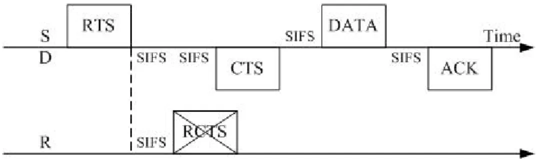
3.3.3 Case 3 - The source has selected a relay without responses of relay

Figure 3-5 Cooperative MAC with Direct transmission

This case is for the dedicated relay node is unavailable during this period of time. If the destination doesn’t receive the RCTS message, it will reply the CTS message back to the source in a SIFS duration time. Then the source transmits the DATA frame in a SIFS duration time. The destination replies the ACK frame back to the source if it has received the DATA frame. The source will restart the transmission scheme with relay node selection if it has not received the ACK frame.

For example, in Fig. 3-2, the transmission between node 0 and node 1 needs a relay and node 2 is selected to be the relay. Unfortunately, node 2 can’t transmit RCTS message when overhearing the RTS message which require node 2 to be the relay.

(27)

3.4 An Example which Illustrates the Algorithm

The scenario of this example is depicted as Fig. 3-6. There are two connections: Flow 0-1 and Flow 4-5.

(28)

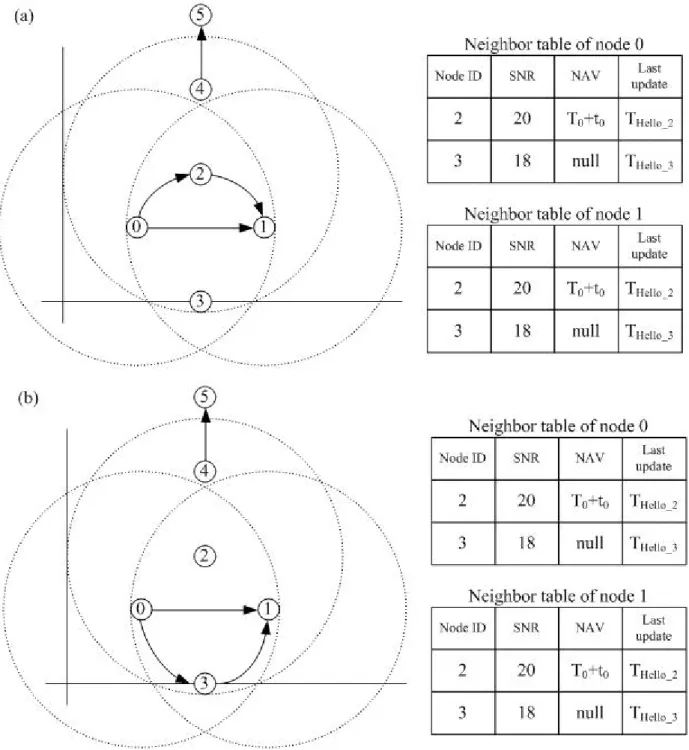
Figure 3-7 An illustration of the scheme to improve the spatial channel reuse

The assumption of this scenario is that the channel state information of Node 2 measured by Node 0 is better than that of Node 3 and the channel quality between Node 0 and Node 1 is too bad to complete the transmission by the direct transmission.

The result of this example may be different with different relay selection schemes. The description is divided into two cases:

In case 1, as illustrated by Fig. 3-7 (a), at the beginning, Node 4 sent a RTS message to the Node 5. Node 2 overheard this RTS message and set the NAV for the duration time of the transmission. Node 0 selected Node 2 as the relay only based on the channel state information of the source-relay-destination path. But Node 2 is blocked by NAV set by the RTS message transmitted by Node 4. Hence, Node 2 couldn’t help Node 0 to relay the DATA. As a result, only one transmission was successfully completed.

(29)

In case 2, as illustrated by Fig. 3-7 (b), at the beginning, Node 4 sent a RTS message to

the Node 5. Node 2 overheard this RTS message and set the NAV for the duration time of the transmission. In a short period of time passed, Node 2 and Node 3 broadcasted the short hello messages. The message transmitted by Node 2 contained the NAV information which is obtained from the duration field of the RTS message transmitted by Node 4. Based on the proposed NAV-RS, when Node 0 wanted to initiate the RTS message, Node 0 selected Node 3 other than Node 2 to be the relay node. Finally, the both two transmissions were transmitted successfully and the spatial channel reuse has been improved.

(30)

Chapter4 Performance Evaluation

In this chapter, the performance evaluations of 802.11 DCF, Opportunistic Relaying (OR) and Relay Selection based on NAV (NAV- RS) will be proposed by using ns-2 simulator [15].

4.1 Simulation Environment

The wireless channel model used in the simulation is “802.11b”. As a famous international standard for wireless local area networks, 802.11b uses different modulation schemes (BPSK, BPSK, QPSK, and CCK) which provide four physical layer rates ranging from 1 to 11 Mbps (1Mbps, 2Mbps, 5.5Mbps, 11Mbps).

The propagation model used is “TwoRayGround”. The two-ray ground reflection

model considers both the direct path and a ground reflection path. This model gives more accurate prediction at a long distance than the free space model. The received power at distance d is predicted by [15] L d h h G G P d P t t r t r r 4 2 2 ) ( = , (4.1)

where Pt is the transmitted signal power. Gt and Gr are the antenna gains of the transmitter and

the receiver respectively. L (L ≥ 1) is the system loss. Gt = Gr = 1 and L = 1. ht and hr are the

heights of the transmit and receive antennas respectively.

In this simulation, the error model used is based on [16]. This error model can be used to simulate wireless transmission error due to bad channel quality. It determines whether one frame is transmitted correctly by the BER which is obtained from the relationship between BER and SNR & Modulation. The relationship is indicated by Table 4-1, which is gotten from curves of Intersil HFA3861B specification [17]. Hence, SNR need to be calculated to get BER.

(31)

Table 4-1.Intersil HFA3861: The Relationship between BER and SNR & Modulation

SNR (dB) BPSK(1Mbps) QPSK(2Mbps) CCK5.5(5.5Mbps) CCK11(11Mbps)

5 5e-2 6e-2 4e-2 1.2e-2 6 5e-2 6e-2 1.3e-2 6e-3 7 1.2e-2 1.7e-2 4.1e-3 2e-3 8 4.1e-3 6e-3 1.3e-3 7e-4 9 1.1e-3 1.7e-3 3.3e-4 2.5e-4 10 2.2e-4 4e-4 8e-5 8e-5 11 4e-5 6.3e-5 1.5e-5 2.7e-5 12 2.9e-6 8.9e-6 2.7e-6 8e-6 13 3.6e-7 1.3e-6 5e-7 1.9e-6 14 4e-8 2.7e-7 5e-8 3.9e-7 15 3e-9 4e-8 1e-8 1.02e-7 16 1.8e-10 4e-9 1.1e-9 3e-8 17 1.8e-10 4e-9 1.1e-9 4e-9

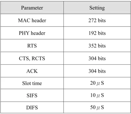
In this simulation, the system is heavily loaded. There are three different scenarios. The parameters based on the specification of Orinoco 11b card in this simulation are showed in Table 4-2.

Table 4-2.Parameters used in this simulation Parameter Setting MAC header 272 bits

PHY header 192 bits

RTS 352 bits CTS, RCTS 304 bits ACK 304 bits Slot time 20μS SIFS 10μS DIFS 50μS

(32)

4.2 Performance Metrics

The performance metrics measured in the simulation include the network throughput, service delay, transmission times, loss rate, and transmission cost as defined below:

A) Network throughput (KB/sec)

The summation of the packet sizes in all flows in a given period of time. B) Service delay (s)

The time duration from when the packet becomes the Head-of-Line packet in the buffer till it leaves the system. In this simulation, the service delay is the time duration from when the source start to send the RTS message till the destination receives the data. Besides, the service delay is the average delay of all received data frames. The lost data frame will not be considered to calculate the mean service delay in a given period of time.

C) Transmission times

The times that the source transmits the data to the destination, includes the first transmission and the retransmission times if the transmission fails.

D) Loss rate

The received data packets to the total generated packets ratio. E) Transmission cost (s)

The time duration that the medium is occupied by a successful transmission no matter how many times of the retransmission

F) Throughput gain (%)

(33)

4.3 Simulation Result

In the first scenario, the number of stations is six. Each station has no mobility. There is one traffic connection between Node 0 and Node 1 (flow 0-1) and another traffic connection between the Node 4 and Node 5 (flow 4-5). The max number of packets which arrive at the flow 4-5 is 10000. Packets arrive at each connection at a rate of 200 packets/sec and each MSDU packets is 512 bytes in length. This scenario is depicted in Fig. 4-1.

The simulation result is the average of results in 5 runs in which the distance between the Node 0 and Node 1 varies. In these runs, the distance between the Node 0 and Node 1 is far, so the connection of the two nodes needs a relay node to help relay the data. Otherwise, the performance of this connection may get worse due to the high error rate. Besides, the location of Node 2 is more closely to Node 0 and Node 1 than Node 3.

In the following simulation, the opportunistic relaying (OR) will be compared with the proposed relay selection scheme based on NAV (NAV-RS) and different lengths of hello message interval will be used. For example, NAV-RS _0.01 expresses that the proposed relay selection scheme based on NAV which the length of hello message interval is 0.01 second.

(34)

Figure 4-2 Service Delay of 802.11 vs. OR vs. NAV-RS with different hello message intervals

Figure 4-3 Throughput of 802.11 vs. OR vs. NAV-RS in different hello message intervals

We observed the impact of “hello message” frequency on service delay and throughput. As indicated by Fig. 4-2 and Fig.4-3, when the hello message internal is short as 0.01 seconds, it may cause more collisions and waste more channel usage to transmit the hello message. As a result, the performance is worse. After increasing the length of hello message intervals, we can alleviate the overhead of hello messages, but when the lengths of hello message intervals

(35)

exceed 0.05 second, it reduces the accuracy of information obtained by hello messages. Thus, we adopt “0.05 second” as the length of hello message interval in the following simulations.

Figure 4-4 Service Delay of 802.11 vs. OR vs. NAV-RS in Scenario 1

As indicated by Fig. 4-4, when the time is at 50th second, the number of arrived packets of flow 4-5 reached 10000. As a result, the effect caused by the flow 0-1 is gone. The delay decreases in the opportunistic relaying and NAV-RS. But, the influence affected by the flow 4-5 is lower in the proposed NAV-RS. This is because NAV-RS not only selects the relay which can help relay the data but also considers whether the relay candidate is appropriate or not to help relay the data. In this scenario, the opportunistic relaying is more likely to select Node 2 with the relay node because of the better channel quality in the path 0-2-1 due to the location of Node 2 and Node 3. On the other hand, in the proposed NAV-RS, the times to select Node 3 to be the relay node is less because the dense traffic near Node 3 leads the hello message sent by Node 3 will more likely to carry with the NAV information to prevent being selected for relaying.

(36)

Figure 4-5 Throughput of 802.11 vs. OR vs. NAV-RS in Scenario 1

From Fig. 4-5, it can be showed that the performance of throughput in our relay selection scheme outperforms that in opportunistic relaying scheme and the performance of throughput with cooperative communication is better than that in 802.11. The decreasing of throughput at about 50th second is because of that the number of arrived packets of flow 4-5 reached 10000 and no packets arrived at the flow 4-5. After about 50th second, the throughput is equal to the throughput of the flow 0-1. The reason for that the proposed NAV-RS outperforms than opportunistic relaying (OR) is the same as the reason for the performance of Service delay which is discussed.

(37)

Figure 4-6 Flow 0-1’s throughput of 802.11 vs. OR vs. NAV-RS in Scenario 1

As indicated by Fig.4-6, the performance of throughput in OR is worse than NAV-RS because of the flow 4-5 before the 50th second.

(38)

The number of the average transmission times in our method is lower than the average transmission times in the opportunistic relaying scheme and 802.11 indicates that the probability to successfully transmit the data is higher in the proposed NAV-RS. In our method, the sender is more likely to select the relay node which is not interfered by other traffics.

Figure 4-8 Loss rate of 802.11 vs. OR vs. NAV-RS

Figure. 4-8 shows that in the proposed NAV-RS, the loss rate is very low while the loss rate is increasing in the opportunistic relaying and 802.11. This is because the impact of the neighbor traffic.

(39)

Figure 4-9 Transmission cost of 802.11 vs. OR vs. NAV-RS

In Fig. 4-9, it shows the transmission costs of different protocols. The transmission cost in the worst case of 802.11 is lower because it doesn’t use the cooperative communication. But in the average, the transmission costs in 802.11 and opportunistic relaying (OR) are both higher than that in the proposed NAV-RS. Both using cooperative communication, the performance of NAV-RS is better than that of opportunistic relaying.

(40)

In the second scenario, the number of stations is six. There is one traffic connection between Node 0 and Node 1 (flow 0-1) and another traffic connection between the Node 4 and Node 5 (flow 4-5). Packets arrive at each connection at a rate of 200 packets/sec and each MSDU packets is 512 bytes in length. Different from the first scenario is that Node 1 is near Node 0 at the beginning and moves away from Node 0 at a speed of 4m/sec. So, the communication state of flow 0-1 will get worse with the increasing distance between the two nodes .This scenario is depicted in Fig. 4-10.

(41)

Figure 4-11 Service Delay of 802.11 vs. OR vs. NAV-RS in Scenario 2

In Fig.4-11, at 87th second, the mean service delay increased rapidly. This is because the long distance between Node 0 and Node 1 causes the attenuation of the power and the SNR is too low to transmit packets directly. It’s about the time to start the cooperative mode. Otherwise, the high error rate may cause the data be dropped frequently. We are showed that the cooperative mode is activated and the performance differs.

The opportunistic relaying scheme may be affected by the other connection causing the delay being higher than that in our proposed relay selection scheme.

(42)

As indicated by Fig. 4-12, the performance of our proposed NAV-RS is the most stable and better than OR and 802.11.

(43)

0 0.5 1 1.5 2 2.5 3 3.5 4 4.5 4 12 20 28 36 44 52 60 68 76 84 92 100 108 116 Time(s) T ra ns m is si on tim es 802.11 OR NAV-RS

Figure 4-14 Transmission times of 802.11 vs. OR vs. NAV-RS in Scenario 2

Fig. 4-14 shows that the transmission times in our proposed NAV-RS is much lower than that of opportunistic relaying and 802.11. The result is corresponsive to the result of loss rate.

(44)

0 0.2 0.4 0.6 0.8 1 1.2 0 16 32 48 64 80 96 11 Time(s) L oss rat e 2 802.11 OR NAV-RS

Figure 4-15 Loss rate of 802.11 vs. OR vs. NAV-RS in Scenario 2 As showed in Fig. 4-15, in the proposed NAV-RS is about to have no loss.

(45)

In the third scenario, there are 10 nodes distributed in the simulation topology. There’s at least one connection needs the cooperation relay. The scenario is depicted as Fig. 4-17. We have several runs in this scenario with the packet size of 512 KB and 1024KB for each run.

Figure 4-17 Topology of Scenario 3

0 50 100 150 200 250 300 350 400 4 12 20 28 36 44 52 60 68 76 84 92 100 108 116 Time(s) T hr oughput (K B ) 512-802.11 512-OR 512-NAV-RS 1024-802.11 1024-OR 1024-NAV-RS

Figure 4-18 Throughput of 802.11 vs. OR vs. NAV-RS with different packet size In Fig. 4-18, we can see that no matter the packet size is big or not, the performance of throughput in our relay selection scheme is better.

(46)

Figure 4-19 Throughput gain of OR vs. NAV-RS

Through Fig. 4-19, it is showed that our relay selection scheme outperforms the opportunistic relaying scheme when there’s other traffic interfering. The opportunistic relaying select the “best” relay based on the instantaneous channel quality between the relay and the source as well as the quality between the relay and destination. But it doesn’t consider about the coexisting connection at the same time. The participation of the relay may affect other connections because the extended sensing area of the relay node. Besides, the transmission by the relay may be interfered by other traffics.

One may notice that with the increasing of the packet size, the improved percentage decreases in our method while increasing in opportunistic relaying. The possible reason is that as the overhead of the hello message in our relay selection scheme may collide with the transmission of data.

(47)

In the last scenario, there are 16 nodes randomly distributed in the simulation topology. There are 8 connections which are randomly set. The traffic type is CBR for each connection. The packet size is 512 byte and the rate is 512Kb per second. The simulation time is 50 seconds. All traffic are started at 1th second.

As indicated by Fig. 4-20, the performance of throughput in opportunistic relaying and NAV-RS are better than that in 802.11. The performance of throughput in OR and NAV-RS are similar. The possible reason may be that the location of nodes and connections are randomly set. As a result, sources could not find a better relay for them.

(48)

Chapter5 Conclusion and Future Work

At the beginning, the reasons that the wireless networks becomes popular is mentioned but unfortunately there’re still some limitations to the wireless network like the attenuation due to propagation and the fading caused by the multi-path problem. After that, the cooperative communication is introduced which includes why the cooperative communication can help and how the cooperative communication works to improve the throughput and reliability.

Later, we focus on the relay (partner) selection scheme in MAC layer. Several cooperative protocols with relay selection scheme are introduced in related works. By studying the related works, it is observed that most proposed relay selection scheme aim to select the relay by measuring the instantaneous channel state information but rarely consider the interference of other coexisting traffics and the problem of the extended sensing area due to the participation of the relay. Thus, a relay selection scheme based on NAV which considers neighbor traffic of the relay is proposed. In the proposed relay selection scheme, the purpose is to select the relay which is less interfered by other traffic and is qualified to help relay the data.

Through the simulation by using the ns-2 simulator, we can see that the performance of throughput and delays in the proposed scheme are better than that in opportunistic relaying and original 802.11 in some scenarios. After observing the impact of the frequency of hello messages, we have chosen a suitable value as the parameter of lengths of hello message intervals. In randomly distributed networks, sources may not find a better relay for them, but the performances are still better than that in original 802.11.

In the future work, we can do the mathematical analysis for the proposed scheme and the next step is to observer the relevance between the proposed scheme and the issue of hot spot avoidance.

(49)

Reference

[1] T Cover and AE Gamal, “Capacity theorems for the relay channel,” IEEE Trans.

Information Theory, vol. 25, pp. 572-584, 1979.

[2] A Sendonaris, E Erkip and B Aazhang, “User cooperation diversity. Part I. System

description,” IEEE Trans. Communications, vol. 51, no. 11, pp. 1927-1938, 2003.

[3] A Sendonaris, E Erkip and B Aazhang, “User cooperation diversity. Part II.

Implementation aspects and performance analysis,” IEEE Trans. Communications, vol.

51, no. 11, pp. 1939-1948, 2003.

[4] JN Laneman, GW Wornell and DNC Tse, “An efficient protocol for realizing

cooperative diversity in wireless networks,” Proc. IEEE Int. Symp 2001. Information Theory, pp. 294.

[5] TE Hunter and A Nosratinia, “Cooperation diversity through coding,” Proc. IEEE Int.

Symp 2002. Information Theory, pp. 220.

[6] TE Hunter and A Nosratinia, “Diversity through coded cooperation,” IEEE Trans.

Wireless Communications, vol. 5, no. 2, pp.283, 2006.

[7] NS Shankar, CT Chou and M Ghosh, “Cooperative Communication MAC (CMAC)-A

New MAC protocol for Next Generation Wireless LANs,” WirelessCom 2005. IEEE Int. Conf. vol. 1, pp. 1-6.

[8] P Liu, Z Tao, S Narayanan, T Korakis and SS Panwar, “CoopMAC: A Cooperative

MAC for Wireless LANs,” IEEE Journal on Selected Areas in Communications, vol. 25,

no. 2 pp. 340-354, 2007.

[9] A KAMERMAN and L MONTEBAN, “WaveLANR-II: A high-performance wireless

LAN for the unlicensed band: Wireless,” Bell Lab. Tech. J., vol. 2, no. 3, pp. 118-133,

1997.

[10] G Holland, N Vaidya and P Bahl, “A rate-adaptive MAC protocol for multi-Hop

wireless networks,” Proc. MobiCom 2001, pp. 236-251.

[11] A Bletsas, A Khisti, DP Reed and A Lippman, A., et al., “A Simple Cooperative

Diversity Method Based on Network Path Selection,” IEEE Journal on Selected Areas in Communication, Special Issue on 4G, January 2005.

[12] B Zhao and MC Valenti, “Practical relay networks: a generalization of hybrid-ARQ,”

IEEE Journal on Selected Areas in Communications, vol. 23, no. 1, pp. 7-18, 2005.

[13] H Zhu and G Cao, “rDCF: A relay-enabled medium access control protocol for wireless ad hoc networks,” IEEE Trans. MobiCom, vol. 5, no. 9, pp. 1201-1214, 2006. [14] AS Ibrahim and AK Sadek, “Cooperative communications with partial channel state

information: When to cooperate?,” GLOBECOM 2005. IEEE Int. Conf. vol. 5, pp. 5.

[15] Kevin Fall and Kannan Varadhan, “The ns Manual,”

http://www.isi.edu/ns/doc/index.html

(50)

[17] Intersil. HFA3861B: Direct Sequence Spread Spectrum Baseband Processor. 2000. [18] D Qiao, S Choi and KG Shin, KG Shin, ” Goodput analysis and link adaptation for

IEEE 802. 11 a wireless LANs,” IEEE Trans. MobiCom, vol. 1, no. 4, pp. 278-292.