I-Shou University Institutional Repository:Item 987654321/776

全文

(1)義守大學管理研究所 Graduate School of Management I-Shou University 博. 士. 論. 文. On Investment Strategies of CPT-TSD 累積利望參階機遇凌越投資策略之研究. 指導教授：陳文魁研究生：曹耀鈞. 中華民國九十八年六月.

(2)

(3) 誌謝經過了數不清的白天與黑夜，博士論文終於順利完成且通過學位考試，首先要感謝的人，就是我的博士論文指導教授. 陳文魁博士，恩師治學嚴謹且親力親. 為的研究與教學態度總是令人動容。從論文的財務經濟理論模型推導、進以剖析相關浩瀚文獻脈絡、從而架構研究方法的創意、直至論文的程式技巧與寫作舖陳的掌握，皆有. 吾師深遠且直接的指點。不僅如此，在我博士課程的求學階段中，. 遇有令人沮喪挫折之瓶頸，老師總會適時地用堅忍但和藹的態度來勉勵我奮力渡過；在我偶有突破困境且自覺得意之際，他卻又會以充滿邏輯質疑的話語來適時地矯正我的不足之處。一如. 吾師教誨，在完成博士論文，取博士學位之時，才. 是正式研究的起點而已。所以在往後的學術生涯中，我一定會時刻提醒自己稟持著謙卑的態度在學術領域不斷地自我成長。國立中山大學財管系國立高雄第一科技大學風管系. 周建新教授、國立高雄應用科技大學金融所. 建衡教授、國立高雄餐旅學院旅管所授及義守大學財金系. 徐守德教授、. 鄭駿豪教授、義守大學企管系. 周崇輝教授六位. 杜. 葉兆輝教. 口試委員對耀鈞的厚愛與鼓勵、詳細審. 閱長篇論文並不厭其煩地給予真知灼見，是我的博士論文更瑧完備的重要推手。猶記在我學位考試正式宣布通過，接受. 口試委員一一祝賀之時，心中感激之情. 實在無以言語。管理學院. 林麗娟院長、. 彭台光副院長，您們對學術專業素養的有所堅持. 與毫不妥協，是我謹記效法的典範。本校. 黃俊英講座教授在我副修行銷博士課. 程時的引領與提點，如今仍然歷歷在目。另外，管研所. 許婷婷助理的行政長才. 真是不可多得，她處事的高效能與負責任的態度著實令人激賞難忘。她蘊細的佐助，讓我能更專心地進行博士論文的最後付梓，咸讓處於緊張時刻的我，得以因為她的行政協助而寬心許多。實踐大學. 張春雄講座教授對耀鈞多年來的慈愛與. 照拂，一直有增無減。母校東吳大學企管研究所. v. 蘇雄義教授對耀鈞的溫心關懷.

(4) 未曾間斷。還有，東吳大學商學院前院長. 何照義教授和企管系. 句句勉勵，我均字字牢記。此外，也要感謝台灣大學大學亞太所. 顧長永教授和成功大學社科中心. 劉美纓教授的. 財金系沈中華教授、中山. 蕭元哲教授在我攻讀博士過程中. 給我的正面評價，使我更有信心地完成博士學位。菲律賓 Ateneo 馬尼拉大學學術副校長 Dr. Antonette Palma-Angeles 及越南國家社科院中國研究所杜金森所長在我修讀博士期間，邀請我前往兩國作多日的實地財經研究，這樣深刻且具體的國際研究歷程絕對會是我一生難忘的學術經驗。正修科技大學校長的提攜之情及主任秘書. 龔瑞璋博士對我的知遇之恩、副校長. 吳正義教授于我. 李偉山博士的強力支持，他們對我的勉勵期許都還深植. 我心，更提供我良好的學術研究環境，讓我能安心深造而沒有經濟上的憂慮，這是我深深銘記感謝而不能或忘的。當然，正修科技大學企管系. 梁瑋傑老師是我. 多年來如同手足的摰友，我們每月在一起分享研究與教學心得的二人兄弟會，好似在緊湊的學術研究生活中的智識野宴，成為我學術研究過程的歡樂時光。還有，著名上市公司偉詮電子. 林錫琨董事、. 林錫銘董事長賢昆仲和亞東綜合證券. 蔡明秀協理，這些年來對耀鈞的賞識、厚愛如同家人，我常泉湧心頭。憶及義守大學財金所學妹. 高維琳在電腦程式的協助和我們共同研討時的專注情景，彼種. 形而上的知識匯聚，每每令人回味不已。除此之外，我的優秀學生白憶萱同學，也是我在學校的教學助理，她在教學材料的準備及相關課程輔助，實質減輕我不少的教學負擔，在此也要謝謝她的辛勤付出。最後，我要感謝自小栽培我的兩位小兒銘仁、銘宏的賢內助. 父母、呵護我的. 兄長們及悉心照料家務與. 靜雯，沒有你們無私的付出與愛心，我不可能完. 成這項艱鉅但值得傾力而為的任務。. vi.

(5) 摘要本研究運用累積利望理論 (CPT)與三階機遇凌越 (TSD)的方法，將交易所股票型基金 (ETF)50 檔成份股進一步作投資組合篩選。藉由本文所提出的累積利望三階機遇凌越模式 (CPT-TSD) ，遞減式絕對風險趨避型 (DARA)投資者可以獲得符合其最大效用的投資組合。本文所提出的擇股策略與資金配置技巧，可以在兼顧績效的前提下，有效降低投資組合數目。實證上，我們將交易所股票型基金的 50 檔股票，平均降低至只剩 4 至 5 檔股票，此舉大大地簡化投資組合的管理數目。機構投資者或基金經理人可以利用本研究所建議的方法來建構、評估例行性的投資組合配置，並且擁有較易管理、監控及降低交易成本的優點。本論文也以兩種無母數檢定，提出並驗證在四種選股策略模式下，四種相對應的資金配置戰術。本研究發現，若以月報酬為投資組合篩選的基礎，採用品累積利望三階機遇凌越模式策略搭配價格加權的資金配置戰術，績效表現最佳；若以週報酬為投資組合篩選的基礎，則以累積利望三階機遇凌越模式策略搭配平均加權的資金配置戰術，績效表現最好。值得強調者，本文乃目前學術文獻中，首先將 TSD 方法結合 CPT，體現兩者理論並實際應用於投資組合的第一篇研究。. 關鍵字：機遇凌越理論、累積利望理論、價值函數、機率加權函數 vii.

(6) Abstract This study employ the cumulative Prospect Theory(CPT) and Third Degree Stochastic Dominance(TSD) approaches to rank the performance of component stocks in Exchange Traded Fund 50. By constructing CPT-TSD portfolios, Decreasing Absolute Risk Aversion (DARA) investors can be guaranteed maximize their utilities but not their wealth achieves. In this paper, CPT-TSD iterations reduced a large number of stocks (50) into a manageable handful (nearly 4 to 5), greatly simplifying portfolio selection. Institution investors or fund managers could use this method to construct their portfolio with advantages of easy-supervised numbers and trading cost-down. Some evidence of stock picking ability among various portfolio strategies has also been found in the ranking priority test. Certainly, the recommended weighted method was investigated and four weighted tactics were ranked pair-wised. CPT-TSD strategy with price weighted or equal weighted depends on monthly return sorting basis or weekly return sorting basis are examined in detail for pursuing the best strategy-tactics fitness. In addition, the paper is the first attempt to integrate TSD method into CPT foundation in portfolio literature.. Keywords: Stochastic Dominance Theory; Cumulative Prospect Theory; Value Function; Probability Weighting Function. viii.

(7) Content 1. Introduction ...........................................................................1 2. Utility Assumption ................................................................5 2.1 Increasing Wealth Preference....................................................... 6 2.2 Risk Aversion ............................................................................... 7 2.3 Skewness Preference (Ruin Aversion) ......................................... 8. 3. Stochastic Dominance .........................................................10 3.1 First Order Stochastic Dominance.............................................. 13 3.2 Second Order Stochastic Dominance ......................................... 14 3.3 Third Order Stochastic Dominance ............................................ 16. 4. SD in CPT............................................................................19 4.1 Prospect Theory .......................................................................... 19 4.2 Cumulative Prospect Theory ...................................................... 21 4.3 Cumulative Prospect Stochastic Dominance.............................. 24. 5. Data and Method .................................................................26 5.1 MV Criteria................................................................................. 26 5.2 CPT-SD Criteria ......................................................................... 28. 6. Empirical Results.................................................................41 ix.

(8) 6.1 Performance of Portfolios Sorted by Monthly Return ............... 41 6.2 Performance of Portfolios Sorted by Weekly Return................. 42 6.3 MV and CPT-TSD and ETF Index Portfolio Performance........ 44 6.4 Return Performance Rank .......................................................... 47 6.5 Portfolio Difference between MV and CPT-TSD ...................... 51. 7. Conclusions and Suggestions ..............................................53 References ...............................................................................58 Appendix A. The Proof of PSD Rule ..............................................................65 Appendix B. Complete MV Criteria Metric ....................................................68 Appendix C. Complete CPT-FSD Criteria Metric ..........................................78 Appendix D. Complete CPT-SSD Criteria Metric ..........................................88 Appendix E. Complete CPT-SSD Criteria Metric...........................................98 Appendix F. Portfolio Performance in Different Strategy.............................108 Appendix G. Portfolio Performance in Different Weighted Tactics .............159 Appendix H. Portfolio Difference Ratio........................................................167 Appendix I. Monthly Return Performance Ranking......................................169. x.

(9) Table Content Table 5.1 Example MV Criteria Metric..............................................................................................27 Table 5.2 Sample CPT-FSD Test .......................................................................................................31 Table 5.3 Sample CPT-FSD Metric Test............................................................................................32 Table 5.4 CPT-SSD ............................................................................................................................33 Table 5.5 Sample CPT-SSD Metric Test............................................................................................34 Table 5.6 CPT-TSD............................................................................................................................35 Table 5.7 Sample CPT-TSD Metric Test ...........................................................................................36 Table 6.1 Performance of Portfolios Sorted by Monthly Return in Different ....................................42 Table 6.2 Performance of Portfolios Sorted by Weekly Return in Different......................................43 Table 6.3 MV and CPT-TSD and ETF Index Portfolio Performance , 2003-2008 ............................45 Table 6.4 MV and CPT-TSD and ETF Index Portfolio Performance , 2003-2008 ............................46 Table 6.5 MV and CPT-TSD and ETF Index Portfolio Performance , 2003-2008 ............................47 Table 6.6 Return Performance Rank (Monthly Return Sorted) ..........................................................49 Table 6.7 Return Performance Rank (Weekly Return Sorted) ...........................................................50 Table 6.8 Portfolio Difference Between MV and CPT-TSD..............................................................52. xi.

(10) Figure Content Figure 5.1 Example MV Criteria Scatter Chart .................................. 28 Figure 5.2 CPT-FSD Dominant .......................................................... 31 Figure 5.3 CPT-SSD Dominant .......................................................... 33 Figure 5.4 CPT-TSD Dominant .......................................................... 36 Figure 5.5 Research Design ................................................................ 40. xii.

(11) 1. Introduction Active management is the art of stock selecting and market timing. Passive management refers to a buy-and-hold approach to portfolio management. With respect to market behavior there are, at the extremes, two views. At one extreme is the efficient market hypothesis which insists that the prices are always fair and quickly reflective of information. According to this view, prices react to information slowly enough to allow some investors, presumably professionals, to systematically outperform markets and most other investors. At the other extreme is the market failure hypothesis. A rather impressive group of investors worldwide believes it is difficult to beat markets and perhaps better not to try. Aside from these considerations of theory and evidence, there is a very practical advantage to passive management. For most asset classes there are long-time series of historical data that allow us to form reliable estimates of the risk of a given class and how closely the behavior of that class correlates with the behavior of other classes. Active management refers to a portfolio management strategy wherein the manager makes specific investments with the goal of outperforming an investment benchmark index. Ideally, the active manager exploits market inefficiencies by purchasing securities that are undervalued. Depending on the goals of the specific investment portfolio, active management may also serve to create less volatility than the benchmark index. The reduction of risk may be instead of the goal of creating an investment. return. greater. than. the. benchmark.. The. effectiveness. of. an. actively-managed investment portfolio obviously depends on the skill of the. 1.

(12) management. The most obvious disadvantage of active management is that the fund manager may make bad investment choices or follow an unsound theory in managing the portfolio. Malkiel (1999) advocated that there are rare to find exceptional financial managements. Actively managed mutual funds must strive to overcome this cost disadvantage by assiduously searching for and identifying investment opportunities that have the potential to generate above-average earnings and price appreciation. This highly competitive and daunting task is sufficiently demanding that the majority of equity funds have been unable to provide long-term performance superiority in comparison with the broad market. Moreover, those funds that dominate market averages in a specific time frame are typically unable to sustain outsized performance momentum in subsequent years. We can always hear the familiar announcement in a mutual fund prospectus that "Past performance is no guarantee of future results." On the other hand, passive management is a financial strategy to mimic the performance of an externally specified index. The concept of passive management is counterintuitive to many investors. It is widely interpreted as suggesting that it is impossible to systematically "beat the market" through active management, although this is not a correct interpretation of the hypothesis in weak form efficient market. In recent years, Exchange traded fund (ETF) has become a popular investment. It is an investment vehicle traded on stock exchanges and tracking the performance of specific indexes in the Stock Exchange. ETF replicates index stocks and it is a kind of passive management style. Therefore, it has the advantage of having the similar return as the indexes. ETF may be attractive because of their low costs, tax efficiency, and stock-like features. An ETF combines the valuation feature of a mutual fund or unit 2.

(13) investment trust. Contrarily, Bogle and Malkiel (2006) has argued that ETF represent short-term speculation, that their trading expenses decrease returns to investors, and that most ETFs provide insufficient diversification. Even though they concede that a broadly diversified ETF that is held over time can be a good investment. To conquer the disadvantages of active style and passive style management, we try to combine active operation into passive portfolio and figure out competitive performance and downsized managed to the bench market. Standard technical apparatus in these treatments has been Markowitz’s (1952, 1959) Mean-Variance (MV) framework. The MV model requires the asset returns to be normally distributed or the decision-maker’s utility function to be of quadratic form (Hanoch and Levy, 1969). For this reason, the reliability of performance comparisons using MV criterion depends on the degree of non-normality of the returns and the non-quadratic utility function (Fung and Hsieh, 1999). In many circumstances these assumptions appear questionable (see Markowitz, 1952, 1959; Sharpe, 1964). Hence the research question to be investigated is whether stochastic dominance analysis is capable of presciently divining those mutual funds that are more prone to reward investors with extraordinary returns. When the assumptions of MV do not hold, the Stochastic Dominance (SD) efficiency criteria offer the most immediate extension (Bawa, 1982; Levy, 1992). SD accounts for the entire probability distribution (not just the first two moments) and applies for the general classes of non-satiated and/or risk-aversive preference functions. The theory of stochastic dominance (SD) is consistent with expected investor utility maximization and involves no restriction on the class of investor utility functions. SD derives weak conditions for separation based on general probability distributions. Therefore, for rank-ordering portfolios based on their risk and return 3.

(14) trade-off, stochastic dominance is a general and powerful approach.For the argument between active and passive portfolio management, the purpose of our empirical exploration presented herein is to conduct an investigation of the efficacy of stochastic dominance theory in deducing an efficient subset of exchanges trade fund from a prohibitively large and unwieldy population. It is not my intention to see which portfolio performance is overwhelm outperforms one another. The aim of this study is to provide superior filter in both bull and bear markets as opposed to buy-and-hold strategy as traditional ETFs persist. The empirical exploration of the paper is to examine an intriguing and perplexing issue that continues to be debated in the investment analysis literature. Specifically, a familiar and prevalent tenet of contemporary portfolio theory is that the portfolios produced by mutual funds are only constructed from Mean-Variance trade off consideration. This highly competitive and daunting task is sufficiently demanding that the majority of equity funds have been unable to provide long-term performance superiority in comparison with the broad market. Moreover, those funds that dominate market averages in a specific time frame are typically unable to sustain outsized performance momentum in subsequent years. We also need to know if the CPT-TSD portfolio will sacrifice performance when we consider investors' S shape valuation function and probability weighting function. This observation does not preclude the prospect of discovering extraordinary performance by a sparse subset of portfolios. Hence the research question to be investigated is whether CPT-TSD is capable of presciently divining the broad market that is more prone to reward investors with competitive returns. This paper enables investors to make choices about allocations that concerns more about the macro issue 4.

(15) beyond the narrow micro-level study. This was one of the important topics that De Bondt , Shefrin and Staikouras(2008) suggested for future research. Besides, the paper examines the fitness of portfolio selection strategy and allocation tactics. Institutional investors or fund managers can adopt the recommended strategy-tactics on portfolio management. The rest of the paper unfolds as follows. The next section introduces the basic utility assumption linked to stochastic dominance notions. We then describe different class stochastic dominance method in Section 3. In Section 4, the characteristics of Stochastic in Cumulative Prospect Theory will be discussed. In Section 5, we discuss the sample data set and methodology. Section 6 is the empirical results and detail portfolio analysis. Following that is the concluding section, we puts forth some interesting routes for theoretical and practical improvement and future research extension as well.. 2. Utility Assumption The utility function measures the relative value that an investment places on a business outcome. Within this definition, however, lies a significant limitation of utility theory: we can compare competing options, but we cannot assess the overall acceptability of any of those options. In other words, there is not objective, absolute scale for utility. To specify a utility function we must have a measure that uniquely identifies each business outcome, typically some measure of profitability or terminal wealth, and a function that maps each business out come to its corresponding utility. By convention. 5.

(16) utility is purely an ordinal measure. In other words, utility can be used to establish the rank ordering of outcomes, but cannot be used to determine the degree to which one is preferred over the other. Any positive, linear transformation of a utility function will still yield the same rand ordering of investment alternatives. Unfortunately, we rarely know a priori what outcomes will result from various investment alternatives. Instead, forecasted terminal wealth has some distribution which varies depending upon the investment alternative selected. Classical utility theory assumes that rational investments seek to maximize their expected utility and choose among their investment alternatives accordingly. (Heyer, 2001) A is preferred to B if and onlyif terminalwealthsatisfies Ew [U (wA )] − Ew [U (wB )] ≥ 0. with at least one strictinequalityU (w A ) − U (wB ) ≥ 0.. ( 2.1). The utility function U reflects the risk/reward motivations of the investment. These same features also determine what stochastic characteristics the terminal wealth distribution must possess if one alternative is to be preferred over another. Evaluation of these stochastic characteristics is the basis of stochastic dominance analysis.. 2.1 Increasing Wealth Preference This feature captures the“more wealth is better” philosophy of investment behavior and is generally considered a universal feature of utility functions. For greater wealth to be preferred, the utility function must be monotonically increasing. A utility function possesses increasing wealth preference if and only if U ′(w) ≥ 0 for all w with at least one strict inequality.. 6. ( 2.2 ).

(17) 2.2 Risk Aversion This feature captures the willingness of an investment to pay more than the expected loss to transfer an insurable loss. This is a subset of increasing wealth preference; an investment may have increasing wealth preference with or without exhibiting risk aversion, and is also generally considered a universal feature of utility functions. A utility function possesses risk aversion if and only if it satisfies the condition for increasing wealth preference and U ′′(w) ≤ 0 for all w with at least one strict inequality.. ( 2 .3 ). It is not intuitively clear, however, that this mathematical definition of risk aversion is equivalent to the behavioral definition given above. To make this relationship clearer we must recognize that Equation 2.3 defines a concave function and apply Jensen’s inequality. E w [U (w)] ≤ U (E w [w]) Under risk aversion, then, the expected utility of a risky investment is less the utility of the expected outcome. Why should this be the case? By proposition the investment has penalized the utility of the investment for the possibility of unfavorable outcomes. If we rewrite Jensen’s inequality with a strict inequality as follows: E w [U (w)] = U (E w [w] − π ) This shows that the investment is indifferent between the return on a risky investment or a lower, risk-free wealth equal to E w [w] − π where π is the premium that the investment is willing to pay to eliminate risk.. 7.

(18) 2.3 Skewness Preference (Ruin Aversion) This feature is classically presented as an individual’s willingness to play the lottery: to accept a small, almost certain loss in exchange for the remote possibility of huge returns. An investment’s concern, however, is with the opposite situation, unwillingness to accept small, almost certain gain in exchange for the remote possibility of ruin. This is a subset of risk aversion; an investment may have risk aversion with or without exhibiting ruin aversion. Mathematically this is expressed as:. A utility function possesses ruin aversion if and only if it satisfies the condition for risk aversion and U ′′(w) ≥ 0 for all w with at least one strict inequality ( 2.4) As with risk aversion, it is not intuitively clear that the mathematical and behavioral definitions of ruin aversion are consistent. If we take a Taylor series expansion of the utility function about E w [w] , and take the expectation with respect to w, it is: U (w) = U (E w [w]) + U ′(E w [w]) ⋅ (w − E w [w]) +. U ′′(E w [w]) 2 ⋅ (w − E w [w]) 2!. U ′′′(E w [w]) 3 ⋅ (w − E w [w]) 3! U ′′(E w [w]) 2 U ′′′(E w [w]) ⋅σ w + ⋅ μ3 E w [U (w)] = U (E w [w]) + 2! 3!. +. ( 2.5 ). From this expression we can see that any investment feature that increases positive skewness μ 3 (or reduces negative skewness) acts to increase expected utility. Fishburn and Vickson (1978) assume that u (.) , the decision maker’s utility function is well-defined and finite over all possible outcomes. That is, if I is the 8.

(19) smallest interval such that all possible values of a measure of interest X take values in I , then u ( X ) is defined and finite on I , Also assume that X is bounded from below. Let U 1 be the class of utility functions whose member functions are strictly increasing. That is, U 1 = { u : u , u ′ are continuous and bounded on I , and u ′ > 0 on. I }. Here u ′ denotes the first derivative of the function u with respect to x and I. denotes the interior of the interval I . Decision makers with risk-seeking,. risk-neutral, or risk-avoiding preferences all have utility functions which are members of this class. Let U 2 be the class of utility functions whose member functions, in addition to being strictly increasing, are also concave. That is U 2 = { u : u ∈ U 1 , u ′′ is continuous and bounded on I , and u ′′ < 0 on I 0 }. Here u ′′ denotes the second derivative of the function u with respect to x . Decision-makers with risk-avoiding preferences have utility functions which are members of this class. Absolute risk aversion has been defined as Ra ( x ) = － u ′′( x ) / u ′( x ) whenever u ′ and u ′′ exist and u ′( x ) ≠ 0. For u ∈U 2 , Ra (x ) >0 ∀x ∈ I 0 .Although the second derivative is a measure. of curvature, it is not always a useful measure of risk aversion under utility scale changes of the form u ( x ) = au ( x ) with a > 0. Ra is, however, invariant under such scale transformations. Let U d = { u : u ∈ U 2 , R ′A ( x ) is continuous, bounded, and nopositive on I }. That is, U d is the class of utility functions whose member functions, in addition to being strictly increasing and concave, also exhibit decreasing absolute risk aversion (DARA).. 9.

(20) Let U 3 be the class of utility functions whose member functions, in addition to being strictly increasing and concave, also exhibit the characteristic that utility increases at a decreasing rate, the absolute value of which becomes smaller as x increases. That is, U 3 = { u : u ∈ U 2 , u ′′′ is continuous and bounded on I , and u ′′′ >0 on I 0 }, where u ′′′ denotes the third derivative of the function u with respect to x . Graphically, as u ′ > 0 and u ′′ < 0 tend to bend or curve the utility function from its initially rising trajectory back toward the horizontal, the effect of u ′′′ > 0 is to slow the rate of this bending. These are referred to as DARA utility functions. Decision makers with risk-avoiding preferences that also exhibit the characteristic that small gambles become more attractive (or at least do not become less attractive) as net wealth increases have utility functions that are members of this class. The DARA hypothesis is quite reasonable and appears to be widely accepted. The relations between stochastic dominance and the principle of maximization of expected utility are well known in the literature (see Huang and Litzenberger, 1988).. 3. Stochastic Dominance The objective of portfolio management is to restrain and confine investment choices into a subset of desirable and efficient assets discriminated from the population of investment candidates. An efficiency criterion is a decision rule that apportions the population of investment options into two mutually exclusive groups. The most widely known and applied efficiency criterion for evaluating investments is the MV model. The basic premise of financial optimization is that investors are rational, no satiating and risk averse. It is well known that MV model is consistent with this principle if either one of the following conditions is satisfied: 10.

(21) 1.. The rate of return of assets follows multidimensional normal distribution.. 2.. Utility function μ is quadratic.. The normality assumption is often used because it leads to tractable results. However, empirical studies of historical stock market returns do not support the normality assumption (Rosenbaum and Kariya, 1989). In addition, quadratic utility function has undesirable properties (Arrow, 1971). An alternative approach applies stochastic dominance analysis. SD ordering is widely-understood, with a growing set of applications in diverse areas such as economics, agricultural economics, finance, statistics, and operations research. There are four main areas of stochastic dominance development and application the researchers could donate: 1) theoretical development, 2) application of SD rules to empirical data, 3) application of SD rules to other economic and financial issues, and 4) application of SD rules in statistics (Levy, 1992). Besides, stochastic dominance method is based upon axiomatic treatment of risk, and it is widely accepted that this approach is superior to mean-risk analysis from the theoretical point of view. Many theoretical and applied contributions in these and related areas have been summarized by Mosler and Scarsini (1991), Levy (1992), Shaked and Shanthikumar (1994), Davidson and Duclos (2000), Muller and Stoyan (2002), Barrett and Donald (2003), Linton, Maasoumi and Whang (2005). Most of those studies examine the efficiency about portfolio construction. Few, if any, discuss about the stock performance under stochastic dominance selection versus bench market. Ogryczak and Ruszczynski (2002), Leitner (2005) and Wong and Ma (2006) emphasized that stochastic dominance approach is superior to Value-at-Risk (VaR) or conditional-VaR (CVar) approach. Recently, Gasbarro, Wong and Zumwalt (2007) utilized both the SD 11.

(22) approach and the CAPM criterion to compare the performance of 18 stock market indices and found that SD appears to be both more robust and discriminating than the CAPM in the ranking of stock market indices. To overview about stochastic dominance theory, let us consider two stationary time series of returns, Ri,t and Rj,t , t=1,2,…,T, with respective cumulative distribution functions (CDFs), Fi(r) and Fj(r), over the support r. The returns are not expected to be. iid, but can exhibit some dependency structures in the moments of the distribution. The null hypotheses that Ri,t stochastically dominates Rj,t, for various orders are as follows:. H1： (First order). Fi(r) ≤ Fj(r). H2： (Second order). ∫. H3： (Third order). ∫∫. H4： (Fourth order). ∫ ∫ ∫. r. Fi (t) dt ≤. 0. r. t. ∫. r. 0. Fi(s) dsdt ≤. 0 0. r. t. s. 0. 0. 0. Fj (t) dt. r. t. 0. 0. ∫ ∫. Fi (u) dudsdt ≤. Fj(s) dsdt. r. t. s. 0. 0. 0. ∫ ∫ ∫. Fj (u) dudsdt.. Mathematically, lower order dominance implies all higher order dominance rankings. In the case of first-order dominance, the distribution function of Ri, t lies everywhere at the right of the distribution function of Rj, t, except for a finite number of points where there is strict equality. This implies that for first-order stochastic dominance, the probability that returns of the ith asset are in excess of r, say, is higher than the corresponding probability associated with the jth asset. 12.

(23) Pr (Ri, t > r) ≥ Pr (Rj, t > r). (2.6). An important feature of the definitions of stochastic dominance is that they impose minimalist conditions on the preferences of agents within the class of von Neumann-Morgenstern utility functions that form the basis of expected utility theory. The different orders of dominance correspond to increasing restrictions on the shape of the utility function and the attitude towards risk of agents to higher order moments. These restrictions are non-parametric and do not require specific parametric functional forms. The relationship between the three stochastic dominance rules can be summarized by the following diagram: FSD → SSD → TSD, which means that dominance by FSD implies dominance by SSD and dominance by SSD in turn implies dominance by TSD. Stochastic dominance propositions are important contributions to the theory of portfolio choice. The theorems which define stochastic dominance are a direct reaction to and consequence of the various objections rose to using mean and variance alone to rank series of competitive opportunities faced by economic decision makers (Kjetsaa and Kieff, 2003).. 3.1 First Order Stochastic Dominance Let us begin with the definition of preference given in Equation 2.1 and the most general constraint on a utility function given in Equation 2.2, increasing wealth. 13.

(24) preference. We can integrate Equation 2.1 by parts to yield: E w [U (w A )] − E w [U (wB )] ≥ 0 ∞. ∞. ∫ U (t ) f (t )dt − ∫ U (t ) f (t )dt ≥ 0 A. B. −∞. −∞. ∞. ∫ U (t ) ⋅ [ f (t ) − f (t )]dt ≥ 0 A. B. −∞. U (t ) ⋅ [FA (t ) − FB (t )]. ∞ −∞. ∞. −. ∫ [F (t ) − F (t )]⋅ U ′(t )dt ≥ 0 A. B. −∞ ∞. ∫ [F (t ) − F (t )]⋅ U ′(t )dt ≥ 0 B. ( 3.1.1). A. −∞. By Equation 2.1 we know that U ′(w) ≥ 0 so for Equation 3.1.1 be true for all utility functions with increasing wealth preference we must have: A is uniformly preferred to B under increasing wealth preference (A dominates B by first - order stochastic dominance) if and only if [FB (w) − FA (w)]. ≥ 0 for all w. with at least one strict inequality.. ( 3.1.2 ). Especially, the FSD rule set no restrictions on the form of the utility function beyond the usual requirement that it be non-decreasing. Thus this criterion is appropriate for risk averters and risk lovers alike since the utility function may contain concave as well as convex segments. Considering its generality, the FSD permits a preliminary screaming of investment alternatives eliminating those alternatives which rational investment will ever choose.. 3.2 Second Order Stochastic Dominance Let us now use a stronger utility function constraint, risk aversion, to develop investment selection criteria. We begin with the definition of preference given in. 14.

(25) Equation 2.1 and the risk aversion given in Equation 2.3. We can twice integrate Equation 2.1 by parts to yield:. U ′(∞ ) ⋅. ∞. ∞. t. −∞. −∞. −∞. ∫ [FB (t ) − FA (t )] dt − ∫ U ′′(t ) ∫ [FB (u ) − FA (u )] dudt ≥ 0. ( 3.2.1). Since risk aversion is a subset of increasing wealth preference we know that U ′(∞ ) ⋅. ∞. ∫ [F (t ) − F (t )] dt B. A. is positive. By Equation 2.3 we know that U ′′(w) ≤ 0 so. −∞. for Equation 3.2.1 to be true for all utility functions with risk aversion we must have:. A is uniformly preferred to B under risk aversion (A dominates B by second - order w. stochastic dominance) if and only if. ∫ [F (u ) − F (u )]du ≥ 0 B. A. for all w with at least. −∞. one strict inequality.. ( 3.2.2 ). For second-order stochastic dominance (SSD), expected utility from holding asset i is generally greater than the expected utility form holding asset j, within the class of. utility functions with positive first derivatives and negative second derivatives u ′ ≥ 0, u ′′ ≤ 0. This class of agents is characterized by risk aversion, whereby a risk premium is needed to compensate investors from holding assets whose returns exhibit relatively higher volatility. The SSD is the appropriate efficiency criterion for all risk averters and their utility function are assumed to be concave. Therefore, the SSD is more applicable to real world investment than FSD.. 15.

(26) 3.3 Third Order Stochastic Dominance Whitmore (1970), Whitmore and Findlay (1978) expand the theory of stochastic dominance to third degree stochastic dominance. He attempts to construct a more efficient and restrictive decision rule by appending an additional assumption to the second degree stochastic dominance model. The new information relates to the contour of a utility function. The specific assumption posed is that investor’s exhibit DARA utility function. This assumption is attached to the second degree stochastic dominance supposition of risk aversion. Mathematically, this property mandates that the third derivative of an investor's utility function is positive. Absolute risk aversion measures the extent to which an investor is risk averse for a given level of wealth. As wealth increases more funds are invested in risky assets. It is generally agreed that most investors exhibit DARA. Alternatives A dominates Alternatives B according to third degree stochastic dominance if: Investors prefer more to less (the first derivative of the utility function is positive) and investors are risk averse (the second derivative of the utility function is negative) and investors exhibit DARA (the third derivative of the utility function is positive) and the sum of the sum of the cumulative probability distribution for all returns is never more with Alternatives A than Alternatives B and sometimes less (the distributions do not intersect). In decision situations we have to compare many alternatives. When alternatives take uncertain character we can evaluate the performance of alternatives only in a probabilistic way. In finance, problems arise with stock selection when we need to. 16.

(27) compare return distributions. The construction of a local preference relation already requires the comparison of two probability distributions. Furthermore, we use the definition of preference given Equation 2.1 and the ruin aversion definition given in Equation 2.4. We can thrice integrate Equation 2.1 by pares to yield:. U ′(∞ ) ⋅. ∞. x. t. ∞ ∫ [FB (t ) − FA (t )] dt − U ′′(x ) ∫ ∫ [FB (u ) − FA (u )] dudt −∞ L. −∞ ∞. −∞ −∞. w. L + ∫ U ′′′(w) ∫ −∞. t. ∫ [F (u ) − F (u )] dudtdw ≥ 0 B. ( 3.3.1). A. −∞ −∞. Since risk aversion is a subset of ruin aversion we know that:. U ′(∞ ) ⋅. ∞. x. t. ∞ ∫ [FB (t ) − FA (t )] dt − U ′′(x ) ∫ ∫ [FB (u ) − FA (u )] dudt −∞ ≥ 0. −∞. −∞ −∞. By Equation 2.4 we know that U ′′′(w) ≥ 0 , so for Equation 3.3.1 to be true for all utility. functions. with. ruin. aversion. we. must. have:. A is uniformly preferred to B under ruin aversion (A dominates B by third - order w t. stochastic dominance) if and only if. ∫ ∫ [F (u ) − F (u )] dudt ≥ 0 B. A. for all w with at least. − ∞− ∞. one strict inequality.. ( 3..3.2 ). The condition for third-order stochastic dominance (TSD) implies that the expected utility from holding asset i is generally greater than the expected utility from holding asset j, within the class of utility functions with positive first and third derivatives and negative second derivatives, 17.

(28) u ′ ≥ 0, u ′′ ≤ 0 , u ′′′ ≥ 0 . This class of agents increasingly prefers positively skewed. returns as they are prepared to trade off lower average returns for the chance of an extreme positive return (Ingersoll (1987) and McFadden (1989). The TSD rule is even much appropriate for investment. Unlike the risk aversion assumption of SSD, the TSD also assumes DARA. The population of risk averters with DARA is clearly a subset for all risk averters, and the TSD efficient set is correspondingly a subset of the SSD efficient set. Third Order degree stochastic dominance is often able to banish some investment prospects to the set of inefficient options that were unable to be banished by applying either of the preceding dominance models. This desirable outcome is not always possible, however. Sometimes no dominance at any level can be established-there is a breach in each of the three dominance rules. This is likely when multiple assets have performance histories which are sufficiently similar as to be incapable of being mathematically differentiated. Fourth-order stochastic dominance (FOSD) incorporates the fourth moment of the returns distribution. For fourth-order stochastic dominance of asset A over asset B , the expected utility from holding asset A is generally greater than the expected utility from holding asset B, for all utility functions with u ′ ≥ 0, u ′′ ≤ 0 , u ′′′ ≥ 0 , u ′′′′ ≤ 0. This class of agents is adverse to assets that exhibit extreme negative as well as positive returns. As agents prefer thinner-tailed distributions to fat-tailed distributions, to hold asses that exhibit the latter property they need to be compensated with higher average returns. Even where two assets exhibit the same volatility, the asset returns distributions may nevertheless exhibit differing kurtosis resulting in a risk premium between the two. 18.

(29) assets. Because the strict constraint of FOSD and excellent selection effectiveness TSD could achieved, it is rare to apply FOSD for financial investment. Although TSD is not as easy to interpret as first and second degree stochastic dominance; it is an important notion in the theory of stochastic dominance. Empirical investigations have shown that third degree stochastic dominance can significantly reduce the number of efficient, i.e. nondominated risky prospects as compared to second degree stochastic dominance (Schmidt and Trede, 2000; Schmidt,2005). Besides, Gotoh and Konno (2000) show portfolios on the efficient frontier are also efficient in the sense of third degree stochastic dominance.. 4. SD in CPT Kahneman and Tversky (1979, 1992) suggest Prospect Theory (PT) and Cumulative Prospect Theory (CPT) as an alternative paradigm to EU theory. They show that investors distort probabilities, make decisions based on change of wealth, exhibit loss aversion and maximize the expectation of an S-shaped value function which contains a risk-seeking segment. PT and CPT become a cornerstone in economic research and are the foundation of behavioral finance and behavioral economics (Levy, De Giorgi and Hens, 2003).. 4.1 Prospect Theory Prospect theory (PT) recently gained much popularity and there is stream of papers that build economic and financial model based on this theory. There have been many empirical and experimental attempts to test PT, most of which support the theory (Nadai and Pianca, 2007). 19.

(30) The four elements of PT are: 1.Investors evaluates assets according to gains and losses relative to a given reference point. 2. Investors dislike losses as compared to their liking of gains (loss aversion). 3. Value functions are S-shaped with turning point at the origin. 4. Probability assessments are biased that extremely small probabilities are over- valued. The latter point is known as probability weighting, which causes PT preferences to be inconsistent with first order stochastic dominance. This drawback has been solved with the CPT of Tversky and Kahneman (1992), which replaces the weighting of probabilities with that of the cumulative distribution functions (De Giorgi & Hens, 2006). In their original article Kahneman and Tversky (1979) suggest that in making decisions under uncertainty, the subject apply a monotonic transformation π (p) where p are the probabilities, and investors make decisions by comparing π (p) corresponding to the two distributions under consideration rather that by comparing the true probabilities, p , themselves. Previous work on PT in portfolio selection has mainly focused on the impact of loss aversion. Berkelaar, Kouwenberg and Post (2004) and Gomes (2005) have studied how loss aversion affects multi-period portfolio decisions. Barberis, Huang and Santos (2001) incorporate a dynamic reference point in a multi-period model with PT preferences. The model generates time varying risk premium, high mean and volatility for stock returns even if the underlying growth process has low variance. By contrast, the model generates portfolio strategies opposite to the disposition effect. Gomes (2005) studies a model with heterogeneous investors: a loss averted investor and a Constant Relative Risk Aversion (CRRA) investor. The shape of the utility function of the loss. 20.

(31) averted investor slightly differs from that suggested by Kahneman and Tversky (1979) and is concave also for large losses. The. Capital. Asset. Pricing. Model. (CAPM). is. derived. in. the. von. Neuman-Morgenstern (NM) expected utility framework, and because Expected Utility Theory (EUT) is experimentally criticized, the CAPM is indirectly also criticized. The NM expected utility framework (as well as most other economic models) assumes that investors are rational, and that they maximize expected utility. However, not all agree with these “rational investor” assumptions. The most well-known paradox of expected utility maximization was presented by Allais and Hagen (1979). In particular, in making choices between alternative uncertain prospects, individuals tend to distort the objective probabilities in a systematic manner, which may lead to the choice of an inferior investment and to wealth destruction. Kahneman and Tversky (1979) challenged the expected utility paradigm by suggesting PT as an alternative descriptive paradigm. PT is based on experimental findings regarding subjects` behavior and strictly contradicts the NM expected utility (Levy, De Giorgi and Hens, 2003).. 4.2 Cumulative Prospect Theory Tversky and Kahneman (1992) suggest that a transformation is done on the cumulative probability F rather than on probability p, namely, investors compare F*=T (F) and G*=T (G) where T is a monotonic non-decreasing transformation. T can be interpreted either as a misjudgment or as a subjective revision of probabilities which varies across investors. In such cases, even though all subjects observe the same pair of distributions F and G, the distributions F* and G* may vary across investors. Hence stochastic dominance may lose ground because each investor has his/her own 21.

(32) subjective feasible set; hence, in general each investor has his/her efficient set. In fact this is also true of the MV efficiency analysis introduced by Markowitz (1952). The reason for the disagreement between investors on F* and G* is that each subject may have his subjective transformation Ti (F) and Ti (G) where the subscript i corresponds to the i-th investor. Thus even if the objective feasible set is identical for all investors, the subjective feasible set (which is the relevant one for decision making) may vary among investors. In PT, a decision model where weights ω(p) rather than probabilities, p, are employed has three drawbacks: 1) it may contradict first-degree stochastic dominance (FSD), i.e. the monotonicity axiom, 2) the sum of the subjective probabilities, ω(p), may and up to more or less than 1, and 3) that decision weights, ω(p), technically cannot be applied to continuous distributions. To overcome these drawbacks, Tversky and Kahneman (1992) suggest that the subjects conduct a transformation of the cumulative distribution, rather than a transformation of the probabilities. They derive the CPT as a modification to PT, where the cumulative distribution functions are distorted. The other two components of PT mentioned above (basing decisions on change in wealth and the S-shaped value function) still hold in CPT. Behavioral research shows that CPT is much more successful in accommodating observed preferences (Baucells and Heukamp, 2006). CPT improves on the traditional expected utility framework and in empirical studies a substantial fraction of subjects show preferences among choices in a way that is in agreement with CPT.1 Loss aversion is mathematically expressed in CPT as a steeper value function in the losses domain, which captures the intuition that losses loom larger than gains. Loss aversion 1. See Bleichrodt and Pinto (2000) and Abdellaoui, Vossmann, and Weber (2003) for robustness test. 22.

(33) plays a central role in behavioral decision research (Langer and Weber (2001); Barberis, Huang, and Santos (2001). The S-shape of υ and one positive weighting function w+ and negative weighting function w+ are characteristics for CPT. Baucells and Heukamp (2006) advocate the stochastic dominance conditions are useful to design non-parametric test s of CPT. In sum, large families of modern descriptive theories of decision under risk depart from expected value maximization in three essential ways: the transformation of outcomes, the transformation of probabilities, and the composition rule that combines the two transformations. PT has emerged as the frontrunner of these descriptive theories (Starmer, 2000). In PT, outcomes are transformed by an S-shaped value function, concave for gains, convex for losses, and steeper for losses than gains; and probabilities are transformed by an inverse S-shaped probability weighting function, concave for small probabilities and convex for medium and large probabilities. A large body of empirical and theoretical investigation has supported these two aspects of PT. In contrast, the third aspect of PT, the composition rule, has received relatively little direct empirical attention. PT and CPT differ in how these two transformation functions are combined. CPT involves Rank Dependence Utility (RDU) in its valuation function formulation and fundamentally consists of two separate RDU representations for losses and gains. It has the attractive feature of generalizing diminishing sensitivity from probabilities to outcomes (Gonzalez and Wu, 2003). In fact, CPT has emerged as one of the most popular alternatives to EUT(Schmidt and Zank, 2008).. 23.

(34) 4.3 Cumulative Prospect Stochastic Dominance Levy and Weiner (1998) develop a dominance rule called Prospect Stochastic Dominance (PSD) corresponding to the S-shaped value functions. And they find a wide range of probability transformations under which the first degree, the second degree and the prospect stochastic dominance are intact. It is shown that SD rules are intact as long as some constraints are imposed on the transformations T (˙) of the cumulative probabilities: monotonicity of the transformation is required for FSD to be intact, monotonicity and concavity of T (˙) to keep SSD intact, and convexity of T (˙) for losses and concavity of T (˙) for gains to keep PSD intact (Levy and Levy, 2004). PSD include two ranges of outcomes; the negative and the positive ranges. The reason for this separate treatment of the two ranges is the inflection point in the preferences. For money outcomes, x = 0 is the inflection point. Let F and G be two stochastic investments with cumulative distributions F(x) and G(x), and let US denote the set of all S-shaped utility (or value) functions (U' 0 for all x. 0, U'' > 0 for x < 0, and U'' < 0 for x > 0). F dominates G for all U x. ∫ [G(t ) − F (t )]dt ≥ 0, y. Us iff. For all y ≤ 0 and for all x ≥ 0 with at least one strict. inequality. F dominates G by PSD if and only if the area enclosed between the two cumulative distributions G and F is positive for any range [y, x] with y. 0 and x ≥. 0. To introduce the intrinsic meaning of stochastic in CPT. We briefly derived the proof of PSD rule2 in Appendix A.. 2. See details in Lewandowski (2006). 24.

(35) CPT makes sure that the weight function is such that if there are two prospects, F and G., and if F dominates G by FSD, such dominance will be found also in PT framework. Thus, the transformation of cumulative probability does not violate FSD. Efficiency analysis of investments and in particular stochastic dominance partial ordering assumes homogeneity of expectations regarding the probability distribution. Experimental studies reveal that even if all investors observe the same distribution of returns, they perform a mental transformation of the cumulative distribution. In addition it is found that the utility function is S-shaped. Even though several other probability weighting functions have also been proposed, Cumulative Prospect Theory has gained a great deal of support as an alternative to Expected Utility Theory as it accounts for a number of anomalies in the observed behavior of economic agents.(See Lattimore, Baker, and Witte (1992), Prelec (1998)). Levy and Wiener (1998), Levy and Levy (2002, 2004) develop PSD corresponding to the S-shaped value functions. They find a wide range of probability transformations under which the first degree, the second degree and the prospect stochastic dominance are intact. Besides, Levy and Levy (2002, 2004) emphasize when subjective probability transformation is employed, portfolios that are PSD efficient with the objective probabilities may become inefficient. Later, De Nadai and Pianca (2007) note that previous preferences concern only the sign of the first and second derivative of the utility (value) function. He advocates researcher could build a stochastic indicator of the decision maker preferences which is progressively weaker. That is the widely accepted DARA hypothesis on preferences. A positive risk premium with DARA is consistent with the S-shaped value function used in PT (Levy and Wiener, 1998). 25.

(36) Based on their robust foundation finding and suggestion, our study further extends to the Cumulative Prospect Theory with Third Order Stochastic Dominance (CPT-TSD) model in portfolio management. The search for performance measures for stock picking is an on-going process. We recommend the CPT-TSD approach that allows fund managers to appropriately rank stock performance without the need for criticized assumptions on traditional utility function or the arguable return distribution of stock returns. Moreover, CPT-TSD rule offer excellent criteria on which to investment decisions compared with MV and CAPM analysis because the assumptions underlying CPT-TSD are less restrictive and more investor behavior match-able. Although Post and Levy (2005), Wong and Chan (2008) noted the dominance of assets in the negative and positive domains, and found that investors are risk loves in bear market and risk averters in bull markets. From the point of behavioral finance, the overshooting phenomenon of the crowd behavior is emotional bias and should be corrected, and even there is arbitrage opportunity existed.. 5. Data and Method 5.1 MV Criteria In MV criteria, we follow the rules that if there are two stocks X and Y, then X f Y; (1) if E(X) ≥ E(Y) and Var(X) < Var(Y); or (2) if E(X) > E(Y) and Var(X) ≤ Var(Y).. 26.

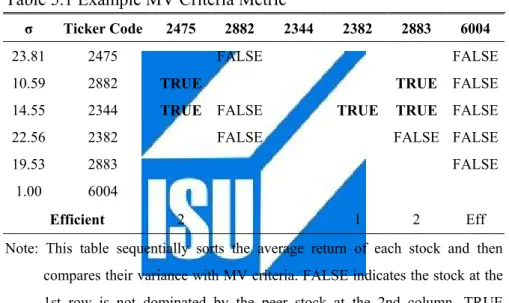
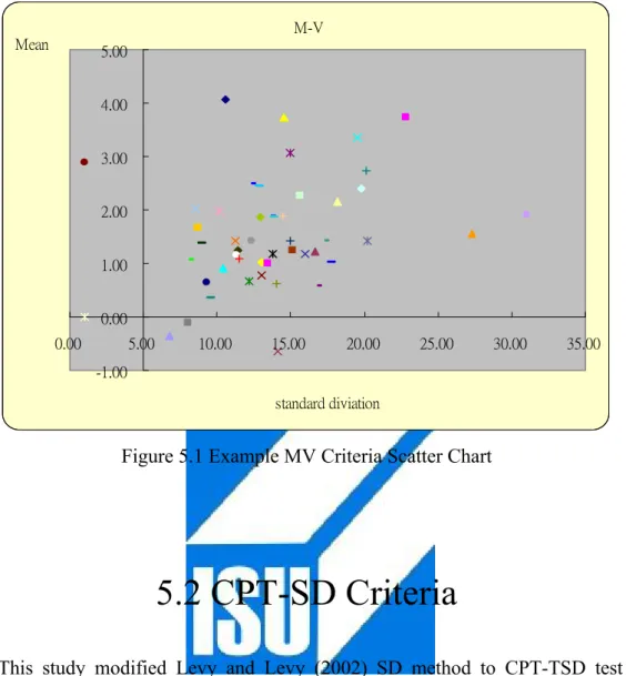
(37) Table 5.1 shows an MV criteria metric example of ETF 50 components sample filtered in March 2004. Subject to the same mean level, Stock“6505＂(Ticker Code) is not dominated by any other stocks because it has the lowest standard deviation. The example figure involved 50 sample stocks is also shown as Figure 5.1. We use the MV criteria metric to sort out MV candidate stocks in ETF 50 components in empirical study.. Table 5.1 Example MV Criteria Metric σ. Ticker Code. 23.81. 2475. 10.59. 2882. TRUE. 14.55. 2344. TRUE. 22.56. 2382. 19.53. 2883. 1.00. 6004 Efficient. 2475. 2882. 2344. 2382. 2883. FALSE FALSE. 6004 FALSE. TRUE. FALSE. TRUE. FALSE. TRUE. FALSE. FALSE FALSE FALSE. 2. 1. 2. Eff. Note: This table sequentially sorts the average return of each stock and then compares their variance with MV criteria. FALSE indicates the stock at the 1st row is not dominated by the peer stock at the 2nd column. TRUE indicates the stock at the 1st row is dominated by the peer stock at the 2nd column. Bland cell indicates even in pair-wise comparison.. 27.

(38) M-V Mean. 5.00 4.00 3.00 2.00 1.00 0.00 0.00. 5.00. 10.00. 15.00. 20.00. 25.00. 30.00. 35.00. -1.00 standard diviation. Figure 5.1 Example MV Criteria Scatter Chart. 5.2 CPT-SD Criteria This study modified Levy and Levy (2002) SD method to CPT-TSD test for determination if the difference the cumulative density functions of the returns of pair-wise ETF 50 component stocks are statistically significant. Because CPT predicts that people will choose prospects according to the value given by n. n. n. i =1. i =1. i =1. VF = VF+ + VF− = ∑ π i+ v( xi ) + ∑ π i− v( xi ) = ∑ π i v( xi ) π is decision weights that are calculated based on the “cumulative” probabilities associated with the outcomes.. 28.

(39) ,x≥0 ⎧ xα v( x) = ⎨ β ⎩ −λ ( − x ) , x < 0. α = 0.88, ß = 0.88, λ = 2.25 and. w− ( p ) =. pδ ( pδ + (1 − p)δ ). 1. w+ ( p ) =. δ. pγ ( pγ + (1 − p)γ ). 1. γ. δ =0.69, γ =0.61 Based on SD theorem, if stock Xi dominate stock Xj with CPT-SD, the cumulative leftmost distribution of Xi must nowhere exceed and at lest one point be strictly less than the cumulative rightmost distribution of Xj. In a first step, we set up. ( ) the Return Interval (R.I.) and then subjective value υ xi associated with each outcome is calculated. Next, we find out Return Probability (R.P.) and its cumulative return probability. Then the original cumulative probability is transformed with weighting function. Calculation details are enclosed by steps as follows. (1). Return Interval (R.I.) R.I. = Max (Return)-Min (Return)/T, T is here given to 50. (2). Value Transformation Separate profit and loss areas account for reference point and then intact value function to define positive prospect and loss prospect domains. (3). Return Probability (R.P.). 29.

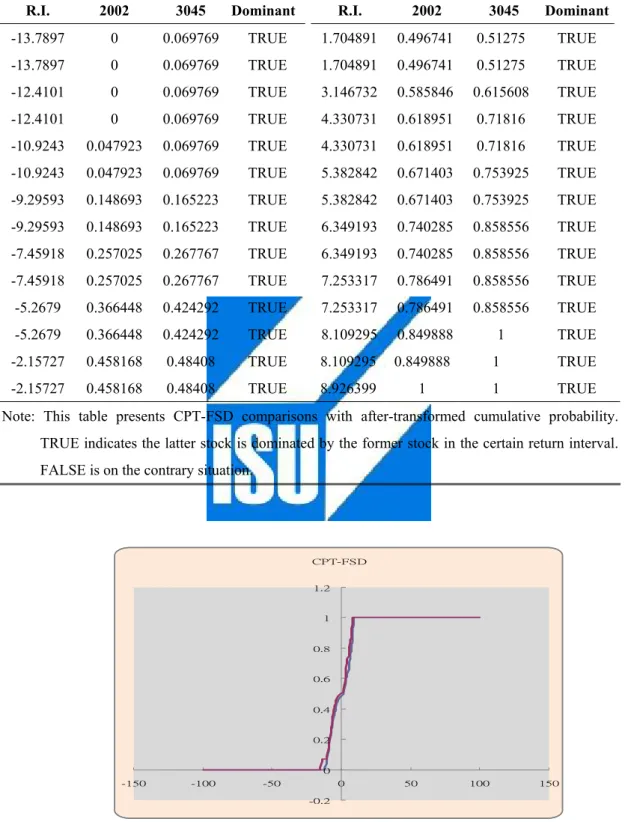
(40) Sum up the numbers of in each Return Interval and divided by total numbers to be specific return probability respectively. R.P. = Nj/NTotal (4). Calculate the Cumulative Return Probability (5). Cumulative Weighting Transformation Transform the original cumulative probability with positive weighting function ( W ( p ) ) if it lies on positive prospect of value function. Otherwise, the negative +. weighting function ( W ( p ) ) is used. −. (6). CPT-SD Pair-wised Metrics Like MV, we construct CPT-SD pair-wised metrics to filter out candidate stocks. Because of the hierarchical trait of SD, CPT-FSD example and CPT-SSD example and CPT-TSD example are demonstrated sequentially below. Consider two stocks identified by stock “2002” (ticker code) and stock“ 3045” in Table 5.2. Table 5.2 illustrates that if there exists even a very small amount of probability that the smallest outcome value in the leftmost distribution of stock“ 2002 ” is less than the smallest outcome value in the rightmost distribution of stock“3045”, then stock “2002 ”cannot dominate stock “3045 ”. In CPT-FSD test, stock “2002” is proved to dominate stock “3045 ” among each return interval (R. I.) as marked “True” in the last column of Table 5.2.. 30.

(41) Table 5.2 Sample CPT-FSD Test R.I.. 2002. 3045. Dominant. R.I.. 2002. 3045. Dominant. -13.7897. 0. 0.069769. TRUE. 1.704891. 0.496741. 0.51275. TRUE. -13.7897. 0. 0.069769. TRUE. 1.704891. 0.496741. 0.51275. TRUE. -12.4101. 0. 0.069769. TRUE. 3.146732. 0.585846. 0.615608. TRUE. -12.4101. 0. 0.069769. TRUE. 4.330731. 0.618951. 0.71816. TRUE. -10.9243. 0.047923. 0.069769. TRUE. 4.330731. 0.618951. 0.71816. TRUE. -10.9243. 0.047923. 0.069769. TRUE. 5.382842. 0.671403. 0.753925. TRUE. -9.29593. 0.148693. 0.165223. TRUE. 5.382842. 0.671403. 0.753925. TRUE. -9.29593. 0.148693. 0.165223. TRUE. 6.349193. 0.740285. 0.858556. TRUE. -7.45918. 0.257025. 0.267767. TRUE. 6.349193. 0.740285. 0.858556. TRUE. -7.45918. 0.257025. 0.267767. TRUE. 7.253317. 0.786491. 0.858556. TRUE. -5.2679. 0.366448. 0.424292. TRUE. 7.253317. 0.786491. 0.858556. TRUE. -5.2679. 0.366448. 0.424292. TRUE. 8.109295. 0.849888. 1. TRUE. -2.15727. 0.458168. 0.48408. TRUE. 8.109295. 0.849888. 1. TRUE. -2.15727. 0.458168. 0.48408. TRUE. 8.926399. 1. 1. TRUE. Note: This table presents CPT-FSD comparisons with after-transformed cumulative probability. TRUE indicates the latter stock is dominated by the former stock in the certain return interval. FALSE is on the contrary situation.. CPT-FSD 1.2. 1. 0.8. 0.6. 0.4. 0.2. 0 -150. -100. -50. 0. 50. -0.2. Figure 5.2 CPT-FSD Dominant. 31. 100. 150.

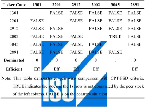
(42) Pair-wise dominance results for more stocks extended in Table 5.2 are shown in a matrix format in Table 5.3. An empty cell in the table indicates that no dominance could be established. There are 5 of 6 stocks are efficient or dominant candidate. It also shows the fact that CPT-FSD is not discriminated to each other.. Table 5.3 Sample CPT-FSD Metric Test Ticker Code. 1301. 1301. 2201. 2912. 2002. 3045. 2891. FALSE. FALSE. FALSE. FALSE. FALSE. FALSE. FALSE. FALSE. FALSE. FALSE. FALSE. FALSE. TRUE. FALSE. 2201. FALSE. 2912. FALSE. FALSE. 2002. FALSE. FALSE. FALSE. 3045. FALSE. FALSE. FALSE. FALSE. 2891. FALSE. FALSE. FALSE. FALSE. FALSE. Dominated. 0. 0. 0. 0. 1. Efficient. Eff. Eff. Eff. Eff. FALSE 0 Eff. Note: This table demonstrates pair-wise comparison with CPT-FSD criteria. TRUE indicates the stock at the 1st row is not dominated by the peer stock of the left column. FALSE is on the contrary situation.. Sample CPT-SSD calculations for stock “6505” and stock“2887” is shown in Table 5.4. Comparing CPT-FSD, we notice that stock “6505” and stock“2887” can be identified for dominant candidate in CPT-SSD test. In Figure 5.3, the cumulative distribution corresponding to stock “6505”does remain far below and to the right of the distribution corresponding to stock“2887”. Thus stock “6505” obviously dominates stock“2887” in CPT-SSD status.. 32.

(43) Table 5.4 CPT-SSD R.I.. 6505. 2887. Dominant. R.I.. 6505. 2887. Dominant. -13.7897. 0. 0.048476. TRUE. 3.146732. 1.01275. 2.067164. TRUE. -13.7897. 0. 0.048476. TRUE. 3.146732. 1.01275. 2.067164. TRUE. -12.4101. 0. 0.048476. TRUE. 4.330731. 1.01275. 2.552462. TRUE. -12.4101. 0. 0.048476. TRUE. 4.330731. 1.01275. 2.552462. TRUE. -10.9243. 0. 0.288794. TRUE. 5.382842. 1.01275. 3.104552. TRUE. -10.9243. 0. 0.288794. TRUE. 5.382842. 1.01275. 3.104552. TRUE. -9.29593. 0. 0.288794. TRUE. 6.349193. 1.01275. 3.730133. TRUE. -9.29593. 0. 0.288794. TRUE. 6.349193. 1.01275. 3.730133. TRUE. -7.45918. 0. 0.686055. TRUE. 7.253317. 1.01275. 4.459528. TRUE. -7.45918. 0. 0.686055. TRUE. 7.253317. 1.01275. 4.459528. TRUE. -5.2679. 0. 0.941872. TRUE. 8.109295. 1.01275. 5.367062. TRUE. -5.2679. 0. 0.941872. TRUE. 8.109295. 1.01275. 5.367062. TRUE. -2.15727. 0. 1.242188. TRUE. 8.926399. 1.01275. 5.367062. TRUE. -2.15727. 0. 1.242188. TRUE. 8.926399. 1.01275. 5.367062. TRUE. 1.704891. 0.256375. 1.614758. TRUE. 9.711153. 1.01275. 5.367062. TRUE. 1.704891. 0.256375. 1.614758. TRUE. 9.711153. 1.01275. 5.367062. TRUE. Note: This table presents CPT-SSD comparisons with after-transformed cumulative probability. TRUE indicates the latter stock is dominated by the former stock in the certain return interval. FALSE is on the contrary situation.. CPT-SSD. 6. 5. 4. 3. 2. 1. 0 -150. -100. -50. 0. 50. -1. Figure 5.3 CPT-SSD Dominant. 33. 100. 150.

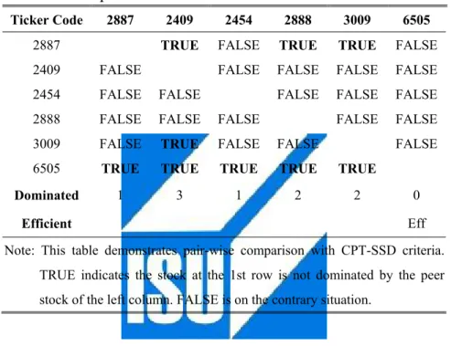
(44) Example pair-wise dominance results for more stocks extended in Table 5.4 are also cross tested in Table 5.5. There is only 1(stock “6505”) of 6 stocks to be identified efficient or dominant candidate. It shows the advantage that CPT-SSD is more discriminated to CPT-FSD.. Table 5.5 Sample CPT-SSD Metric Test Ticker Code. 2887. 2887. 2409. 2454. 2888. 3009. 6505. TRUE. FALSE. TRUE. TRUE. FALSE. FALSE. FALSE. FALSE. FALSE. FALSE. FALSE. FALSE. FALSE. FALSE. 2409. FALSE. 2454. FALSE. FALSE. 2888. FALSE. FALSE. FALSE. 3009. FALSE. TRUE. FALSE. FALSE. 6505. TRUE. TRUE. TRUE. TRUE. TRUE. Dominated. 1. 3. 1. 2. 2. FALSE. 0 Eff. Efficient. Note: This table demonstrates pair-wise comparison with CPT-SSD criteria. TRUE indicates the stock at the 1st row is not dominated by the peer stock of the left column. FALSE is on the contrary situation.. To integrate TSD into CPT, we let F and G be the cumulative distribution functions (CDFs) and f and g are their probability density functions (PDFs) of the S shape prospects for two stocks A and B respectively. Define 3 H0 =h and H3(x) =∫. r. a. H2 (t) dt for h=f, g and H=F, G. Stock A would dominate Stock B by CPT-TSD. if and only if AF3(x) ≤ BG3(x) for all x, and the strict inequality holds for at least one value of x; and A has higher expected return distribution than B. The existence of CPT-TSD implies that the expected utilities of investors are comparatively higher. 3. Refer to Anderson (2004) and Wong et al. (2008) for the detail discussions on the definitions. 34.

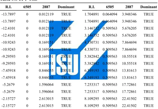
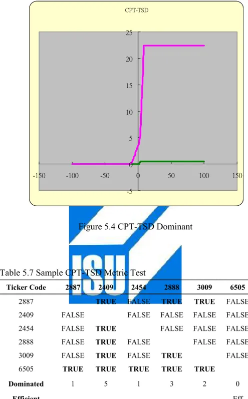
(45) when holding the dominant stock than the dominated stock, and surely the dominated stock will not be selected in CPT-TSD portfolio. In Table 5.6, stock “6505” dominates stock “2887” through different R.I. and Figs. 5.4 illustrate CPT-TSD tests graphically. Table 5.7 shows stock “6505” still dominate, already dominant in CPT-SSD, the other stocks in the strictest dominated requirement.. Table 5.6 CPT-TSD R.I.. 6505. 2887. Dominant. -13.7897. 0. 0.012119. TRUE. -13.7897. 0. 0.012119. -12.4101. 0. -12.4101. R.I.. 6505. 2887. Dominant. 1.704891 0.064094. 3.948346. TRUE. TRUE. 1.704891 0.064094. 3.948346. TRUE. 0.012119. TRUE. 3.146732 0.509563. 5.676205. TRUE. 0. 0.012119. TRUE. 3.146732 0.509563. 5.676205. TRUE. -10.9243. 0. 0.169151. TRUE. 4.330731 0.509563. 7.864694. TRUE. -10.9243. 0. 0.169151. TRUE. 4.330731 0.509563. 7.864694. TRUE. -9.29593. 0. 0.169151. TRUE. 5.382842 0.509563. 10.55518. TRUE. -9.29593. 0. 0.169151. TRUE. 5.382842 0.509563. 10.55518. TRUE. -7.45918. 0. 0.846055. TRUE. 6.349193 0.509563. 13.81613. TRUE. -7.45918. 0. 0.846055. TRUE. 6.349193 0.509563. 13.81613. TRUE. -5.2679. 0. 1.596064. TRUE. 7.253317 0.509563. 17.72861. TRUE. -5.2679. 0. 1.596064. TRUE. 7.253317 0.509563. 17.72861. TRUE. -2.15727. 0. 2.613015. TRUE. 8.109295 0.509563. 22.41502. TRUE. -2.15727. 0. 2.613015. TRUE. 8.109295 0.509563. 22.41502. TRUE. Note: This table presents CPT-TSD comparisons with after-transformed cumulative probability. TRUE indicates the latter stock is dominated by the former stock in the certain return interval. FALSE is on the contrary situation.. 35.

(46) CPT-TSD. 25. 20. 15. 10. 5. 0 -150. -100. -50. 0. 50. 100. 150. -5. Figure 5.4 CPT-TSD Dominant. Table 5.7 Sample CPT-TSD Metric Test Ticker Code. 2887. 2887. 2409. 2454. 2888. 3009. 6505. TRUE. FALSE. TRUE. TRUE. FALSE. FALSE. FALSE. FALSE. FALSE. FALSE. FALSE. FALSE. FALSE. FALSE. 2409. FALSE. 2454. FALSE. TRUE. 2888. FALSE. TRUE. FALSE. 3009. FALSE. TRUE. FALSE. TRUE. 6505. TRUE. TRUE. TRUE. TRUE. TRUE. Dominated. 1. 5. 1. 3. 2. FALSE. 0 Eff. Efficient. Note: This table demonstrates pair-wise comparison with CPT-TSD criteria. TRUE indicates the stock at the 1st row is not dominated by the peer stock of the left column. FALSE is on the contrary situation.. 36.

(47) In Taiwan, The first and most popular ETF product, TWSE Taiwan 50 Index (Ticker Code 0050), was launched on October 29, 2002. The first tradable index for the Taiwan market was created under the collaboration of Taiwan Stock Exchange Corporation ("TWSE") and FTSE International Limited ("FTSE"). This Index covers the top 50 companies by total market capitalization. The source of the data for this study is Taiwan Economic Journal Database (TEJ), the pre-eminent information repository of Taiwan stock market data. Monthly and weekly total return data for ETF50 Components was compiled beginning with observations for 1998 and ending with 2008. The sample period 1998 through 2008 wholly incorporates our database. Each rate of return observation measures a particular stock's net monthly and weekly performance. The 50 historical data of component stocks in continuous existence between 1998 and 2002 comprise the first population for data integrity. The terminal value of benchmark ETF50 is measure with TWSE Taiwan50 Index-Total Return Index for correction of dividend issuance. We sort stocks from ETF 50 by four different portfolio strategies to set up the fundamental investment group. Meanwhile, the monthly return sorting and weekly returns sorting groups are separated for research discussion. It is worthy to note that each strategy infuses revised portfolios which are crafted from changes in the composition of the efficient set of stocks induced by subsequent month/week of rates of return data. Thus portfolios are refreshed rather than unchanged in this strategy. The portfolio is then revised as a consequence of and in reaction to the new set of efficient funds deduced by stochastic dominance analysis for the period 2003-2008. Twenty four portfolios in the 2003-2008 efficient set quarterly retain their status.. 37.

(48) We also allocate different weighting to each selected stocks by four different tactics. They are equal-weighted method, price-weighted method, random-weighted method and volume-weighted method. Equal weighted tactics is defined as the average allocation of money in candidate stocks. The percentage of price weighted tactics depends on the market value of the candidate stock in the portfolio. The random weighted allocation is a special trick we use here to conjecture investor’s discretion. We let the allocated percentage of those sorted stocks be randomly assigned. To consider quantity factor, the allocation percentage by volume weighted method is judged by its turnover in all of the sorting stocks. That design is to find which tactics is the best in all strategies and which strategy is the best in all tactics and the fitness between them as well. The summarized research design of this study is shown in Figure 5.5. For examine sensitivity to time horizon of our findings. We split three time horizon, 1 year, 3 year and 5 year and total time level( year 2003-2008), for different upward (bull market) and downward market (bear market) situation. This is to find the performance difference in opposite market direction movement and consider the robustness of performance persistence. In addition to total return performance comparison, the ranking priority test is employed into 16 panels on the basis of four strategies and four tactics as the paper structured. Lastly, we check if the CPT-TSD strategy evidently downsizes original portfolio (ETF 50) numbers. To call on the CPT-TSD strategy application, our purpose of this. 38.

(49) study, the construction contents of MV and CPT-TSD portfolios are both compared insightfully from their reinvestment traits and between-group difference.. 39.

(50) ETF 50. M-V. Frontier (Monthly/Weekly). Equal Weighted. Total Return Comparisons. CPT-FSD. CPT-SSD. Dominant (Monthly/Weekly). Dominant (Monthly/Weekly). Price Weighted. Return Ranking. CPT-TSD. Dominant (Monthly/Weekly). Random Weighted. Volume Weighted. Portfolio Difference. Portfolio Repetition. N=N+1. No. Last. Figure 5.5 Research Design. 40. Yes. Stop.

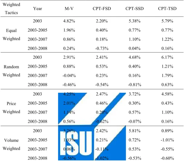
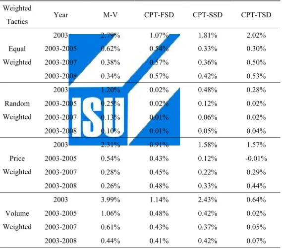
(51) 6. Empirical Results 6.1 Performance of Portfolios Sorted by Monthly Return The first application of four different strategies considers the 1 year, 3 years, 5 years and total time frame. A collective summary of the empirical findings of these strategies appears in Table 6.1. Portfolio performance Screened by Cumulative Prospect Theory-First Degree Stochastic Dominance (CPT-FSD) is clearly inferior on the monthly return sorted basis no matter which tactics is considered. In year 2003, it earned only almost 2.20% to 2.40% in each weighted tactics, less than MV’s 2.91% to 4.82%. The more restrictive Cumulative Prospect Theory-Second Degree Stochastic Dominance (CPT-SSD) criterion performed better especially considering volume weighted tactics. Opposite to CPT-FSD, The Cumulative Prospect Theory-Third Degree Stochastic Dominance (CPT-TSD) had outstanding performance in year 2003. A surprising result is that CPT-TSD was poor matched with volume weighted allocation.. 41.

(52) Table 6.1 Performance of Portfolios Sorted by Monthly Return in Different Strategies, 2003-2008 Weighted. Year. M-V. CPT-FSD. CPT-SSD. CPT-TSD. 2003. 4.82%. 2.20%. 5.38%. 5.79%. Equal. 2003-2005. 1.96%. 0.40%. 0.77%. 0.77%. Weighted. 2003-2007. 0.86%. 0.18%. 1.10%. 1.22%. 2003-2008. 0.24%. -0.73%. 0.04%. 0.16%. 2003. 2.91%. 2.41%. 4.68%. 6.17%. Random. 2003-2005. 0.88%. 0.53%. 0.40%. 1.21%. Weighted. 2003-2007. -0.04%. 0.23%. 0.16%. 1.79%. 2003-2008. -0.46%. -0.54%. -0.81%. 0.63%. 2003. 4.25%. 2.47%. 3.72%. 4.58%. Price. 2003-2005. 2.01%. 0.46%. 0.30%. 0.43%. Weighted. 2003-2007. 1.14%. 0.20%. 0.57%. 1.10%. 2003-2008. 0.56%. -0.62%. -0.07%. 0.16%. 2003. 3.26%. 2.42%. 5.81%. 0.89%. Volume. 2003-2005. 1.03%. 0.21%. 0.72%. -1.01%. Weighted. 2003-2007. 0.06%. -0.11%. 0.53%. -0.55%. 2003-2008. -0.56%. -1.02%. -0.53%. -0.60%. Tactics. Notes: This table reports performance of MV, CPT-FSD, CPT-SSD, CPT-TSD portfolios, sorted by monthly return, in four weighted tactics.. 6.2 Performance of Portfolios Sorted by Weekly Return On the basis of weekly return sorted, we obtained in some extent different to the performance of monthly return sorted. In general, MV strategy has superior returns across strategy classification and tactics consideration. Contrarily, it is obviously disadvantaged to use CPT-SD strategy on the basis of weekly return sorted. Even though the unique performance of MV portfolio on the weekly return sorted basis, it is 42.