以資料為中心之類神經網路方法論與離群值

行政院國家科學委員會專題研究計畫 成果報告

以資料為中心之類神經網路方法論與離群值

研究成果報告(精簡版)

中 華 民 國 101 年 07 月 31 日

中 文 摘 要 ： 當我們進行資料探勘應用，需要考慮到離群值的影響。然 而，有效地識別離群值仍然是一個研究的議題。本研究借由 修改 Tsaih & Cheng（2009）的穩健學習演算法（resistant learning algorithm），研提出信封程序法（envelope procedure），以有效地識別離群值。本研究設計了一個 100 次模擬運行之實驗；每次模擬運行各自有不同的 100 個觀測 數據集。此實驗乃用來展示研提的信封程序法之運算過程以 及其識別離群值的表現；其實驗結果是相當正面的。 中文關鍵詞： 穩健學習情境、離群值、單一隱藏層倒傳遞神經網路、前進 選擇法

英 文 摘 要 ： When we conduct the data mining application, the outlier issue needs to be taken into consideration. However, it is still a study issue to effectively identify the outlier in the context of resistant learning, where the fitting function form is unknown and outliers are the observations far away from the fitting function deduced from the majority of given observations. In contrast with the resistant learning algorithm proposed by Tsaih & Cheng (2009) that uses a tiny ε value, this study proposes the envelope procedure with a non-tiny ε value that results in a nonlinear fitting function f around with the envelope whose width being equal to 2ε. The envelope should contain at least n observations at the nth stage. This is distinct to the idea of Tsaih & Cheng (2009) that wants to evolve the fitting function to almost precisely fit all of n reference observations at the nth stage (because that the corresponding  value is tiny). Furthermore, the proposed envelope procedure should help identify the outlier via less computation than the resistant learning algorithm of Tsaih & Cheng (2009). An experiment with 100 simulation runs, each of which has a different set of 100 observation data, is conducted to demonstrate the proposed

envelope procedure and its performance of identifying the outliers. And the experimental result is

positive.

英文關鍵詞： resistant learning； outliers； single-hidden layer feed-forward neural networks； forward selection

摘要 

當我們進行資料探勘應用，需要考慮到離群值的影響。然而，有效地識別離群值

仍然是一個研究的議題。本研究借由修改Tsaih & Cheng（2009）的穩健學習演

算法（resistant learning algorithm），研提出信封程序法（envelope procedure），以

有效地識別離群值。本研究設計了一個100 次模擬運行之實驗；每次模擬運行各 自有不同的100 個觀測數據集。此實驗乃用來展示研提的信封程序法之運算過程 以及其識別離群值的表現；其實驗結果是相當正面的。 關鍵詞：穩健學習情境、離群值、單一隱藏層倒傳遞神經網路、前進選擇法 ABSTRACT

When we conduct the data mining application, the outlier issue needs to be taken into consideration. However, it is still a study issue to effectively identify the outlier in the context of resistant learning, where the fitting function form is unknown and outliers are the observations far away from the fitting function deduced from the majority of given observations. In contrast with the resistant learning algorithm proposed by Tsaih & Cheng (2009) that uses a tiny ε value, this study proposes the envelope procedure with a non-tiny ε value that results in a nonlinear fitting function f around with the envelope whose width being equal to 2ε. The envelope should contain at least n observations at the nth stage. This is distinct to the idea of Tsaih & Cheng (2009) that

wants to evolve the fitting function to almost precisely fit all of n reference observations at the nth _{stage (because that the corresponding  value is tiny).}

Furthermore, the proposed envelope procedure should help identify the outlier via less computation than the resistant learning algorithm of Tsaih & Cheng (2009). An

experiment with 100 simulation runs, each of which has a different set of 100 observation data, is conducted to demonstrate the proposed envelope procedure and its performance of identifying the outliers. And the experimental result is positive.

Keywords: resistant learning; outliers; single-hidden layer feed-forward neural networks; forward selection

1. The introduction

In modern financial markets whose input-output relationship is believed to be non-linear yet unknown, there are occasionally outliers that are far from the bulk of vast amounts of observations. Outliers are rare events since the sample size of the outlier compared with the normal majority is relatively low. The unidentified outliers can deteriorate the result of the data mining application. However, to effectively identify the outlier is still a study issue. For instance, Agyemang et al. (2006) point out that outlier detection is a very complex task akin to find a needle in a haystack. Similarly, Ngai et al. (2010) summarize that, in the case of financial fraud detection, the detection of the fraud case may be regarded as recognizing the outlier from the healthy majority and the data mining techniques of outlier detection has seen only limited use. The outlier study is in the context of robust nonlinear modeling or

resistant learning without knowing the fitting function form.

In the context of estimating, the response y is modeled as f(x, w) +  where w is the parameter vector and  is the error term. The function form of the fitting function f is predetermined and fixed during the process of deriving its associated w from a set of given observations {(x1, y1), …, (xN, yN)}, with yc being the observed response

corresponding to the cth observation xc. The least squares estimator (LSE) is one of the most popular methods for the estimating. If wˆ denotes any estimate of w, then LSE is defined to the wˆ that minimizes N

c 1(e

c₎2_{, in which}

ec = yc - f(xc, w). (1)

The generalized delta rule proposed by Rumelhart et al. (1986) is a kind of nonlinear LSE. The LSE, however, is known to be very sensitive to outliers, the observations that are far away from the deduced fitting function f.

In the context of resistant learning, the function form of f is adaptable during the process of deducing its associated w from a set of given observations {(x1, y1), …, (xN,

yN)}. Here “resistant” is equivalent to “robust.” The terms “robust” and “resistant” are often used interchangeably in the statistical literature, but sometimes have specific meanings (Huber 1981, page 4). Robust procedures are those whose results are not impacted significantly by violations of model assumptions. Resistant procedures are those whose numerical results are not impacted significantly by outlying observations. Windham (1995) proposes a procedure to robustify any model fitting process by

using weights from a parametric family from which the model is to be chosen, and refers it as “robust model fitting.” Methods for model selection and/or variable selection in the presence of outliers have been discussed in (Hoeting et al. 1996; Atkinson and Riani 2002). Knorr and Ng (1997)(1998)(2000) focus on the development of algorithms for identifying the distance-based outliers in large data sets. All these methods are based on a family of parametric models or a given model form with several independent variables. These works do not seem to generalize to the resistant learning problems studied here.

Tsaih & Cheng (2009) proposed the resistant learning algorithm with a tiny pre-specified ε value (say 10-6_{) that can deduce proper nonlinear function form f}

and

wˆ such that |yc - f(xc,wˆ)|  ε for all c. The resistant learning algorithm essentially

adopts both robustness analysis and deletion diagnostics to cope with the presence of outliers. The robustness analysis entails adopting the idea of C-step for deriving an (initial) subset of m+1 reference observations to fit the linear regression model, ordering the residuals of all N observations at each stage, and then augmenting the reference subset gradually based upon the smallest trimmed sum of squared residuals principle. At the same time, the weight-tuning mechanism, the recruiting mechanism, and the reasoning mechanism allow the SLFN to adapt dynamically during the process and to be able to explore an acceptable nonlinear relationship between

explanatory variables and the response in the presence of outliers. The deletion diagnostic approach is employed with the proposed diagnostic quantity as the number of pruned hidden nodes when one observation is excluded from the reference pool. This diagnostic quantity indicates whether the SLFN is stable. However, the computation of such a deletion diagnostic mechanism is rather complicated and time-consuming when the size of the reference pool is large.

In contrast with the resistant learning algorithm proposed by Tsaih & Cheng (2009) that uses a tiny ε value, this study proposes the envelope procedure with a non-tiny ε value that results in a nonlinear fitting function f around with the envelope whose width being equal to 2ε. The envelope should contain at least n observations at the nth stage. This is distinct to the idea of Tsaih & Cheng (2009) that wants to evolve the fitting function to almost precisely fit all of n reference observations at the nth stage (because that the corresponding  value is tiny). Furthermore, the proposed envelope procedure should help identify the outlier via less computation than the resistant learning algorithm of Tsaih & Cheng (2009).

The setting of the ε value is dependent on the user’s perception about the data and the associated outliers. For instance, if the perceptions are that the error is normally distributed, with mean 0 and variance 1, and the outliers are the ones with residuals greater than 1.96 in absolute value. These perceptions are similar to the setting in the regression analysis corresponding to 5% of significance level given the normal distribution. Then, the user can set the  value of the proposed envelope procedure as 1.96, the threshold for the outlier.

In short, here the identified outlier is data-based. Namely, the fitting function f is deduced from the current reference observations at each stage and the outliers are the ones whose deviation from the deduced fitting function f are greater than 2.5 times of the standard deviation of the residuals of the current reference observations. According to the 3-sigma rule, about 98.7% of the observations lie within 2.5 standard deviations away from the mean; therefore, 1.3% of the observations are identified as the outlier.

Here we use single-hidden layer feed-forward neural networks (SLFN) to illustrate the proposed envelope procedure, where the number of adopted hidden nodes of SLFN is adaptable and potential outliers should not impact significantly the number of adopted hidden nodes at the early stages of process.

The rest of this paper is organized as follows: the proposed envelope procedure and its justification are introduced in Section 2. An illustrative experiment is presented in Section 3. Finally, conclusions and future research directions are presented.

2. The proposed envelope procedure

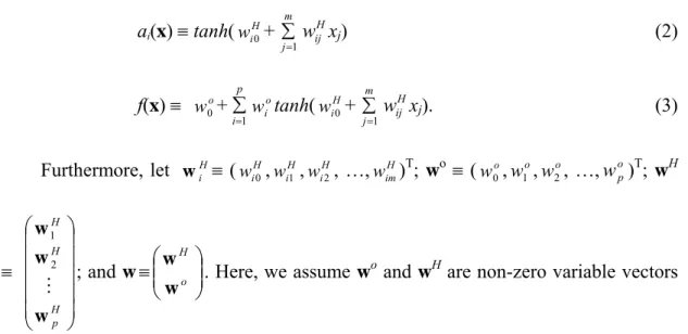
The SLFN is defined in equations (2) and (3), where tanh(x)  _xx _xx e e e e     ; m is the number of explanatory variables xj’s; p is the number of adopted hidden nodes;

H i

w₀ is the bias value of the ith hidden node; the superscript H throughout the paper refers to quantities related to the hidden layer; H

ij

w is the weight between the jth

explanatory variable xj and the ith hidden node; w₀o is the bias value; the superscript o throughout the paper refers to quantities related to the output layer; and o _{is the}

weight between the ith hidden node and the output node. In this article, a character in bold represents a column vector, a matrix, or a set, and the superscript T indicates the transposition. ai(x)  tanh(wiH0+ m j 1  H ij w xj) (2) f(x)  _wo 0+ p i 1 o i w tanh( H i w0+ m j 1  H ij w xj). (3) Furthermore, let H i w  (w_iH₀,w_iH₁,w_iH₂, …,w_imH)T; wo  (w₀o,w₁o,w₂o, …,w )o_p T; wH                H p H H w w w  2 1 ; and w _      o H w w

. Here, we assume wo and wH are non-zero variable vectors

and p is an integer variable that is always positive. Note that, since the value of p is adjustable, the (nonlinear) function form of f is adaptable and the hyperbolic tangent function is used here as the base of f.

Through this SLFN, the input information x is first transformed into a  (a1,

a2, …, ap)T, and the corresponding value of f is generated by a rather than x. That is, given the observation x, all corresponding values of hidden nodes are first calculated with a_i= tanh( H i w0 + m j 1  H ij

w x_j ) all i and the corresponding value f(x) is then

calculated as f(x) = g(a)  _wo 0+ p i 1  o i w ai.

Table 1 presents the proposed envelope procedure. Assume that there is a total of N observations, N  m+1, and xi _{ x}j _{when i  j. Let I(N) be the set of indices of all} observations. Let the nth stage of the corresponding process, N  n > m+1, be the stage of handling n reference observations which are the ones with the smallest n squared residuals among N squared residuals, and I(n) be the set of indices of these reference

observations. At the nth stage, we look for an acceptable SLFN estimate that leads to a set of {(xc, yc): c  Iˆ n( )} with (ec)2  ε2 for all c  ˆ nI( ) and I(n)  Iˆ n( ), where ec

is defined in equation (1) and 2ε is equal to the pre-specified width of the envelope. In other words, at the end of the nth stage, the acceptable SLFN estimate presents a fitting function f around with an envelope that contains at least these n observations {(xc, yc): c  Iˆ n( )}. Let I(n) be the set of indices of (xc, yc) with the smallest n squared residuals among N squared residuals at the end of the nth _stage. I(n) may not be equal to I(n).

Table 1: The proposed envelope procedure.

Step 1: Arbitrarily obtain the initial m+1 reference observations. Let I(m+1) be the set of indices of these observations. Set up an acceptable SLFN estimate with one hidden node regarding the reference observations {(xc, yc): c  I(m+1)}. Set n = m+2.

Step 2: If n > N, STOP.

Step 3: Present the n reference observations (xc, yc) that are the ones with the smallest n squared residuals among current N squared residuals. Let I(n) be the set of indices of these observations.

Step 4: If ₂ 2 2 2 ) 1 ( ) 1 ( ) (    N n ec  _{ c  I(n), go to Step 7.}

Step 5: Assume   I(n), ₂

2 2 2 ) 1 ( ) 1 ( ) (    N n e  , and ₂ 2 2 2 ) 1 ( ) 1 ( ) (    N n ec  _{ c } I(n)-{}. Set w~ = w.

Step 6: Apply the gradient descent mechanism to adjust weights w until one of the following two cases occurs:

(1) If the deduced envelope contains at least n observations, go to Step 7.

(2) If the deduced envelope does not contain at least n observations, then set w = w~ and apply the augmenting mechanism to add extra hidden nodes to

obtain an acceptable SLFN estimate.

Step 7: Implement the pruning mechanism to delete all potentially irrelevant hidden nodes; n + 1  n; go to Step 2. 

The proposed envelope procedure in Table 1 consists of the following two sub-procedures: (i) the ordering sub-procedure implemented in Step 3 that determines the input sequence of reference observations and (ii) the modeling sub-procedure implemented in Step 6 and Step 7 that adjusts the number of hidden nodes adopted in the SLFN estimate and the associated w to evolve the fitting function f and its envelope to contain at least n observations. The details are explained as follows.

In Step 1, we arbitrarily obtain the initial m+1 reference observations {(xc, yc): c  I(m+1)}. The number m+1 is also equal to the number of the associated H

1

w and

H

w₁₀. We use the data set {(xc, tanh-1(

2 min max 1 min ) ( ) ( ) (        c N c c N c c N c c y y y y I I

I )): c  I(m+1)} to set up the

system (4), which is a system of m+1 linear equations in m+1 unknowns. Then, the values of _wo

0 and

o

w1 are assigned as min 1

)

( 



c N

cI y and max( )  min( ) 2

c N c c N c I y I y

respectively. Step 1 uses the weight values _wH

10 and

H

1

w obtained from solving the

system (4) and the assigned values of _wo

0 and

o

w1 to set up an acceptable SLFN estimate that renders (ec)2 = 0  2 2₂

) 1 (N m  ₌ 2 2 2 ) 1 ( ) 1 1 (    N m  _{,  c  I(m+1).} H w10+ m j 1  H j w₁ c j x = tanh-1( 2 min max 1 min ) ( ) ( ) (        c N c c N c c N c c y y y y I I I ₎  c  I(m+1). ₍₄₎

At the nth stage, Step 3 presents the n reference observations {(xc, yc): c  I(n)}

that are the ones with the smallest n squared residuals among current N squared residuals and are used to evolve the fitting function. The concept of forward selection (Atkinson and Cheng 1999) is adopted in Step 3 – the ordering of residuals of all N reference observations is used to determine the input sequence of reference

observations.  However, I(n) may not equal I(n). Namely, some of the reference observations at the early stages might not stick in the set of reference observations at the later stages, although most of them will.

Note that, at the end of the n-1th _{stage, {(x}c_{, y}c_{): c  (n1)}

I } are the ones with

the smallest n-1 squared residuals among N squared residuals and ₂

2 2 2 ) 1 ( ) 2 ( ) (    N n ec 

 c  I(n1). Thus, at Step 3, {(xc, yc): c  I(n)} = {(xc, yc): c  I(n1)}  {(x,

y)}, where ₂ 2 2 2 ) 1 ( ) 1 ( ) (    N n ec  _{ c  (n1)}

I and (x, y) is the one with the nth

smallest squared residuals among current N squared residuals at the beginning of the nth stage. (x, y) is named as the next point at the nth stage. Therefore, at Step 4, to

check if ₂ 2 2 2 ) 1 ( ) 1 ( ) (    N n

ec  _{ c  I(n) is the same as to check if}

2 2 2 2 ) 1 ( ) 1 ( ) (    N n e  . If ₂ 2 2 2 ) 1 ( ) 1 ( ) (    N n e  , then ₂ 2 2 2 ) 1 ( ) 1 ( ) (    N n

ec  _{ c  I(n), there is only the pruning}

mechanism of Step 7 involved, and the next stage can proceed. If ₂

2 2 2 ) 1 ( ) 1 ( ) (    N n e  , we still have ₂ 2 2 2 ) 1 ( ) 1 ( ) (    N n ec  _{ c  I(n)-{}

} and Step 6 is executed.

The modeling sub-procedure implemented at Step 6 to Step 7 seeks proper values of w and p so that the deduced envelope contains at least n observations at the end of the nth stage. Specifically, at the beginning of Step 6, the gradient descent mechanism is applied to adjust weights w. One of the gradient descent mechanisms

proposed in the literature is the weight-tuning mechanism of Tsaih & Cheng (2009) for min (w) w En c I ((n) o w0+ p i 1  o i w tanh( H i w0+ m j 1  H ij w x ) - yc_j c)2 + 1||w||2. However, the

result of implementing the gradient descent mechanism may get stuck in a local optimum. Another possible scenario of getting stuck in a local optimum is when the SLFN estimate obtained at the previous stage is defective regarding the modeling job of the current stage, i.e., the current number of hidden nodes is not sufficient to render the SLFN estimate to work well for the modeling job of the current stage. Both scenarios lead to an unacceptable SLFN estimate regarding the reference observations, and unfortunately, at present there is no perfect optimization mechanism to simultaneously cope with both scenarios.

Step 6.2 restores the w~ that is stored in Step 5. Thus we return to the previous

SLFN estimate that renders ₂

2 2 2 ) 1 ( ) 1 ( ) (    N n e  and ₂ 2 2 2 ) 1 ( ) 1 ( ) (    N n ec  _{ c }

I(n)-{}. Then the augmenting mechanism should recruit extra hidden nodes to

render ₂ 2 2 2 ) 1 ( ) 1 ( ) (    N n

ec  _{ c  I(n). One of augmenting mechanisms proposed in}

the literature is the recruiting mechanism of Tsaih & Cheng (2009) that adds two extra

hidden nodes to the previous SLFN estimate to render ₂

2 2 2 ) 1 ( ) 1 ( ) (    N n ec  _{ c  I(n).}

To decrease the complexity (and thus to reduce the overfitting likelihood) of the fitting function f, the pruning mechanism is proposed in Step 7 to delete potentially irrelevant hidden nodes. At the nth stage, a hidden node is potentially irrelevant if it is deleted and the application of the gradient descent mechanism can accomplish the goal that the obtained envelope contains at least n observations. A defective SLFN estimate triggers the augmenting mechanism in Step 6.2, but the situation of leading

to an undesired local minimum also triggers the augmenting mechanism. Thus, the augmenting mechanism may recruit excess hidden nodes that later become irrelevant. The irrelevant hidden nodes are useless with respect to the learning goal, and they may result in the overfitting likelihood of the fitting function f. One of pruning mechanisms proposed in the literature is the reasoning mechanism of Tsaih & Cheng (2009).

Although Step 4 to Step 7 presented in this study is similar with the ones presented by Tsaih & Cheng (2009), the  value adopted here is much larger than the one in (Tsaih & Cheng 2009). Namely, the proposed envelope procedure wants to evolve the fitting function around with an envelope to contain at least n observations at the nth stage. This is distinct to the idea of Tsaih & Cheng (2009) that wants to evolve the fitting function to almost precisely fit all of the reference observations {(xc, yc_{): c  I(n)} at the n}th _{stage (because that the corresponding  value is tiny).}

Since we assume that the errors follow normal distribution N(0,2_{), at Step 3 of}

the nth stage, we will calculate the standard deviation of (ec)2 of {(xc, yc): c  )

1 (n

I } and the deviation of the next point (x, y) from the current fitting function f. If n  0.75N and the residual of the next point is greater than 2.5 times of the standard deviation of the residuals of the current reference observations, then the next point is recorded as the identified outlier. According to the 3-sigma rule, about 98.7% of the observations lie within 2.5 standard deviations away from the mean; therefore, 1.3% of the observations are identified as the outlier.

In short, the proposed envelope procedure is data-based. That is, at the nth stage, the envelope is evolved to contain the reference observations of {(xc, yc): c 

) 1 (n

deviation from the fitting function f is greater than 2.5 times of the standard deviation of the residuals of {(xc, yc): c  I(n1)}.

3. AN ILLUSTRATIVE EXPERIMENT

In this section, we present the simulation results for evaluating the proposed procedure. That is, we apply the proposed envelope procedure to 100 simulation runs to evaluate the effectiveness of detecting the theoretical outliers. For each simulation run, we use the nonlinear model stated in equation (7) to generate a set of 100 observations where the explanatory variable X is equally spaced from 0.0 to 20.0 and the error is normally distributed, with mean 0 and variance 1. Here the theoretical fitting function f is the one stated in equation (7) and the theoretical outliers are the ones with residuals regarding the equation (7) greater than 1.96 in absolute value. This definition is similar to the setting in the regression analysis corresponding to 5% of significance level given the normal distribution. Here, we set the  value of the proposed envelope procedure as 3 that is smaller but close to 1.96, the threshold for the theoretical outlier.

Y=0.5 + 0.4*X + 0.8*Exp(-X) + Error (7)

Table 2 shows the information of the number of the simulation runs regarding the number of theoretical outliers contained in each observation set. For instance, there are 16 simulation runs each of which has 3 theoretical outliers. On average there are 4.97 theoretical outliers in each observation set.

Table 2: The number of the simulation runs regarding the number of theoretical outliers contained in the observation set.

The number of associated

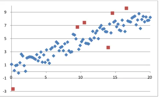
1 2 2 11 3 16 4 14 5 17 6 21 7 7 8 5 9 4 11 3 Without losing the generalization, the 10th observations set shown in Figure 1 is used to illustrate the effect of the proposed envelope procedure. Among 100 observations, there are six theoretical outliers marked as the square shown in Figure 1.

Figure 1: The plot of {(xc, yc)} of the 10th observation set.

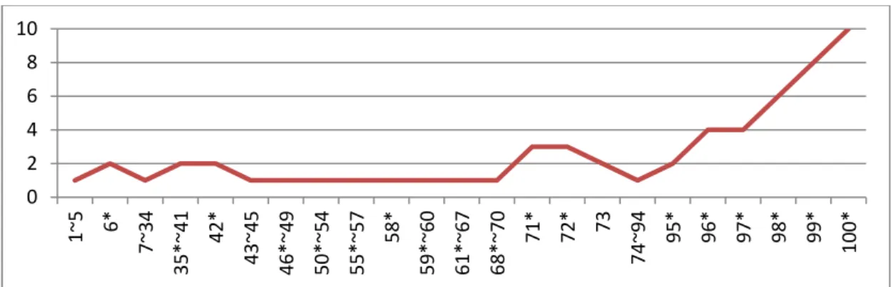
Figure 2 is the plot of the number of adopted hidden nodes at the end of each stage within the 10th simulation run. In Figure 2, for instance, 7 ~ 34 denotes that, from the 7th stage to the 34th stage, the criterion of Step 4 is satisfied and there is no adjustment of the fitting function f resulted from the pruning mechanism implemented at Step 7. Furthermore, the * sign denotes the stage where the criterion of Step 4 is not

‐3 ‐1 1 3 5 7 9 0 5 10 15 20

satisfied. As shown in Figure 2, the criterion of Step 4 is not satisfied at the 6th, 35th, 42nd, 46th, 50th, 55th, 58th, 59th, 61st, 68th, 71st, 72nd, 95th, 96th, 97th, 98th, 99th, and 100th stages and thus there are adjustments of the fitting function f via the modeling sub-procedure implemented at Step 6 and Step 7. Amongst these stages, the gradient descent mechanism of Step 6.1 works well at the 42nd, 46th, 50th, 55th, 58th, 59th, 61st, 68th, 72nd, and 97th stages, meanwhile it does not work well at the 6th, 35th, 71st, 95th, 96th, 98th, 99th, and 100th stages and asks the augmenting mechanism to take care of the modeling task. It is interesting to note that even though the criterion of Step 4 is satisfied at the 7th, 43rd, 73rd, and 74th stages, there are adjustment of the fitting function f resulted from the pruning mechanism implemented at Step 7.

Figure 2: The plot of the number of adopted hidden nodes at the end of each stage within the 10th simulation run.

Figure 3 shows the plots of {(xc, yc): c  I(n1)} and the corresponding next point (x, y) obtained at Step 3 of the 69th, 72nd, 96th, 98th, and 100th stage and the plot of the final fitting function and its envelope regarding the 10th simulation run. The round circle denotes the next point. As shown in Figure 3, the fitting function and its envelope is evolved by the proposed procedure to contain the corresponding next point (x, y). 0 2 4 6 8 10 1~5 6* _7~34 35*~41 42 * 43 ~45 46*~49 50*~54 55*~57 58 * 59*~60 61*~67 68*~70 71 * 72 * ₇₃ 74 ~94 95* 96* 97* 98* 99* ₁₀0*

Figure 3: the plots of {(xc, yc): c  I(n1)} and the corresponding next point (x, y) obtained at Step 3 of the 69th_{, 72}nd_{, 96}th_{, 98}th_{, and 100}th _{stage and the plot of the final}

fitting function and its envelope regarding the 10th simulation run.

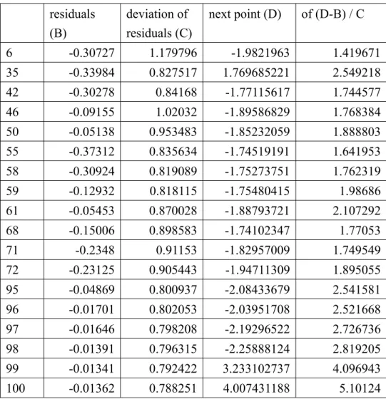
Table 3 shows the residual information of the set of {(xc, yc): c  I(n1)} and the deviations of the next point (x, y) obtained at Step 3 of 6th, 35th, 42nd, 46th, 50th, 55th, 58th, 59th, 61st, 68th, 71st, 72nd, 95th, 96th, 97th, 98th, 99th, and 100th stages within the 10th simulation run. The second and third columns record the mean value and the standard deviation of residuals of the set of {(xc, yc): c  I(n1)}, respectively. The fourth column presents the deviation of the next point (x, y). All of the last six next points are the identified outliers since they are in the last 25% and all ratios of their deviations are greater than 2.5.

Table 3: The residual information of the set of {(xc, yc): c  I(n1)} and the deviations of the next point (x, y) obtained at Step 3 of 6th, 35th, 42nd, 46th, 50th, 55th, 58th, 59th, 61st, 68th, 71st, 72nd, 95th, 96th, 97th, 98th, 99th, and 100th stages within the 10th simulation run.

residuals (B) deviation of residuals (C) next point (D) of (D-B) / C 6 -0.30727 1.179796 -1.9821963 1.419671 35 -0.33984 0.827517 1.769685221 2.549218 42 -0.30278 0.84168 -1.77115617 1.744577 46 -0.09155 1.02032 -1.89586829 1.768384 50 -0.05138 0.953483 -1.85232059 1.888803 55 -0.37312 0.835634 -1.74519191 1.641953 58 -0.30924 0.819089 -1.75273751 1.762319 59 -0.12932 0.818115 -1.75480415 1.98686 61 -0.05453 0.870028 -1.88793721 2.107292 68 -0.15006 0.898583 -1.74102347 1.77053 71 -0.2348 0.91153 -1.82957009 1.749549 72 -0.23125 0.905443 -1.94711309 1.895055 95 -0.04869 0.800937 -2.08433679 2.541581 96 -0.01701 0.802053 -2.03951708 2.521668 97 -0.01646 0.798208 -2.19296522 2.726736 98 -0.01391 0.796315 -2.25888124 2.819205 99 -0.01341 0.792422 3.233102737 4.096943 100 -0.01362 0.788251 4.007431188 5.10124

The following type-I and Type-II errors are adopted here to evaluate the performance of outlier detection: Type-I error is defined as the proportion of theoretical-non-outliers mis-specified as identified-outliers, and Type-II error is the proportion of theoretical-outliers mis-specified as identified-non-outliers.

Table 4 shows the mean value and the standard deviation of Type-I and Type II errors regarding the 100 simulation runs. As shown in Table 2, there are 60 runs with less than 6 theoretical outliers and 40 runs with at least 6 theoretical outliers. The results state that, without knowing the fitting function form associated with the data, we can use the proposed envelope procedure to identify the non-outlier with 98.17% correction rate and the outlier with 48.59% correction rate, respectively. Note that, if we do the outlier detection randomly without the knowledge of the fitting function

form, the Type-I and Type II errors is about 5% and 95% since on average there are 4.97 outliers in each set of 100 observations. In other words, the proposed envelope procedure contribute a 46.41% (= 95% - 48.59%) effect of outlier detection, which is significantly large.

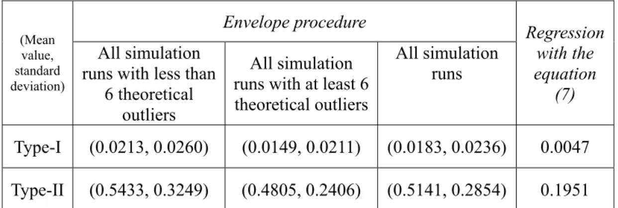
Table 4: The mean value and the standard deviation of Type-I and Type II errors regarding the 100 simulation runs.

(Mean value, standard deviation) Envelope procedure Regression with the equation (7) All simulation

runs with less than 6 theoretical

outliers

All simulation runs with at least 6 theoretical outliers

All simulation runs

Type-I (0.0213, 0.0260) (0.0149, 0.0211) (0.0183, 0.0236) 0.0047

Type-II (0.5433, 0.3249) (0.4805, 0.2406) (0.5141, 0.2854) 0.1951

The last column of Table 4 lists Type-I and Type II errors regarding the outlier detection via the non-linear regression method associated with equation (7). The last column of Table 4 states that when we know the fitting function form associated with the data, there are 99.53% of non-outliers identified correctly and 80.49% of outliers identified correctly. In other words, the results of Table 4 state that the knowledge of the fitting function form associated with the data contributes merely an extra 31.90% (= 80.49% - 48.59%) effect of outlier detection, compared with the proposed envelope procedure.

4. Discussion and Future works

In contrast with the resistant learning algorithm proposed by Tsaih & Cheng (2009) that uses a tiny ε value, this study proposes the envelope procedure with a non-tiny ε value that results in a nonlinear fitting function f around with the envelope

whose width being equal to 2ε. The envelope should contain at least n observations at the nth stage. This is distinct to the idea of Tsaih & Cheng (2009) that wants to evolve the fitting function to almost precisely fit all of n reference observations at the nth stage (because that the corresponding  value is tiny).

Furthermore, Tsaih & Cheng (2009) apply the deletion diagnostic mechanism to each reference observations to obtain its corresponding diagnostic quantity in Step 8 the resistant learning algorithm. The computation of such a deletion diagnostics is rather complicated and time-consuming when the size of the reference pool is large. In contrast, the proposed envelope procedure does not adopt such a deletion diagnostic mechanism. Therefore, the proposed envelope procedure has less computation than the resistant learning algorithm of Tsaih & Cheng (2009).

This study has conducted an experiment with 100 simulation runs, each of which has a different set of 100 observation data. The experiment results show without knowing the fitting function form associated with the data, we can use the proposed envelope procedure to identify the non-outlier with 98.17% correction rate and the outlier with 48.59% correction rate, respectively. Note that, if we do the outlier detection randomly without the knowledge of the fitting function form, the Type-I and Type II errors is about 5% and 95% since on average there are 4.97 outliers in each set of 100 observations. In other words, the proposed envelope procedure contribute a 46.41% (= 95% - 48.59%) effect of outlier detection, which is significantly large. It seems that the experimental result is positive.

In sum, this study has fulfilled the following objectives:

 Revise the resistant learning procedure of Tsaih and Cheng (2009) to form an effective way of identifying outliers in the context of robust nonlinear modeling.

 Set up a laboratory experiment to justify the effectiveness of the revised resistant learning procedure for identifying outliers in the context of robust nonlinear modeling.

Due to the complexity of the outlier detection in the context of robust nonlinear modeling, this study may be the first one in deriving an effective procedure for the outlier detection. Future works of this study are as follows:

 Set up a real-world experiment (regarding the finance or bioengineering applications) to explore the effectiveness of the proposed envelope procedure. More specifically, in the data-preprocessing stage, the envelope procedure is adopted to separate the training data into two subsets: one with the bulk and another with the (potential) outlier. In the modeling stage, the bulk data is used to tune the SLFN model via the back propagation learning algorithm (Rumelhart, Hinton and Williams 1986). In the forecasting stage, the obtained SLFN model is applied to the forecasting data to get corresponding predictions, based upon which decisions are made.

 Explore the reality of identified outliers in the real world experiment. That is, we want to explore some of the following questions: Are some of the identified outliers real outliers? Is there any further analysis of them that can help understand the way of detecting them and the way they affect the real world?

 Justify the necessity of data preprocessing mechanism for coping with outlier.

REFERENCES

1. Agyemang, M., Barker, K., and Alhajj, R. (2006). A comprehensive survey of numeric and symbolic outlier mining techniques, Intelligent Data Analysis, 10(6), 521–538.

2. Atkinson A (1985) Plots, Transformations and Regression. Oxford University Press, Oxford.

3. Atkinson A, Cheng T (1999) Computing Least Trimmed Squares Regression with the Forward Search. Statistics and Computing 9:251-263.

4. Atkinson A, Riani M (2002) Forward search added-variable t-test and the effect of masked outliers on model selection. Biometrika 89:939-946.

5. Beguin C, Chambers R, Hulliger B (2002) Evaluation of edit and imputation using robust methods. In Methods and Experimental Results from the Euredit Project, chapter 2, http://www.cs.york.ac.uk/euredit/.

6. Cook R D, Weisberg S (1982) Residuals and Influence in Regression. Chapman and Hall, London.

7. Dempster A, Gasko-Green M (1981) New tools for residual analysis. Annals of Statistics 9:945-959.

8. Hampel F, Ronchetti E, Rousseeuw P, Stahel W (1986) Robust Statistics: The Approach Based on Influence Functions. John Wiley, New York.

9. Hawkins S, He H, Williams G, Baxter R (2002) Outlier detection using neural networks. Proceedings of the 4th International Conference on Data Warehousing and Knowledge Discovery (DaWaK02), pp. 170-180.

10. Hoeting J, Raftery A, Madigan D (1996) A method for simultaneous variable selection and outlier identification in linear regression. Computational Statistics and Data Analysis 22:251-270.

11. Huber, J (1981) Robust Statistics, New York: John Wiley.

12. Hubert, M, Engelen, S (2007) Fast cross-validation of high-breakdown resampling methods for PCA. Computational Statistics and Data Analysis 51:5013-5024.

13. Knorr E, Ng R (1997) A unified approach for mining outliers. Proc. KDD, pp. 219-222.

14. Knorr E, Ng R (1998) Algorithms for mining distance-based outliers in large datasets. Proc. 24th Int. Conf. Very Large Data Bases, pp. 392-403.

15. Knorr E, Ng R, Tucakov V (2000) Distance-based outliers: Algorithm and applications. Very Large Data Bases 8:237-253.

16. Ronchetti, E, Field, C, Blanchard, W (1997) Robust linear model selection by cross-validation. Journal of the American Statistician Association, 92:1017–1023.

17. Rousseeuw P (1984) Least median of squares regression. Journal of the American Statistical Association 79:871-880.

18. Rousseeuw P, Leroy A (1987) Robust Regression and Outlier Detection. Wiley, New York.

19. Rousseeuw P, Van Driessen K (1999) Computing LTS Regression for Large Data Sets. Tech. Rep. University of Antwerp, Belgium.

20. Rumelhart D, Hinton G, and Williams R (1986) Modeling Internal Representations By Error Propagation. In: Rumelhart D, McClelland J (eds) Parallel Distributed Processing: Explorations in the Microstructure of Cognition,

21. Stromberg A (1993) Computation of High Breakdown Nonlinear Regression Parameters. Journal of the American Statistical Association 88:237-244.

22. Stromberg A, Ruppert D (1992) Breakdown in Nonlinear Regression. Journal of the American Statistical Association 87:991-997.

23. Sykacek P (1997) Equivalent error bars for neural network classifiers trained by Bayesian inference. Proceedings of the European Symposium on Artificial Neural Networks (Bruges, 1997), pp. 121-126.

24. Tsaih R (1997) The Reasoning Neural Networks. In: Ellacott S, Mason J, Anderson I (eds) Mathematics of Neural Networks: Models, Algorithms and Applications. Kluwer Academic publishers. London, page 367.

25. Tsaih R, Cheng, T (2009) A Resistant Learning Procedure for Coping with Outliers. Annals of Mathematics and Artificial Intelligence, 57(2): 161-180. 26. Williams G, Baxter R, He H, Hawkins S, Gu L (2002) A comparative study of

RNN for outlier detection in data mining. Proceedings of the 2nd IEEE

International Conference on Data Mining (ICDM02), pp. 709-712.

27. Windham M (1995) Robustifying model fitting. Journal of the Royal Statistical Society 57(B):599-609.

28. Zaman A, Rousseeuw P, Orhan M (2001) Econometric Applications of High-Breakdown Robust Regression Techniques. Econometrics Letters 71:1-8.

國科會補助專題研究計畫項下出席國際學術會議心得報告

一、參加會議經過

本人於 2012 年 6 月 9 日半夜搭乘華航飛機，於澳洲時間 6 月 10 日早上抵達布

里斯本，當天下午即前往研討會場地辦理註冊，由於報告的時間是 6 月 12 早上，所

以與會的前兩天我皆有參與早上舉行的 plenary lecture，和 International Joint

Conference on Neural Networks (IJCNN)的 lecture，並旁聽多場有興趣的

Sessions，以及觀摩 poster 場次。6 月 12 日早上 poster 的時間為 10:20-12:00，

發表過程順利，嘗試回答觀摩學者們所提出的疑問，並與學者們交換心得，獲益良

多，下午繼續參與兩場 open lectures，於 6 月 12 日半夜 12:00 左右搭乘華航飛機

計畫編號

NSC-98-2410-H-004-049-MY2

計畫名稱

財務報表舞弊探索與類神經網路

出國人員

姓名

黃馨瑩

服務機構

及職稱

政治大學資訊管理系博士班五年級

會議時間

2012 年 6 月 10 日

至

2012 年 6 月 12 日

會議地點 澳洲布里斯本

會議名稱

(中文) 2012IEEE 電腦智慧國際會議

(英文) 2011IEEE Computational Intelligence Society

發表論文

題目

(中文) 應用增長層級式自我組織映射網路於預測之途徑

(英文) The Prediction Approach with Growing Hierarchical

Self-Organizing Map

由布里斯本返回台灣。

二、與會心得

我是資訊管理系蔡瑞煌老師的博士班學生黃馨瑩，這是我於博士班階段第五次

出國參與國際研討會，上一次參加 WCCI 研討會是 2008 年我博二的時候，很高興再

次有這樣的機會參加 2012 年 WCCI 研討會，希望能把握這次發表的經驗，把自己目

前的研究議題在發表的機會中與其他學者們分享。WCCI 研討會每兩年舉辦一次，主

要專注在電腦智慧的研究領域，是規模相當大的類神經網路、演化式計算、機器學

習以及 AI 相關的聯合國際會議，主辦單位邀請了很多學術界知名的學者分享其研究

成果和對當前研究議題的看法，與會人員大多是博士生以及助理教授以上的學者先

進，因此我透過觀摩學者的發表接收到了很多不同的刺激與心得，在 poster 發表的

過程中，我向多位學者介紹 GHSOM 的運作原理，和進行預測的方法，很高興有被一

位學者稱讚 poster 做得不錯，並與一位 Juyang Weng 學者交流對於 SOM 裡 neuron

之互動機制的看法，Juyang Weng 認為 neuron 之互動應為雙向的，也就是有反饋，

且為了模擬人類腦部運作，neuron 之間的聯結是沒有距離限制的，所以 SOM 的

neighborhood function 有改善的空間，此外每個 neuron 就像 agent 般，有自己的

memory 和簡單的運作原則，因此這方面的學門需要眾多領域的合作，如資訊、電機、

神經科學、心理學等。在交流的過程中我獲得許多啟發，認為從 poster 的發表中能

獲得更多與學者們互動的機會，並擁有較長時間的曝光機會，例如當天下午我參與

一場 open lecture 時就有學者與我打招呼說早上有看到我的 poster，我們有簡單交

流並交換名片。

隨著參與國際研討會的經驗累積，我更懂得從學者們展現的研究成果中擷取值

得學習的 idea，並也嘗試在 poster 場次中，對有興趣的論文佇足觀摩，並進一步向

作者發問與交流，得到更多研究方法上的啟發。

因此能和與會所認識的學者們交流，聆聽以及觀摩其他學者的研究成果是難得

的機會，在參與國際會議的經驗中我也了解了現在相關研究議題的趨勢變化，進而

發覺目前自己研究的改進空間和未來發展方向，非常感謝有這樣的機會能與國際學

者交流，以及藉機體驗布里斯本的當地風情。

時間：2012/6/12 地點：International Convention Center, Brisbane, Australia.

三、考察參觀活動(無是項活動者略)

略

四、建議

無

五、 攜回資料名稱及內容

 大會議程：2012 IEEE World Congress on Computational Intelligence,10-15,

June, 2012 一本

 大會 USB 隨身碟一個

六、其他

無

來源:

Kate Smith-Miles <ijcnn2012@ieee-cis.org>

收信: 96356511@nccu.edu.tw , tsaih@mis.nccu.edu.tw

標題: IJCNN 2012 Paper #462 Decision Notification

日期: 21 Feb 2012 18:34:18 -0000

Dear Author(s),

Congratulations! On behalf of the IJCNN 2012 Program Chairs, we are pleased to inform you that your paper:

Paper ID: 462

Author(s): Shin-Ying Huang and Rua-Huan Tsaih

Title: The Prediction Approach with Growing Hierarchical Self-Organizing Map

has been accepted for presentation at the 2012 International Joint Conference on Neural Networks and for publication in the conference proceedings published by IEEE. This email provides you with all the information required to complete your paper and submit it for inclusion in the proceedings. A notification of the presentation format (oral or poster) and timing of that presentation will be sent in a subsequent email.

Here are the steps:

1. Please address the attached REVIEWERS' COMMENTS which are intended to improve the final manuscript. Final acceptance is conditional on appropriate response to the requirements and comments.

2. Please prepare your manuscript for final camera ready submission by

following the formats described on the conference web site and using the IEEE templates:

http://www.ieee-wcci2012.org

Once you are ready to submit it, please go to:

to submit your final camera-ready paper. On this page you will need to use the following password:

hb8z8h49f

Please do adhere the strict deadline for final manuscript submission April 2, 2012. Any papers submitted after this date will not be included in the

proceedings. The paper must be re-submitted even if the reviewers indicated that no changes are required.

3. In order for your paper to be published in the conference

proceedings, a *signed IEEE Copyright Form* must be submitted for each paper. IJCNN 2012 has registered to use the IEEE Electronic Copyright (eCF) service. The confirmation page shown after submitting

your final paper contains a button linking directly to a secure IEEE eCF site which allows electronic completion of the copyright assignment process. In case it fails, please have the completed IEEE Copyright

Form, found at http://www.ieee.org/web/publications/rights/copyrightmain.html, emailed it to Publication Co-Chair, Daryl Essam (d.essam@adfa.edu.au).

IMPORTANT: No paper can be published in the proceedings without being accompanied by a Completed IEEE Copyright Transfer Form. You must complete and submit this form to have your paper included in the conference proceedings.

4. Register for the conference at http://www.ieee-wcci2012.org by clicking on the conference registration link on the right-hand side of the main page.

IMPORTANT: Each paper must have a corresponding registered author to be included in the proceedings. Papers that do not have an associated registered author will not be included in the proceedings. The deadline for author registration is April 2, 2012 so be sure to register by that time to ensure that your paper is included in the proceedings. Please ensure that you complete your registration early.

If you have any questions regarding the reviews of your paper please contact Kate Smith-Miles <ijcnn2012@ieee-cis.org>.

Sincerely, Kate Smith-Miles <ijcnn2012@ieee-cis.org>

REVIEWERS' COMMENTS

--- REVIEW NO. 1

Originality: Weak Accept Significance of topic: Accept Technical quality: Weak Accept

Relevance to IJCNN 2012: Weak Accept Presentation: Accept

Overall rating: Weak Accept

Reviewer's expertise on the topic: High Suggested form of presentation: Poster Best Paper Award nomination: No

Comments to the authors:

The study consists of an application of the Growing Hierarchical Self-organizing Map to the problem of

financial statement fraud detection. The issue addressed is of clear practical importance, at to date, there

have been few (if any) applications of GHSOM for this task.

The paper is quite clearly-written and is fairly easy to follow.

The primary drawback of the paper is that the results of the study are not benchmarked against any other

method (obviously many traditional methods of classification exist). Therefore, the reader cannot form any

real view as to whether the method applied actually produces good in/out sample results. Consequently,

--- REVIEW NO. 2

Originality: Neutral

Significance of topic: Neutral Technical quality: Weak Reject Relevance to IJCNN 2012: Accept Presentation: Weak Reject

Overall rating: Neutral

Reviewer's expertise on the topic: Medium Suggested form of presentation: Poster Best Paper Award nomination: No

Comments to the authors: Contributions

In this paper, the Growing Hierarchical Self-Organizing Map (GHSOM) was applied as a prediction tool for financial fraud detection (FFD), based on the

assumption that there was a certain spatial relationship amongst fraud and non- fraud samples. By comparing the results based on training samples and testing samples, the authors concluded that the prediction performance was

acceptable.

Positive aspects

This is a new application of GHSOM to FFD, though the advantages of proposed method have not been well demonstrated by the results.

Observed deficiencies and suggestions

The entire study in this paper was based on the assumption that there was a certain spatial relationship amongst fraud and non-fraud samples. However, there was a lack of theoretical foundation for such assumption. A citation should be provided if such assumption has been applied in literature, or a further explanation should be given.

The advantage of GHSOM over SOM was mentioned in the Introduction. Unfortunately it was not tested or demonstrated by the experiment results.

Lack of supporting evidences for final results, why error lower than

20% is considered to be acceptable? Comparing to whom? Or based on what criterion?

Was the parameter beta adjusted based on the classification error? If yes, whether or how this parameter can be adapted in new datasets?

Any limitation of the proposed approach?

There was no definition for FT and NFT. There was no definition for Type I and Type II error.

The conclusion repeats some content already used.

Repeated typo. "spacial" should be "spatial"?

--- REVIEW NO. 3

Originality: Accept

Significance of topic: Weak Accept Technical quality: Accept

Relevance to IJCNN 2012: Accept Presentation: Accept

Overall rating: Weak Accept

Reviewer's expertise on the topic: Low Suggested form of presentation: Any Best Paper Award nomination: No

Comments to the authors:

The paper goes into great detail of the methodology. My main criticism is that the cost of a type I error and a type II error are different, so summing the two is not optimal. It is not clear whether the method is superior to existing methods of identifying fraud, because no comparison is made.

The Prediction Approach with Growing Hierarchical

Self-Organizing Map

Shin-Ying Huang

Department of Management Information Systems National Chengchi University

Taipei, Taiwan

Rua-Huan Tsaih

Department of Management Information Systems National Chengchi University

Taipei, Taiwan

Abstract— The competitive learning nature of the Growing

Hierarchical Self-Organizing Map (GHSOM), which is an unsupervised neural networks extended from Self-Organizing Map (SOM), can work as a regularity detector that is supposed to help discover statistically salient features of the sample population. With the spatial correspondent assumption, this study presents a prediction approach in which GHSOM is used to help identify the fraud counterpart of each non-fraud subgroup and vice versa. In this study, two GHSOMs— a non-fraud tree (NFT) and a fraud tree (FT) are generated via the non-fraud samples and the fraud samples, respectively. Each (fraud or non-fraud) training sample is classified into its belonging leaf nodes of NFT and FT. Then, two classification rules are tuned based upon all training samples to determine the associated discrimination boundary within each leaf node, and the rule with better classification performance is chosen as the prediction rule. With the spatial correspondent assumption, the prediction rule derived from such an integration of FT and NFT classification mechanisms should work well. This study sets up the experiment of fraudulent financial reporting (FFR), a sub-field of financial fraud detection (FFD), to justify the effectiveness of the proposed prediction approach and the result is quite acceptable.

Keywords: Fraudulent Financial Reporting; Growing Hierarchical Self-Organizing Map; Unsupervised Neural Networks; Classification; Financial Fraud Detection

I. THEPREDICTION AND THEGHSOM Artificial Neural Network (ANN) is one of the data mining techniques, which plays an important role in accomplishing the task of financial fraud detection (FFD) that involves distinguishing fraudulent financial data from authentic data, disclosing fraudulent behavior or activities, and enabling decision makers to develop appropriate strategies to decrease the impact of fraud [20]. Amongst the ANN applications to FFD, Self-Organizing Map (SOM) [17] is adopted a lot in diagnosing bankruptcy [6]. The major advantage of SOM is its great visualization capability of topological relationship amongst the high-dimensional inputs in the low-dimensional view. To address the issue of fixed network architecture of SOM through developing a multilayer hierarchical network structure, the Growing Hierarchical Self-Organizing Map (GHSOM) [8][9][23] has been developed. The flexible and hierarchical features of GHSOM generate more delicate clustering results than SOM and make GHSOM a powerful and versatile analysis tool. GHSOM has been used in many fields

such as image recognition, web mining, text mining, and data mining [8][9][23][25][26][29] as a useful clustering tool for further feature extraction. Few of researches have applied GHSOM to the prediction tasks [12][14][20]. This motivates this study develop a prediction approach in which GHSOM is used to help identify the fraud counterpart of each non-fraud subgroup and vice versa.

Specifically, this study assumes that there is a certain spatial relationship amongst fraud and non-fraud samples. For instance, if a group of fraud samples and their non-fraud counterparts are identical, each cluster of fraud samples tend to be located separately from the non-fraud samples. In other words, the spatial distributions of most fraud samples and their non-fraud counterparts are the same. If such a spatial relationship amongst fraud and non-fraud samples does exist, we hope that the GHSOM can help to identify the fraud counterpart of each subgroup of non-fraud samples and vice versa. Such idea of combining supervised and unsupervised learning approach can inspire the model design and improve the classification accuracy. For example, Carlos (1996) applied SOM to financial diagnosis by developing a DSS for the analysis of accounting statements, which includes Linear Discriminant Analysis (LDA) and Multilayer Perceptron (MLP) to delimit the solvency regions within the SOM. Such approach is based on the idea that the unsupervised neural models must be complemented with a statistical study of the available information.

To practically explore such a spatial correspondent assumption, this study derives a prediction approach based upon the GHSOM. To justify such a prediction approach, we set up the fraudulent financial reporting (FFR) experiment.

The remainder of this paper is organized as follows. A review of relevant literature is shown in Section II. Section III presents the proposed approach. Section IV reports the experimental design of FFR. The last section concludes with a summary of findings, implications, and future works.

II. LITERATURE REVIEW

A. Growing Hierarchical Self-Organizing Maps

The training process of GHSOM consists of the following four phases [8]:

y Initialize the layer 0: The layer 0 includes single node whose weight vector is initialized as the expected value of all input data. Then, the mean quantization error of layer 0 (MQE0) is calculated. The MQE of a node

denotes the mean quantization error that sums up the deviation between the weight vector of the node and every input data mapped to the node.

y Train each individual SOM: Within the training process of an individual SOM, the input data is imported one by one. The distances between the imported input data and the weight vector of all nodes are calculated. The node with the shortest distance is selected as the winner. Under the competitive learning principle, only the winner and its neighborhood nodes are qualified to adjust their weight vectors. Repeat the competition and the training until the learning rate decreases to a certain value. y Grow horizontally each individual SOM: Each individual

SOM will grow until the mean value of the MQEs for all of the nodes on the SOM (MQEm) is smaller than the

MQE of the parent node (MQEp) multiplied by τ1 as

stated in (1). If the stopping criterion is not satisfied, find the error node that owns the largest MQE and then, as shown in Fig. 1, insert one row or one column of new nodes between the error node and its dissimilar neighbor.

MQEm < τ1 × MQEp (1)

Figure 1. Horizontal growth of individual SOM. The notation x indicates the error node and y for the dissimilar neighbor

y Expand or terminate the hierarchical structure: The node with an MQEi greater than τ2 × MQE0 will develop a next

layer of SOM. In this way, the hierarchy grows until all of the leaf nodes satisfy the stopping criterion stated in (2).

MQEi < τ2 × MQE0 (2)

GHSOM has been used in fields of image recognition, web mining, text mining, and data mining. For example, [25] had shown the feasibility of using GHSOM and LabelSOM techniques in legal research by tests with text corpora in European case law. GHSOM was used to present a content-based and easy-to-use map hierarchy for Chinese legal documents in the securities and futures markets [26]. Reference [1] used GHSOM to analyze a citizen web portal and provided a new visualization of the patterns in the hierarchical structure.

Not many studies have applied GHSOM in the purpose of forecasting until recent years. For instance, a two-stage architecture with GHSOM and SVM was employed by [14] to better predict financial indices. GHSOM was applied with support vector regression model to product demand forecasting [20]. In [12], GHSOM was integrated into case-based reasoning system in design domain.

B. Fraudulent financial reporting

FFR is a kind of financial fraud that involves the intentional misstatement or omission of material information from an organization’s financial reports [4]. FFR can lead not only to significant risks for stockholders and creditors, but also financial crises for the capital market [3]. Prior FFR related studies showed that the main data mining techniques used for FFD are logistic models, neural networks, the Bayesian belief network, and decision trees. These data mining techniques also contribute to the FFR detection. For example, [11] applied the back-propagation neural network to FFR detection. The model used five ratios and three accounts as input. The results showed that the back-propagation neural network had significant capabilities when used as a fraud detection tool. Reference [10] proposed a generalized adaptive neural network algorithm, named AutoNet to detect FFR and compared their model against the linear and quadratic discriminant analysis and logistic regression. They concluded that AutoNet is more effective at detecting fraud than standard statistical methods. For a broader financial fraud detection domain, [21] have done a classification framework and an academic review of literature which used data mining techniques in FFD.

III. THE PROPOSED PREDICTION APPROACH

The proposed prediction approach consists of the following three phases: the training, modeling, and predicting. Table I shows the training phase, in which the task of data preprocessing is done via step 1 and step 2. Step 2 can apply any variable selection tool such as discriminant analysis, logistic model, and so forth.

TABLE I. THE TRAINING PHASE.

In the training phase, we want to use GHSOM to classify fraud and non-fraud samples respectively in such a way that the spatial relationship amongst fraud and non-fraud samples can be explicitly identified later. Thus, before processing step 3, the training samples are grouped as the fraud ones and the non-fraud ones. In step 3, the non-fraud samples are used to generate an acceptable GHSOM named FT (fraud tree). After identifying the FT, the values for (GHSOM) parameters breadth (τ1) and

depth (τ2) are determined and stored in step 4. Then, in step 5,

the determined values of τ1 and τ2 and the non-fraud samples

are used for setting up another GHSOM named NFT (non-fraud tree). With the spatial correspondent assumption and the same setting of training parameters (τ1 and τ2) of GHSOM,

each leaf node of NFT may have one or more than one counterpart leaf nodes in FT and vice versa despite FT and NFT are established based on fraud and non-fraud samples,

step 1: Sample and variable measure.

step 2: Identify the significant variables that will be used as the input variables.

step 3: Use the fraud samples to generate an acceptable GHSOM named FT.

step 4: Based upon the accepted FT, determine the (GHSOM training) parametersbreadth (τ1) and depth (τ2).

step 5: Use the non-fraud samples and the determined parameters τ1 and τ2 to generate another GHSOM named NFT.