藉由改變巨方塊中資料運算的順序以提升去方塊濾波器的效能

全文

(1)國立交通大學電機學院 IC 設計產業研發碩士班碩士論文. 藉由改變巨方塊中資料運算的順序以提升去方塊濾波器的效能 Reordering the data operation of macro-block for improving the performance of de-blocking filter in H.264/AVC. 研究生：陳泰霖指導教授：鍾崇斌. 教授. 中華民國九十七年十月.

(2) 藉由改變巨方塊中資料運算的順序以提升去方塊濾波器的效能 Reordering the data operation of macro-block for improving the performance of de-blocking filter in H.264/AVC. 研究生：陳泰霖. Student：Tai-Lin Chen. 指導教授：鍾崇斌. Advisor：Chung-Ping Chung. 國立交通大學電機學院 IC 設計產業研發碩士班碩士論文. A Thesis Submitted to College of Electrical and Computer Engineering National Chiao Tung University in partial Fulfillment of the Requirements for the Degree of Master in. Industrial Technology R & D Master Program on IC Design June 2008 Hsinchu, Taiwan, Republic of China. 中華民國九十七年十月.

(3) 藉由改變巨方塊中資料運算的順序以提升去方塊濾波器的效能學生:陳泰霖. 指導教授:鍾崇斌. 國立交通大學電機學院產業研發碩士班. 摘. 要. ISO/IEC as MPEG-4 Part 10 Advanced Video Coding(AVC) 與 ITU-T 制定之 H.264/AVC 是最新的視訊國際壓縮標準。H.264/AVC 具有較高的視訊壓縮率以及能提供較佳視訊品質。由於 H.264 是採用方塊(block)模式去做影像處理，所以也同時造成了影像的失真，當中最明顯的就是方塊雜訊效應(blocking artifact)。為了解決這個問題，在 H.264/AVC 的視訊標準裡有一個功能方塊稱作去方塊濾波器(de-blocking filter)，根據 H.264/AVC 解碼器的複雜度模擬結果中，結果顯示去方塊濾波器是解碼器內最複雜的部分，大約佔用了 36%的執行時間。由於去方塊濾波器的資料處理過程中有重複存取的現象產生，因此為了有效提升記憶體存取效能及去方塊濾波之執行速度，我們提出一種新的架構給 H.264/AVC 的去方塊濾波器使用。首先我們提出了一個新的資料運算順序，使得濾波的時間以及記憶體的使用較傳統的設計少。並提出一個新的資料存取方式，讓去方塊濾波器在處理過程中能夠同時存取所需的資料，藉此來減少所需的工作週期。我們使用硬體描述語言(Verilog Hardware Description Language)來設計此架構, 再利用模擬軟體(ModelSim)分別驗證其功能，並在台灣積體電路公司(TSMC)所提供的 0.13μm 製程 library 及 Synopsys 所提供的合成軟體做合成電路，其合成的結果顯示，在時脈速度為 100MHz 的情況下，所提出的去方塊濾波器架構能夠處理解析度為 720P(1280×720 @60fps)的高解析度視訊影像。. i.

(4) Reordering the data operation of macro-block for improving the performance of de-blocking filter in H.264/AVC Student：Tai-Lin Chen. Advisor：Dr. Chung-Ping Chung. Industrial Technology R & D Master Program of Electrical and Computer Engineering College National Chiao Tung University. ABSTRACT H.264/AVC is a new generation video coding standard and is approved by ITU-T as Recommendation H.264 and by ISO/IEC as MPEG-4 Part 10 Advanced Video Coding. H.264/AVC is to achieve higher compression efficiency and provide the better video quality. Because the H.264 is an adoption block the mode does image processing. However, the most annoying artifact known as the blocking artifact also comes into existence. In order to solve this problem, the de-blocking filter is an important component of H.264/AVC to reduce the block artifacts. In the complexity simulation of H.264/AVC decoder part, the de-blocking filter is the most complexity part, probably has taken 36% execution time. Because of in the de-blocking filter data processing process has the repetition access appearance. In order to improve memory performance and speed up the de-blocking filter, we propose a new architecture for de-blocking filter in H.264/AVC. First we propose a novel filtering order that results in significant saving in both filtering time and local memory usage. And we propose a new data access a method. Let the de-blocking filter can simultaneous access necessity the data in processing process, we can reduce the working cycles. The proposed architecture is synthesized with TSMC 0.13μm technology. The synthesized de-blocking filter architecture could process video in 720P HD (High-definition television, HDTV, 1280×720 pixels/frame, 60 frames/sec video signals) format at 100MHz. ii.

(5) 誌謝終於結束了漫長的碩士求學生涯，這三年來的求學生涯對我來說實在是畢生難忘，而在此要跟長期陪伴我度過這段時間的所有人說一聲謝謝。這篇論文得以完成，首先要感謝的是我的指導教授鍾崇斌老師，鍾老師豊富的研究經驗且鼓勵我們自發性的學習，且當在我論文研究時，常常提出很好的建議，讓我在研究所兩年中，學習到解決、發現問題的方法，也學到了許多非常有用的知識。並且在這裡感謝單智君老師、邱日清老師、洪士灝老師，在百忙之中願意參加我的口試，並且在口試過程中提出許多寶貴的意見，使我的論文能夠更加的完善。同時感謝蔣昆成學長，這三年來的熱心指導，在研究過程中不斷的提供許多寶貴的意見，使我能夠更準確的達到研究目的，此外也感謝我週遭的同學與朋友，不管在課業上或是日常生活上能夠一起扶持與成長。最後要感謝我的父母親，願意支持我繼續唸碩士班的決定，並且在我求學的這段時間內不斷的加油打氣，如果沒有你們的支持，我相信我是無法順利完成學業的，謝謝你們。. iii.

(6) List of Contents 中文摘要英文摘要誌謝目錄表目錄. ……………………………………………………………………………i ……………………………………………………………………………ii ……………………………………………………………………………iii ……………………………………………………………………………iv ……………………………………………………………………………vi. 圖目錄一、 1.1 1.2 二、. ……………………………………………………………………………viii Introduction………………………………………………………………1 Motivation…………………………………………………………………3 Objective……………………………………………………………………4 Background & Related Work………………………………………………5. 2.1 2.2. The blocking artifact………………………………………………………5 De-blocking Filter Algorithm………………………………………………6 2.2.1 2.2.2. Input of the de-blocking filter………………………………………………7 De-blocking Filter Processing Order………………………………………8 Boundary Strength…………………………………………………………11. 2.3.1 2.3.2 2.4.1 2.4.2. Gradient of image samples across the boundary…………………………13 Derivation process for the thresholds for each block edge………………15 Filtering Operation………………………………………………………16 Normal mode : ( Bs=1~3 ) ………………………………………………16 Stronger mode : ( Bs=4 ) …………………………………………………19. 2.5.1 2.5.2 2.5.3 2.5.4. Related Work……………………………………………………………22 Basic Processing Order……………………………………………………23 Advanced Processing Order………………………………………………24 2-D Processing Order………………………………………………………25 2-D Simultaneous Processing Order………………………………………26. 2.3. 2.4. 2.5. 2.5.5. Summary related work……………………………………………………27 Proposed architecture of de-blocking filter………………………………28 Overview of the Proposed Architecture……………………………………28 Filtering Order……………………………………………………………30. 3.2.1. De-blocking filter order of the 4×4 sub-block edge………………………30. 3.2.2 3.2.3 3.4. Proposed edge filtering order………………………………………………31 Divide the luma block……………………………………………………32 Parallel Memory Unit………………………………………………………33 Data Buffer ＆ Transpose Buffer …………………………………………34. 3.5. Control Unit………………………………………………………………36. 三、 3.1 3.2. 3.3. iv.

(7) 四、 4.1 4.2 4.3 五、 Reference. Implementation results……………………………………………………46 The simulation environment………………………………………………46 Comparison with other architectures………………………………………47 Future work………………………………………………………………50 Conclusion…………………………………………………………………51 ……………………………………………………………………………52. v.

(8) List of Figures Fig 1.1 Block diagram of H.264/AVC…………………………………………………………3 Fig 1.2 Run-time profile of H.264/AVC decoder……………………………………………4 Fig 2.1 Illustration of blocking artifact………………………………………………………6 Fig 2.2 The location of de-blocking filter in H.264/AVC decoder……………………………7 Fig 2.3 Input of the de-blocking filter…………………………………………………………8 Fig 2.4 Horizontal filtering across luma vertical edges………………………………………9 Fig 2.5 Vertical filtering across luma horizontal edges………………………………………10 Fig 2.6 Filtering process of chroma block……………………………………………………10 Fig 2.7 Flowchart of Bs deriving process……………………………………………………11 Fig 2.8 Bs value for horizontal filtering across vertical edges………………………………12 Fig 2.9 Bs value for vertical filtering across horizontal edges………………………………13 Fig 2.10 Gradient of image samples across the boundary……………………………………14 Fig 2.11 Normal mode operations for luminance block……………………………………16 Fig 2.12 Normal mode operations for chrominance block…………………………………17 Fig 2.13 Stronger mode operations for luminance block……………………………………19 Fig 2.14 Stronger mode operations for chrominance block…………………………………20 Fig 2.15 Flow chart of filtering process………………………………………………………21 Fig 2.16 Basic processing order ……………………………………………………………23 Fig 2.17 Advanced processing order…………………………………………………………24 Fig 2.18 2-D processing order………………………………………………………………25 Fig 2.19 2-D simultaneous processing order…………………………………………………26 Fig 3.1 System architecture of the de-blocking filter…………………………………………28 Fig 3.2 De-blocking filter order of the 4×4 sub-block edge…………………………………30 vi.

(9) Fig 3.3 Proposed filtering order………………………………………………………………31 Fig 3.4 Luma block of the filtering order……………………………………………………32 Fig 3.5 Luma block break down upper and the lower two parts……………………………32 Fig 3.6 Memory mapping of 4×4 blocks……………………………………………………33 Fig 3.7 for example a 4×4 block……………………………………………………………34 Fig 3.8 Data buffer operation…………………………………………………………………35 Fig 3.9 Transpose buffer operation…………………………………………………………36 Fig 3.10 Overall architecture of our proposed de-blocking filter……………………………37 Fig 3.11 The data path of storing block of L1 and L2 into data buffer………………………37 Fig 3.12 Horizontal filtering on vertical edge 1………………………………………………38 Fig 3.13 Horizontal filtering on vertical edge 2………………………………………………39 Fig 3.14 Horizontal filtering on vertical edge 3………………………………………………39 Fig 3.15 The data path of storing block of T1 and T2 into data buffer………………………40 Fig 3.16 Vertical filtering on horizontal edge 4………………………………………………41 Fig 3.17 Vertical filtering on horizontal edge 5………………………………………………41 Fig 3.18 The data path of storing block of B2 and B6 into data buffer………………………42 Fig 3.19 Horizontal filtering on vertical edge 6………………………………………………43 Fig 3.20 The data path of storing block of T3 and T4 into data buffer………………………43 Fig 3.21 vertical filtering on horizontal edge 7………………………………………………44 Fig 3.22 vertical filtering on horizontal edge 8………………………………………………45 Fig 4.1 Design flow in our implementation…………………………………………………46. vii.

(10) List of Tables Table 2.1 Determining of boundary strength…………………………………………………12 Table 2.2 Derivation of indexA and B from offset dependent threshold variable α and β…15 Table 2.3 Value of filter clipping variable t C 0 as a function of indexA and Bs……………18 Table 2.4 comparison of above proposed architecture………………………………………27 Table 3.1 data flow of our proposed architecture……………………………………………45 Table 4.1 Comparison of hardware cost in the main module………………………………47 Table 4.2 Performance comparison of various architectures…………………………………48 Table 4.3 implementation of our proposed…………………………………………………49. viii.

(11) Chapter 1 Introduction. The Joint Video Team (JVT) is composed by ITU-T Video Coding Experts Group (VCEG) and ISO/IEC Moving Picture Experts Group (MPEG). JVT formulates a new video compression standard is H.264/AVC [1]. The main objectives of H.264/AVC are to develop a set of high efficient, the network-friendly and error-resilient ability. The video compression standard provides from the mobile phone to HDTV widespread application and improves largely rate-distortion efficiency. H.264 was compared to the existing standards such as MPEG-2, H.263++ (Annexes DFIJT) and MPEG-4, in similar regards under the video compression quality to be possible to save approximately 50% above bit-rate [3].. Although the encoding efficient of H.264/AVC is higher than the video encoding standard formerly, but it have the quite complex encoding technology and the mode choice, so its operation order complexity also far to be higher than the encoding standard actually formerly. These improved characteristics are due to the application of several new coding tools within the compression process defined by the standard, such as multi-mode intra-prediction, multi-frame variable-block-size, variable block-size motion estimation, quarter-pixel motion compensation, inter-prediction, integer discrete cosine transform (DCT), context adaptive binary arithmetic coding (CABAC) and in-loop de-blocking filtering. Each of these new encoding techniques contributes more or less to the total gain of whole H.264/AVC system in compression ratio, but also increased its operation order complexity.. 1.

(12) One of the most special features in H.264/AVC is de-blocking filtering. Because of the characteristic of H.264/AVC encoding compression calculation method sometimes has obviously the block artifacts phenomenon, such as block-based motion compensated prediction, intra prediction, and integer discrete cosine transform [4]. The de-blocking filter contributes to eliminate or diminish the block artifacts in the decoded video sequence, while producing the same objective quality as the non-filtered video, that can reduces the bit-rate typically by 5%~10% [3]. But due to the de-blocking filter operations irregular data access and uses inner loop of the highly optimized filtering algorithm. Thus the de-blocking operation accounts consuming one-third of the computational complexity of H.264/AVC decoder [6].. There are two different schemes of De-blocking filter in video codec, post filter and in-loop filter. In the case of post filter, the filter is only operation on the display buffer outside the coding or decoding loop. The decoded data is stored in a data buffer, filtered and then stored in another video buffer before being forwarded to the display device [5]. Thus the post filter is not normative in the standardization process. As shown in figure 1.1, the in-loop filter is placed inside the coding loop. So that the in-loop filter processed frames are used as reference frames for motion compensation of subsequent coded frames [4]. Thus the in-loop filter is normative in the standardization process, in order to stay in synchronization with the encoder.. There are several advantages of in-loop filter over post filter, one the advantage is that no need for an extra frame buffer in the decoder, and that can improves quality of video streams and significant reduction in decoder complexity compared to post filtering [4], and the in-loop filter reduces the bit rate than the post filter.. 2.

(13) Figure 1.1: Block diagram of H.264/AVC. 1.1 Motivation The De-blocking Filter of H.264 decoder is an important part of entire system; it can dominate system performance and quality for video image due to high computing complexity and real-time application. Figure 1.2 shows the profiling results of a decoding process, the de-blocking Filter consume 36.05% of total decoding time [7], so the processing time becomes very important. We can opportunity of processing order of current De-blocking Filter that many image data would be re-access between external memory and internal SRAM [8], and it spends many cycles to transpose the image data.. 3.

(14) Deblocking Filter Interprediction. 36.05%. Inverse Transform and Inverse Quantization 38.92%. 9.32%. Entropy Decoding Intraprediction. 8.61% 5.89%. Others 1.21%. Figure 1.2: Run-time profile of H.264/AVC decoder. 1.2 Objective In order to solve the problem about the number of accesses of the external memory, we proposed the processing order of de-blocking Filter and an efficient architecture of the filter. Because of ours design methods that can accelerate filtering process with pipeline technique for reducing the internal memory size and using fewer the register amounts.. 4.

(15) Chapter 2 Background and Related Works In this chapter, we will describe the block artifacts occur and the algorithm of de-blocking filter in H.264/AVC. Second, we will introduce some de-blocking filter processing order to sample processing level.. 2.1. The blocking artifact The majority video compression standard uses that the JPEG related compression. technique to use in spatial the redundancy. In JPEG, divided into many 8×8 block for video and it uses the discrete cosine transforms (DCT) to make each block the transformation. After process transformation, the transformed coefficients are quantized then entropy coded. Then it makes the classification by transformed coefficients use to the quantization table the inside quantization step. The quantization table design reserves more low frequency coefficient and less high frequency coefficient. Under the low bit rates condition, the possibility reserve only one Direct Coefficient (DC) and some Alternate Coefficient (AC) represents a block. Therefore we may lose the relativity of neighboring block. As a result, the reconstruction image or video quality will be influenced by obvious factitiousness. This is the blocking artifact as shown in figure 2.1.. Blocking artifact factors of H.264/AVC : (1) The intra and inter frame prediction error coding of H.264/AVC use the integer discrete cosine transforms (DCT). The transform coefficients are too rough that can produce visually disturbing discontinuities phenomenon at the block boundaries [4].. 5.

(16) (2) Second factor is motion compensated prediction. The motion compensated blocks are produced by copying interpolated pixel data that possible in the different locations of the different reference frames [4]. Because this reason, therefore we can not find the appropriate data that have discontinuities phenomenon at the block edge.. Figure 2.1: Illustration of blocking artifact. 2.2. De-blocking Filter Algorithm In H.264/AVC applies in-loop de-blocking filter to used eliminate blocking artifact then. generates a smooth frame as shown in figure 2.2. The intra and inter frame prediction error coding are transformed then quantized. After decoding procedure, the reconstruction block has an error with the originally block. Therefore it has not the continual phenomenon then can again the block edge production. In order to eliminate discontinuity situation, the process is applied.. First the de-blocking filter divides a frame many macro-block and the de-blocking filter processing unit is a macro-block. After first a complete processing current macro-block, the next macro-block is just sent in. After first a complete processing current frame, the next 6.

(17) frame is just sent in. The de-blocking filter is located in decoder part. This will help us to obtain the smaller vestiges data for reconstruction frames to motion compensated prediction.. input NAL. Entropy Decoding. Inverse Quantization. Sub-per Interpolation. Reconstructed frame. Inverse Transform. Motion compensation Reference frame. Deblocking filter. output. Figure 2.2: The location of de-blocking filter in H.264/AVC decoder. 2.2.1 Input of the de-blocking filter Inputs of the de-blocking filter include boundary strength, threshold variables and pixels as shown in figure 2.3. The Boundary strength (Bs) is derived from the coding information of the macro-block. The filter depends on the boundary strength to classify. The boundary Strength (Bs) is assigned an integer value from 0 to 4. Based on the information, we may select the suitable filter to eliminate the block artifact.. Input pixels have the specific filter ordering, each pixel may be filtered multiple times. After first the current macro-block is completed to process, the next macro-block is just sent in. By this analogy, the processing frame order also is so.. Two quantization parameters (QP) are α and β that are threshold values. Their contents of frame can turn on or turn off the filtering by itself for each individual set of sample. Because they may distinguish, the block artifact is the true edges or the factitiousness. 7.

(18) Figure 2.3: Input of the de-blocking filter. 2.2.2 De-blocking Filter Processing Order As recommendation in H.264/AVC standard, the de-blocking filter uses one 4×4 pixels block as unit to process all macro-blocks. This filtering process shall be performed on a macro-block basis, with all macro-block in a frame processed in order of increasing macro-block addresses. Prior to the operation of the de-blocking filter process for each macro-block, the de-blocked samples of the macro-block or macro-block pair above (if any) and the macro-block or macro-block pair to the left (if any) of the current macro-block shall be available.. The De-blocking Filter process is invoked for the luma and chroma components separately. For each luminance macro-block, vertical edges are filtered first, from left to right, and then horizontal edges are filtered from top to bottom. The luma de-blocking filter process is performed on four 16-sample edges and the de-blocking filter process for each chroma components is performed on two 8-sample edges.. 8.

(19) Sample values above and the left of the current macro-block that may have already been modified by the de-blocking filter process operation on previous macro-blocks shall be used as input to the de-blocking filter process on the current macro-block and they may be modified during the filtering of the current macro-block further. Sample values modified during filtering of vertical edges are used as input for the filtering of the horizontal edges for the same macro-block.. The luma de-blocking filter process is performed on four 16-sample edges. For each luminance macro-block, vertical edges are filtered first, from left to right, followed by edge 0, edge 1, edge 2, and edge 3 as shown in figure 2.4.. p3 p2 p1 p0. q0 q1 q2 q3. 16 pixels. Edge 0. Edge 1. Edge 2. Edge 3. Figure 2.4: Horizontal filtering across luma vertical edges. The luma de-blocking filter process is performed on four 16-sample edges. The vertical filtering is performed after the horizontal filtering, and then horizontal edges are filtered from top to bottom, followed by edge 0, edge 1, edge 2, and edge 3 as shown in figure 2.5.. 9.

(20) p3 p2 p1 Edge 0. p0 q0. Edge 1. q1 q2. Edge 2. q3. Edge 3. 16 pixels. Figure 2.5: Vertical filtering across luma horizontal edges. The de-blocking filter process for each chroma components is performed on two 8-sample edges. For each chroma block, vertical edges are filtered first, from left to right, followed by edge 0, and edge 1, and then horizontal edges are filtered from top to bottom, followed by edge 0, and edge 1 as shown in figure 2.6.. p1 p0. p1. q0 q1 q2 q3. p0 Edge 0. q0 q1 8 pixels. q2. Edge 1. q3. Edge 0. Edge 1. 8 pixels. Figure 2.6: Filtering process of chroma block. 10.

(21) 2.3. Boundary Strength The filter operation is applied to each edge of a 4×4 block. The filter decision depends. on the boundary strength and the gradient of image samples across the boundary. The boundary Strength (Bs) is assigned an integer value from 0 to 4. The Bs values for filtering of luminance block edges are to every edge between two 4×4 blocks. But filtering of chrominance block edges are not calculated independently. Because of the values is copied for their corresponding luminance edges. When Bs = 4 is strongest filter, it is used one or both sides of edges are intra coded and the boundary is a macro-block boundary. When Bs = 3 the one of the neighboring blocks is intra coded but the block boundary is not a macro-block boundary. Bs = 2 means two adjacent blocks are not intra coded and one of blocks contains non-zero coefficients. Otherwise Bs = 1 means blocks has different reference frames or different number of reference frames or different motion vector values. When Bs = 0 means no filtering is applied on this specific edge as shown in figure 2.7.. Block boundary between block p and q. YES. YES. Block p or q is intra coded ?. Block boundary is Macro-block boundary ?. NO YES. NO. Block p or q contain non-zero coefficients ?. NO. Block p and q have different reference frames or different number of reference frames ?. YES. YES Bs=4. NO. |V(p,x) - V(q,x)|>=1 or |V(p,y) - V(q,y)|>=1. NO. Bs=3 Bs=2. Bs=1. Bs=0. Figure 2.7: Flowchart of Bs deriving process 11.

(22) Table 2.1: Determining of boundary strength Bs. Block Modes and Conditions. 4. One of the blocks is intra coded and the block boundary is a macro-block boundary.. 3. One of the blocks is intra coded but the block boundary is not a macro-block boundary.. 2. One of the blocks has coded residuals.. 1. Have one of the following conditions:. 0. . Motion compensation from different reference frames.. . Different number of reference frames.. . Different motion vector values.. No filtering is applied on this specific edge.. As shown in figure 2.8 and 2.9, the Bs values for chroma edges that the vertical edges 0 and 1 are copied from the corresponding edges of the luma macro-block vertical edges 0 and 2. The Bs values for vertical filtering across horizontal edges are the same.. U. Y Bs0. Bs4. Bs8. Bs12. Bs1. Bs5. Bs9. Bs13. Bs2. Bs6. Bs10 Bs14. Bs3. Bs7. Bs11 Bs15. Edge 0. Edge 1. Edge 2. Bs0 Bs1 Bs2 Bs3. Bs8 Bs9 Bs10 Bs11. Edge 0. Edge 1. Bs0 Bs1 Bs2 Bs3. Bs8 Bs9 Bs10 Bs11. Edge 0. Edge 1. V. Edge 3. luma. chroma. Figure 2.8: Bs value for horizontal filtering across vertical edges 12.

(23) U Bs'3 Bs'11 Bs'2 Bs'10 Bs'1 Bs'9 Bs'0 Bs'8. Y Bs'0. Bs'1. Bs'2. Bs'3. Edge 0. Bs'4. Bs'5. Bs'6. Bs'7. Edge 1. Edge 0. Edge 1. V Bs'9 Bs'10 Bs'11. Edge 2. Bs'12 Bs'13 Bs'14 Bs'15. Edge 3. luma. Bs'3 Bs'11 Bs'2 Bs'10 Bs'1 Bs'9 Bs'0 Bs'8. Bs'8. Edge 0. Edge 1. chroma. Figure 2.9: Bs value for vertical filtering across horizontal edges. 2.3.1 Gradient of image samples across the boundary On the gradient of image samples across the boundary is a set of eight samples across a boundary between two 4×4 blocks as shown in figure 2.10. The filtering does not take place for edges with Bs equal to zero. Sets of samples across this edge are only filtered if the following conditions are all true. Bs  0. p0  q0  . p1  p0  . q1  q0  . Two quantization parameters (QP) α and β are threshold values. Their contents of frame can turn on or turn off the filtering by itself for each individual set of sample. The thresholds α and β are dependant on the average quantization parameter of the two 4×4 blocks p and q. When QP is small, the gradient across the block boundary have very small change. It is say the filter must be to turn off, because the block boundary is true edge in the frame not the blocking artifact. When QP is larger, the gradient across the block boundary have large change, the filter would be turned on. The samples p0, p1, p2, q0, q1 and q2 are filtered is determined by using Bs, α, β and content of the frame itself.. 13.

(24) The filtering of p0 and q0 takes place if the following conditions are all true.. Bs  0. (2.1). p0  q0  . (2.2). p1  p0  . ＆. q1  q0  . (2.3). The filtering of p1 or q1 takes place if the following conditions are satisfied.. p2  p0   or q2  q0  . (2.4). The filtering of p2 or q2 takes place if the following conditions are satisfied. ( p2  p0   or q2  q0   ) ＆ p0  q0    2  2. Block p. (2.5). Block q. q0 q1. q2. q3. α β. p3. p1 p2. p0. Block edge. Figure 2.10: Gradient of image samples across the boundary. 14. β.

(25) 2.3.2 Derivation process for the thresholds for each block edge The qPav be a variable specifying an average quantization parameter of two adjacent 4×4 blocks, it was dominate the threshold α and β. It is derived as follows.. qPav  qPP  qPq  1  1. (2.6). Let indexA be a variable that is used to access the α table (Table 2.2) as well as the t C 0 table (Table 2.3), and let indexB be a variable that is used to access the β table (Table 2.2). The variables indexA and indexB are derived as follows.. indexA  Clip30,51, qPav  FilterOffsetA. (2.7). indexB  Clip30,51, qPav  FilterOffsetB. (2.8). (FilterOffsetA and FilterOffsetB are used to decide of the filter is weak or strong manually). Table 2.2: Derivation of indexA and indexB from offset dependent threshold variable α and β. index A (for α ) or index B (for β ) 0. 1. 2. 3. 4. 5. 6. 7. 8. 9. 10. 11. 12. 13. 14. 15. 16. 17. 18. 19. 20. 21. 22. 23. 24. 25. α. 0. 0. 0. 0. 0. 0. 0. 0. 0. 0. 0. 0. 0. 0. 0. 0. 4. 4. 5. 6. 7. 8. 9. 10. 12. 13. β. 0. 0. 0. 0. 0. 0. 0. 0. 0. 0. 0. 0. 0. 0. 0. 0. 2. 2. 2. 3. 3. 3. 3. 4. 4. 4. index A (for α ) or index B (for β ) 26. 27. 28. 29. 30. 31. 32. 33. 34. 35. 36. 37. 38. 39. 40. 41. 42. 43. 44. 45. 46. 47. 48. 49. 50. 51. α. 15. 17. 20. 22. 25. 28. 32. 36. 40. 45. 50. 56. 63. 71. 80. 90. 101. 113. 127. 144. 162. 182. 203. 226. 255. 255. β. 6. 6. 7. 7. 8. 8. 9. 9. 10. 10. 11. 11. 12. 12. 13. 13. 14. 14. 15. 15. 16. 16. 17. 17. 18. 18. 15.

(26) 2.4 Filtering Operation In H.264/AVC, the de-blocking filter that important function is filtering process. The filtering process can divided into two modes. One mode of filtering that allows for normal mode is applied when Bs parameter is 1 to 3. Another is stronger mode of filtering when Bs is equal to 4.. 2.4.1 Normal mode : ( Bs=1~3 ) For luminance blocks: The filtering unit needs to read 4 samples (p1, p0, q0, and q1) and updates 2 samples (p0 and q0). If p 2  p0   The filtering unit needs to read 4 samples (p2, p1, p0, and q1) and updates p1 sample. If q 2  q 0   The filtering unit needs to read 4 samples (q2, q1, q0, and p0) and updates q1 sample.. Left 4*1 samples. right 4*1 samples. p3 p2 p1 p0 q0 q1 q2 q3 edge Update sample Read sample. Figure 2.11: Normal mode operations for luminance block. For chrominance blocks: The filtering unit needs to read 4 samples (p1, p0, q0, and q1) and updates 2 samples (p0 and q0). 16.

(27) Left 4*1 samples. right 4*1 samples. p3 p2 p1 p0 q0 q1 q2 q3 edge Update sample Read sample. Figure 2.12: Normal mode operations for chrominance block. Filtering for edges with Bs less than 4 For luminance blocks: the variables p0' , p1' , p2' , p3' , q0' , q1' , q2' , q3' are derived by  0  Clip3 tC , tC , q0  p0   2   p1  q1   4  3. (2.9). tC  tC 0   p2  p0   ?1 : 0   q2  q0   ?1 : 0. (2.10). p0'  p0   0. (2.11). q0'  q0   0. (2.12). When all of the following conditions hold: p 2  p0   q 2  q0  . The pixels p1 and q1 will be filtered.  p1  Clip3 tC 0 , tC 0 ,  p2   p0  q0  1  1   p1  1  1. (2.13). p1'  p1   p1. (2.14).  q1  Clip3 tC 0 , tC 0 , q2   p0  q0  1  1  q1  1  1. (2.15). q1'  q1   q1. (2.16). Otherwise p2'  p2. p3'  p3. q2'  q2. q3'  q3. For chrominance blocks: The variables p0' , p1' , p2' , p3' , q0' , q1' , q2' , q3' are derived by 17.

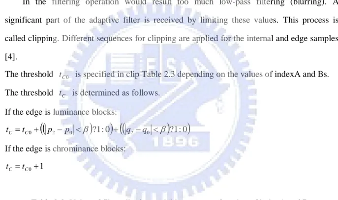
(28)  0  Clip3 tC , tC , q0  p0   2   p1  q1   4  3. tC  tC 0  1. (2.17). p0'  p0   0. q0'  q0   0 Otherwise. p1  p1 p2'  p2 p3'  p3. q1'  q1. q2'  q2. q3'  q3. Clipping Operation In the filtering operation would result too much low-pass filtering (blurring). A significant part of the adaptive filter is received by limiting these values. This process is called clipping. Different sequences for clipping are applied for the internal and edge samples [4]. The threshold t C 0 is specified in clip Table 2.3 depending on the values of indexA and Bs. The threshold t C is determined as follows. If the edge is luminance blocks: tC  tC 0   p2  p0   ?1 : 0   q2  q0   ?1 : 0. If the edge is chrominance blocks: tC  tC 0  1. Table 2.3: Value of filter clipping variable t C 0 as a function of indexA and Bs. index A 0. 1. 2. 3. 4. 5. 6. 7. 8. 9. 10. 11. 12. 13. 14. 15. 16. 17. 18. 19. 20. 21. 22. 23. 24. 25. Bs=1. 0. 0. 0. 0. 0. 0. 0. 0. 0. 0. 0. 0. 0. 0. 0. 0. 0. 0. 0. 0. 0. 0. 0. 1. 1. 1. Bs=2. 0. 0. 0. 0. 0. 0. 0. 0. 0. 0. 0. 0. 0. 0. 0. 0. 0. 0. 0. 0. 0. 1. 1. 1. 1. 1. Bs=3. 0. 0. 0. 0. 0. 0. 0. 0. 0. 0. 0. 0. 0. 0. 0. 0. 0. 1. 1. 1. 1. 1. 1. 1. 1. 1. 18.

(29) index A 26. 27. 28. 29. 30. 31. 32. 33. 34. 35. 36. 37. 38. 39. 40. 41. 42. 43. 44. 45. 46. 47. 48. 49. 50. 51. Bs=1. 1. 1. 1. 1. 1. 1. 1. 2. 2. 2. 2. 3. 3. 3. 4. 4. 4. 5. 6. 6. 7. 8. 9. 10. 11. 13. Bs=2. 1. 1. 1. 1. 1. 2. 2. 2. 2. 3. 3. 3. 4. 4. 5. 5. 6. 7. 8. 8. 10. 11. 12. 13. 15. 17. Bs=3. 1. 2. 2. 2. 2. 3. 3. 3. 4. 4. 4. 5. 6. 6. 7. 8. 9. 10. 11. 13. 14. 16. 18. 20. 23. 25. 2.4.2 Stronger mode : ( Bs=4 ) For luminance blocks: If p 2  p0   and p0  q0    2  2 The filtering unit needs to read 6 samples (p3, p2, p1, p0, q0, and q1) and updates 3 samples (p2, p1 and p0). If q2  q0   and p0  q0    2  2 The filtering unit needs to read 6 samples (q3, q2, q1, q0, p0, and p1) and updates 3 samples (q2, q1 and q0).. Left 4*1 samples. right 4*1 samples. p3 p2 p1 p0 q0 q1 q2 q3 edge Update sample Read sample. Figure 2.13: Stronger mode operations for luminance block. For chrominance blocks: The filtering unit needs to read 4 samples (p1, p0, q0, and q1) and updates 2 samples (p0 and q0). 19.

(30) Left 4*1 samples. right 4*1 samples. p3 p2 p1 p0 q0 q1 q2 q3 edge Update sample Read sample. Figure 2.14: Stronger mode operations for chrominance block. Filtering for edges with Bs equal to 4 When all of the following conditions hold: p0  q0    2  2 p 2  p0   q 2  q0  . For luminance blocks: The variables p0' , p1' , p2' , p3' , q0' , q1' , q2' , q3' are derived by. p0'   p2  2  p1  2  p0  2  q0  q1  4  3. (2.18). p1'   p2  p1  p0  q0  2  2. (2.19). p2'  2  p3  3  p2  p1  p0  q0  4  3. (2.20). q0'   p1  2  p0  2  q0  2  q1  q2  4  3. (2.21). q1'   p0  q0  q1  q2  2  2. (2.22). q2'  2  q3  3  q2  q1  q0  p0  4  3. (2.23). q3'  q3. p3'  p3. For chrominance blocks: The condition in equation does not hold The variables p0' , p1' , p2' , p3' , q0' , q1' , q2' , q3' are derived by. p0'  2  p1  p0  q1  2  2. (2.24). q0'  2  q1  q0  p1  2  2 p1'  p1. p2'  p2 p3'  p3. (2.25) q1'  q1. q2'  q2 20. q3'  q3.

(31) Input 8 pixels ( p3, p2, p1, p0, q0, q1, q2, q3 ), Bs, α and β. Bs  0 p0  q0  . p1  p 0  . no. q1  q 0  . yes. Chrominance block. Is luminance block? no yes. Bs=1~3 Bs level selection. Bs level selection. Bs=4. Bs=1~3 Bs=4. p 2  p0  . Update pixels p0 and q0. p0'  2 p1  p0  q1  2  2. p0  q0    2  2. no. q 0'  2q1  q 0  p1  2  2. p 2  p0  . q 2  q0  . no. q 2  q0   yes. Update pixels p0, p1, p2 q0, q1, q2 Remain unchanged pixels p3 and q3. Update pixels p0 and q0 p0'  p0   0. yes. Update pixels p0 and q0 Remain unchanged pixels p1, p2, p3 q1, q2, q3. Update pixels p0, p1 q0, q1 Remain unchanged pixels p2, p3 q2, q3. q0'  q0   0. Update pixels p0 and q0 Remain unchanged pixels p1, p2, p3 q1, q2, q3. output. Figure 2.15: Flow chart of filtering process 21.

(32) 2.5. Related Work In H.264/AVC standard, the de-blocking filter processing order is that, the vertical edges. are filtered first, from left to right, and then horizontal edges are filtered, from top to bottom.. The filtering process is performed on the boundary between two 4×4 pixel blocks. A macro-block contains one luma block and two chroma blocks. The luma block have sixteen 4 ×4 pixel blocks, the chroma block have four 4×4 pixel blocks. The filter processing requests eight the top neighbor 4×4 pixel blocks and eight the left neighbor 4×4 pixel blocks. Therefore a macro-block filter processing altogether need 40 4×4 pixel blocks.. The de-blocking filter uses one block as unit to process all macro-blocks. Therefore filter ordering according to this criterion, the 4×4 sub-block edge, left edge is filtered first, right edge is filtered second, come again the top edge is filtered third, and lower edge is the last one. Each numeral is an edge of two adjacent 4×4 sub-blocks that equal to the filter unit processing four times.. 22.

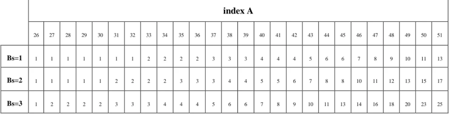
(33) 2.5.1 Basic Processing Order In [9], the basic processing order does not make use of data dependence between neighboring 4×4 pixel blocks as shown in figure 2.16. The example, the filtering operation is started with vertical edge 1, initially block (L1) and block (B0) are sent to the filter from internal memory using its two ports. After filtering of vertical edge 1, both the partially filtered block (L1) and block (B0) are stored into the internal memory. By this analogy, if we filter the vertical edge 5 in succession according to the basic filtering order. We have to load block (B0) and block (B1) from the internal memory, after filtering of vertical edge 5 stored the block (B0) and block (B1) back to the internal memory. The block (B0) is loaded and stored each two times. Thus it can be seen, the basic processing order does not make use of data dependence between neighboring 4×4 pixel blocks.. Supposition the memory system is 32-bit data bus, the basic processing order for a macro-block needs (4×2×2×16+(4×2×2×4)×2)=384 times of memory read and 384 times of memory write. The number of total memory access is 768 times.. U. T5. T6. 41. 42. L5 17 B16 19 B17. Y. T1. T2. T3. T4. 25. 26. 27. 28. 43. 44. L6 18 B18 20 B19 L1. 1. B0. L2. 2. B4. 5. B1. 6. B5 10 B6 14 B7. 29. 30. 33 B8. 34. B2 13 B3 31. 35. 32. 36. L3. 3. L4. 4 B12 8 B13 12 B14 16 B15. 37. 7. 9. B9 11 B10 15 B11 38. 39. 40. luma. V. T7. T8. 45. 46. L7 21 B20 23 B21 47. chroma. Figure 2.16: Basic processing order 23. 48. L8 22 B22 24 B23.

(34) 2.5.2 Advanced Processing Order In the figure 2.17 is shown the advanced filter processing order. It makes use of one-dimensional data dependence [9]. The example, the filtering operation is started with vertical edge 1, initially block (L1) and block (B0) are sent to the filter from internal memory using its two ports. After filtering of vertical edge 1, the partially filtered block (L1) is stored into the internal memory but the block (B0) is buffered in the de-blocking filter unit for next stage filtering. By this analogy, if we filter the vertical edge 2 in succession according to the filtering order. We have to load block (B1) from the internal memory and the block (B0) is buffered in the de-blocking filter unit. In this way, all the 4×4 pixel blocks in horizontal filtering and in vertical filtering can reduced to half access times for internal memory.. Supposition the memory system is 32-bit data bus, the advanced filter processing order for a macro-block needs (384-16×4×2)=256 times of memory read and 256 times of memory write. The number of total memory access is 512 times.. U. T5. T6. 41. 43. L5 17 B16 18 B17. Y. T1. T2. T3. T4. 25. 29. 33. 37. 42. 44. L6 19 B18 20 B19 L1. 1. B0. 2. 26 L2. 5. B4 27. L3. 9. B1. 3. 30 6. B5 31. B2. 4. 34 7. B6 35. B3 38. 8. B7 39. B8 10 B9 11 B10 12 B11 28. 32. 36. 40. V. T7. T8. 45. 47. L7 21 B20 22 B21 46. 48. L4 13 B12 14 B13 15 B14 16 B15. L8 23 B22 24 B23. luma. chroma. Figure 2.17: Advanced processing order. 24.

(35) 2.5.3 2-D Processing Order In the figure 2.18 is shown the 2-D filter processing order. The filter order conforms to the de-blocking filter processing standard. It is performed alternately to the horizontal filtering and the vertical filtering [10]. For example, the filtering operation is started with vertical edge 1, the block (L1) and block (B0) were sent to the filter from internal memory using its two ports. After filtering of vertical edge 1, the block (L1) is stored back to the internal memory, the other block (B0) is buffered in the de-blocking filter unit for next stage filtering. After the last filtering, the vertical edge 2, the block (B0) is sent to the transpose buffer wait for the horizontal edge 3 filtering, the block (B1) is buffered in the de-blocking filter unit for next stage vertical edge 4 filtering.. Supposition the memory system is 32-bit data bus, the 2-D filter processing order for a macro-block needs (4×12+4×12×2+(4×6+4×2×2)×2)=224 times of memory read and 224 times of memory write. The number of total memory access is 448 times.. U. T5. T6. 35. 36. L5 33 B16 34 B17. Y. T1. T2. T3. T4. 3. 5. 7. 8. 39. 40. L6 37 B18 38 B19 L1. 1. B0 11. L2. 9. 2. B1 13. 4. B2 15. 6. B3 16. B4 10 B5 12 B6 14 B7 19. 21. 23. 24. L3 17 B8 18 B9 20 B10 22 B11 27. 29. 31. 32. V. T7. T8. 43. 44. L7 41 B20 42 B21 47. 48. L4 25 B12 26 B13 28 B14 30 B15. L8 45 B22 46 B23. luma. chroma. Figure 2.18: 2-D processing order. 25.

(36) 2.5.4 2-D Simultaneous Processing Order In the figure 2.19 is shown the 2-D simultaneous filter processing order. It is performed alternately and simultaneous processing order of the horizontal filtering of vertical edge and the vertical filtering of horizontal edge [5]. The figure shows, it was used by one the horizontal filter unit and one the vertical filter unit to simultaneous processing order. This method goal is in order to reduce when clock cycles quantity. Supposition the memory system is dual port RAMs and the data bus is 32-bit.. For example, the filtering operation is started with vertical edge 1, the block (L1) and block (B0) are sent to the filter from internal memory using its two ports. After filtering of vertical edge 1, the block (L1) is stored back to the internal memory, the other block (B0) is buffered in the de-blocking filter unit for next stage filtering. After the last filtering, the vertical edge 2, the block (B0) is sent to the transpose buffer wait for the horizontal edge 3 filtering, the block (B1) is buffered in the de-blocking filter unit for next stage vertical edge 3 filtering.. U. T5. T6. 19. 20. L5 17 B16 18 B17. Y. T1. T2. T3. T4. 3. 4. 5. 6. 21. 22. L6 19 B18 20 B19 L1. 1. B0. L2. 5. B4. 2. B1. 6. B5. 7. 11 L3. 9. 3. B2. 7. B6. 8. 12. 4. B3. 8. B7. 9. 13. 10. 14. B8 10 B9 11 B10 12 B11 15. 16. 17. 18. V. T7. T8. 23. 24. L7 21 B20 22 B21 25. 26. L4 13 B12 14 B13 15 B14 16 B15. L8 23 B22 24 B23. luma. chroma. Figure 2.19: 2-D simultaneous processing order 26.

(37) 2.5.5 Summary related work Table 2.4: comparison of above proposed architecture. Basic. Advanced. 2-D Simultaneous. [9]. [9]. [5]. Cycles/MB. 712. 760. 460. Filtering Cycles/MB. 392. 440. 140. External memory access cycles. 320. 320. 320. Working frequency. 100 MHz. 100 MHz. 100 MHz. Edge Filters. 1. 1. 2. 4× 4 array. 2. 2. 3. 4× 4 FIF0. 0. 0. 9. Techno logy (μ m). 0.25. 0.25. 0.13. Gate count. 18.91K. 18.91K. 35.99K. Method. Memory architecture. One read and one One read and one Two read and two write SRAM write SRAM write SRAM. SRAM requirements for pixels (bit s). 88× 32 72× 32. 160× 32. 88× 32 72× 32. All gate counts don’t include SRAM. The basic [9] and 2-D Simultaneous [5] are use two SRAM modules and interleaved memory organization to store the pixel data of a macro-block for efficient access of pixels in different blocks of the macro-block.. 27.

(38) Chapter 3 Proposed architecture of de-blocking filter In this chapter, we propose our architecture. In section 3.1 we present the main parts of the architecture for the de-blocking filter. In section 3.2 we show the proposed filtering order and how it reduces internal memory size. In section 3.3 we describe the internal memory organization. In section 3.4 we describe the data buffer and transpose buffer about how they work. In section 3.5 we present our control unit about how it works.. 3.1. Overview of the Proposed Architecture Figure 3.1 shows the main parts of the architecture for the de-blocking filter. It includes. the external memory, internal SRAM, filter unit, data buffer, transpose buffer and control unit. The following comes to introduce these constructions individually the basic function.. Coding Info.. Nonfiltered pixels. Internal SRAM External memory. Control Unit. Filter unit. Filtered pixels. Data buffer Bus interface. Transpose buffer. Figure 3.1: System architecture of the de-blocking filter 28.

(39) External Memory: The purpose of external memory is stored the frame data that processed by decoder. The external memory provides the unfiltered data to the de-blocking filter and according to the filter order. When current frame was processed, the next frame is going to send to the external memory. The reconstruction frame is provided to the motion compensation use.. Internal SRAM: A macro-block data is loaded to the internal SRAM from the external memory. Generally speaking, the internal SRAM size is 32-bit×160 because consisted of a 16×16 luma block, two 8×8 chroma block, and sixteen 4×4 neighbor block. When current macro-block was processed, the next macro-block is going to send to the internal SRAM.. Filter unit: The edge filter unit is a parallel-in parallel-out filter, the input end is two 32-bit data bus and output end is two 32-bit data bus. Its interior has the different operation pattern that may choose because of the different parameter.. Data Buffer: In the basic processing order does not make use of data dependence between neighboring 4×4 pixel blocks, therefore does not need data buffer. But after the processing order makes use of the data dependence, therefore needs data buffer to reduce the memory the access number of times.. Transpose Buffer: The transpose buffer function is uses in the vertical filtering across horizontal edges. When the horizontal filtering across vertical edges of the data processes places in the transpose buffer to make the transformation afterwards.. 29.

(40) Control Unit: The control unit of de-blocking filter module is to control the signals such as Bs, C0, α, β the information and so on. Moreover a function is controls the data the input-output.. In our architecture design, first we will find a new filter processing order. By the new filter processing characteristic we may obtain the data dependence and data reuse strong point. Because of these merit, we may reduce the number of memory references, decrease the required memory size and using fewer the register amounts, and speed up the whole filtering process. Afterwards chapter, we will be able individual to introduce each construction. Understanding the whole architecture, how realization and operation.. 3.2 Filtering Order 3.2.1 De-blocking filter order of the 4×4 sub-block edge The de-blocking filter uses one 4×4 pixels block as unit to process all macro-blocks. The de-blocking filter in H.264/AVC is performed in the vertical edge first, and then the horizontal edge. Therefore filter ordering according to this criterion, the 4×4 sub-block edge, left edge is filtered first, right edge is filtered second, come again the top edge is filtered third, and lower edge is the last one as shown in figure 3.2. macro-block. 3 1. 2 4. Figure 3.2: De-blocking filter order of the 4×4 sub-block edge 30.

(41) 3.2.2 Proposed edge filtering order Our filtering order is illustrated in figure 3.3. It is a macro-block filtering to need the data, the blocks B0 to B23 are the current macro-block, the blocks T1 to T8 are the top neighbor block that were provided the vertical filtering across horizontal edges to use, the blocks L1 to L8 are the left neighbor block that were provided the horizontal filtering across vertical edges to use. In our proposed de-blocking filter architecture is to use two edge filter units, the goal is reduce the filter processing cycles, which support real-time de-blocking of HDTV with higher resolution.. U. T5. T6. 19. 19. L5 17 B16 18 B17. Y. T1. T2. T3. T4. 4. 4. 7. 7. 20. 20. L6 17 B18 18 B19 L1. 1. B0. 2. 5 L2. 1. B4 12. L3. 9. 3. 5 2. B5 12. B2. 6. B3. 8 3. B6 15. 8 6. B7 15. B8 10 B9 11 B10 14 B11 13. L4. B1. 13. 16. 16. 9 B12 10 B13 11 B14 14 B15. luma. V. T7. T8. 23. 23. L7 21 B20 22 B21 24. 24. L8 21 B22 22 B23. chroma. Figure 3.3: Proposed filtering order. The figure 3.3 shows the two edge filter units are simultaneous processing and we indicated the horizontal filtering across vertical edges by the red circle, the vertical filtering across horizontal edges by green circle. In circle numeral is expressed of filter order. Each numeral is an edge of two adjacent blocks that equal to the filter unit processing four times.. 31.

(42) 3.2.3 Divide the luma block According to the filter order, we may divide into luma block two parts. The processing order 1 to 8 and 9 to 16 are same filtering order. As shown in Figure 3.4.. processing order (1, 9). processing order(2, 10). processing order(3, 11). processing order (4, 12). processing order (5, 13). processing order (6, 14). processing order(7, 15). processing order (8, 16). Figure 3.4: Luma block of the filtering order About the luma block may open the solution after ours filter order to become two parts, as shown in Figure 3.5. After luma block upper half was filtered, the blocks B4, B5, B6, and B7 were passed through the transpose buffer to make the transformation then stored to the internal SRAM. When the luma block lower half was filtered, the blocks B4 to B7 may use directly, but does not have again to pass through the transformation.. Y. T1. T2. T3. T4. T1. T2. T3. T4. L1. B0. B1. B2. B3. L1. B0. B1. B2. B3. L2. B4. B5. B6. B7. L2. B4. B5. B6. B7. L3. B8. B9. B10. B11. L4. B12. B13. B14. B15. =. luma. + B4. B5. B6. B7. L3. B8. B9. B10. B11. L4. B12. B13. B14. B15. Figure 3.5: Luma block break down upper and the lower two parts 32.

(43) Because of ours filtering order can reduce the size of the internal SRAM, decreases the transpose buffer use quantity, improves the throughput of filtering operations, and the amount of reduction of the external memory accesses.. 3.3 Parallel Memory Unit Because we simultaneously use two edge filter units to make the operation, therefore these input ends of two edge filter units also must simultaneously obtain the pixel data. So we use two 32-bits×48 dual ports SRAM to store the pixels data needed. As shown in Figure 3.6, we divide the pixels data within one macro-block into the form of the interlocking type, have corresponding internal SRAM individually pixels data its.. We use their purposes of the way of the interlocking type to be to take place for the phenomenon of preventing the memory from conflicting. The pixels data needed can do parallel access at we are making the horizontal filtering across vertical edges and making the vertical filtering across horizontal edges.. 32 bits 32 bits. Y. 32 bits. T1. L1. B0. 20 L2 words. B4. L3. B8. 32 bits. T2. 32 bits. T3. 32 bits. U. T4. L5. 32 bits. T5. 32 bits. T6. 12 B16 B17 words. B1. B2. B3. L6 B18 B19. B5. B6. B7. V. B9 B10 B11. 48 (words). L7. T7. T8. 12 B20 B21 words. 32 bits. 32 bits. L1. L2. B4. B0. B1. B5. B6. B2. B3. B7. T1' T3' L5. 48 (words). T2' T4' L6. B18. B16. B17. B19. T5'. T6'. L4 B12 B13 B14 B15. L8 B22 B23. T7'. T8'. luma. chroma. 48´32 SRAM 0. 48´32 SRAM 1. Figure 3.6: Memory mapping of 4×4 blocks. 33.

(44) As shown in Figure 3.6, the T1', T2', T3', T4', T5', T6', T7', and T8' are the 4×4 block pixel data got after the transpose buffer to make the transformation afterwards to putting after dealing with by the horizontal filtering across vertical edges first. So they can be used directly that the blocks T1' to T8' needn't to make the transformation afterwards and put when doing the vertical filtering across horizontal edges. The interleaving nature of data organization allows for simultaneous writing and reading of data to and from the internal SRAM.. 3.4 Data Buffer ＆ Transpose Buffer Data buffer As shown in Figure 3.7, the 4×4 block B0 have sixteen pixel (b00~b33), each pixel can be stored 8-bits. Input and output of the de-blocking filter regard four pixels (32-bits) as a unit. So need to spend four cycles (one block cycle) to finish to one edge of the 4×4 block.. 1 L1 1 B0 2 B1. 2. Filtering order. b00 b01 b02 b03 b10 b11 b12 b13 b20 b21 b22 b23 b30 b31 b32 b33. 4*4 block B0 16*16 macro-block. Figure 3.7: for example a 4×4 block. As shown in Figure 3.7 and 3.8, the 4×4 blocks L1, B0, and B1 are the neighboring three blocks. Now we must first de-blocking filter block L1 and the block B0 middle vertical edge then again make between block B0 and the block B1 the vertical edge. Therefore we input L1 to the filter unit of p (p0~p3) input end, input B0 to the filter unit of q (q0~q3) input end,. 34.

(45) causes both to make the filtering order 1 the movement. After the filtering order 1 completes, processing from now on pixels of the block B0 will be able to deposit in data buffer in order to next the filtering order 2 use. Therefore because of the data buffer use, we may reduce from internal SRAM read data number of times.. 4 pixel (32-bit). 4 pixel (32-bit). p3 p2 p1 p0. q0 q1 q2 q3. Filter unit. b30' b31' b32' b33' b20' b21' b22' b23' b10' b11' b12' b13'. Output to transpose buffer or internal SRAM. b00' b01' b02' b03'. Data buffer p3 p2 p1 p0 Figure 3.8: Data buffer operation. Transpose Buffer In our proposed de-blocking filter architecture to use two 32-bits×8 transpose registers to transpose the pixels which obtains by way of the horizontal filtering across vertical edges. As shown in Figure 3.9 this is group of two 32-bits×4 transpose registers. Every small square represents 1 pixel (8-bits) register. The solid line of arrows expresses the input data path while the dotted line of arrows expresses the output data path. And the data bus input and outputted are all 4 pixels (32-bits). For example, it needs to spend four cycles to store the sixteen pixels to transpose a 4×4 block. When processing the vertical filtering across horizontal edges, we can output the pixels data that we need with the selector.. 35.

(46) 4 pixels (32-bits). 4 pixels (32-bits). Figure 3.9: Transpose buffer operation. 3.5. Control Unit Figure 3.10 shows the overall architecture of our proposed de-blocking filter and the data. bus is all 32-bits. It includes the internal SRAM size is 32-bit×96, two parallel-in parallel-out filter unit, two data buffer of 32-bits×4 FIFO register, four transpose register and a control unit. Some of control unit that is very important component, it is to control the signals such as Bs, C0, α, β the information and so on. Moreover a function is controls the data the input-output. So we explain next how the controller controls the flow of pixel data with the part of upper part of Luma block. We make necessary pixels data from external memory load to internal SRAM at first.. 36.

(47) FIFO. Filter unit Filter unit. Internal SRAM. FIFO. Transpose buffer. Figure 3.10: Overall architecture of our proposed de-blocking filter. Step 1: block cycle 1 (clock cycle 1~4). At first, we load L1 and L2 of the left neighbor block from the internal SRAM then input them in two data buffer separately, use for horizontal filtering on vertical edge 1 after offering. L2³. FIFO. L1³. FIFO. L2³ B0 B5 B2 B7 T2³ T4³ L6³ B16 B19 T6³ T8³. Filter unit. L1³ B4 B1 B6 B3 T1³ T3³ L5³ B18 B17 T5³ T7³. Filter unit. to. As shown in Figure 3.11.. Figure 3.11: The data path of storing block of L1 and L2 into data buffer 37.

(48) Step 2: block cycle 2 (clock cycle 5~8) Figure 3.12 shows the horizontal filtering on vertical edge 1 treating processes. Therefore we load the block B0 and B4 from internal SRAM at the same time, lets two filter units make the use. After horizontal filtering on vertical edge 1 completes that the blocks L1 and L2 are stored to internal SRAM, the blocks B0 and B4 are stored to the data buffer,. B4¹. FIFO. B0¹. FIFO. L2* B0 B5 B2 B7 T2³ T4³ L6³ B16 B19 T6³ T8³. Filter unit. L1* B4 B1 B6 B3 T1³ T3³ L5³ B18 B17 T5³ T7³. Filter unit. waiting next filtering order uses.. Figure 3.12: Horizontal filtering on vertical edge 1. Step 3: block cycle 3 (clock cycle 9~12) Figure 3.13 shows the horizontal filtering on vertical edge 2 treating processes. Therefore we load the block B1 and B5 from internal SRAM at the same time to give two filter units uses separately. After the horizontal filtering on vertical edge 2 processing completes, the blocks B1 and B5 are stored up to the data buffer, the blocks B0 and B4 are transmitted the transpose buffer to make the transformation (B0 and B4) that to wait for vertical filtering.. 38.

(49) B5¹. B1¹. FIFO. Filter unit. B4². FIFO. L2* B0 B5 B2 B7 T2³ T4³ L6³ B16 B19 T6³ T8³. Filter unit. L1* B4 B1 B6 B3 T1³ T3³ L5³ B18 B17 T5³ T7³. B0². Figure 3.13: Horizontal filtering on vertical edge 2 Step 4: block cycle 4 (clock cycle 13~16) Figure 3.14 shows the horizontal filtering on vertical edge 3 treating processes. This step is the same as process of step 3. After the horizontal filtering on vertical edge 3 processing completes, the blocks B1 and B5 are transmitted the transpose buffer to make the transformation (B1 and B5) that to wait for vertical filtering. The thing that should look out is that the blocks B0 and B1 can't be placed on the same group of the transpose buffers,. B2¹. FIFO. B6¹. B1² B4². FIFO. L2* B0 B5 B2 B7 T2³ T4³ L6³ B16 B19 T6³ T8³. Filter unit. L1* B4 B1 B6 B3 T1³ T3³ L5³ B18 B17 T5³ T7³. Filter unit. otherwise will cause the conflict of the data. So the blocks B4 and B5 are the same situation.. B5² B0². Figure 3.14: Horizontal filtering on vertical edge 3 39.

(50) Step 5: block cycle 5 (clock cycle 17~20) As shown in Figure 3.15. We load T1 and T2 of the top neighbor block from the internal SRAM then input them in two data buffer separately, use for vertical filtering on horizontal edge 4 after offering to. Does not act in this stage of two filter unit, therefore the blocks B2. T1³. FIFO. T2³. B1² B4². FIFO. L2* B0 B5 B2¹ B7 T2³ T4³ L6³ B16 B19 T6³ T8³. Filter unit. L1* B4 B1 B6¹ B3 T1³ T3³ L5³ B18 B17 T5³ T7³. Filter unit. and B6 pixels data has not been changed on is stored directly the internal SRAM.. B5² B0². Figure 3.15: The data path of storing block of T1 and T2 into data buffer. Step 6: block cycle 6 (clock cycle 21~24) Figure 3.16 shows the vertical filtering on horizontal edge 4 treating processes. Therefore we load the block B0 and B1 from transpose buffer at the same time, lets two filter units make the vertical filtering. After the vertical filtering on horizontal edge 4 processing completes, the blocks T1 and T2 are stored to transpose buffer make the transformation (T1 and T2), after in order to store the internal SRAM.. 40.

(51) B1³. B0³. FIFO. Filter unit. T2* B4². FIFO. L2* B0 B5 B2¹ B7 T2³ T4³ L6³ B16 B19 T6³ T8³. Filter unit. L1* B4 B1 B6¹ B3 T1³ T3³ L5³ B18 B17 T5³ T7³. B5² T1*. Figure 3.16: Vertical filtering on horizontal edge 4. Step 7: block cycle 7 (clock cycle 25~28) Figure 3.17 shows the vertical filtering on horizontal edge 5 treating processes. This step is the same as process of step 6. After the vertical filtering on horizontal edge 5 processing completes, the blocks B0 and B1 are stored to transpose buffer make the transformation (B0. B4³. FIFO. B5³. T2* B0*. FIFO. L2* B0 B5 B2¹ B7 T2³ T4³ L6³ B16 B19 T6³ T8³. Filter unit. L1* B4 B1 B6¹ B3 T1³ T3³ L5³ B18 B17 T5³ T7³. Filter unit. and B1) that to wait for storing the internal SRAM.. B1* T1*. Figure 3.17: Vertical filtering on horizontal edge 5 41.

(52) Step 8: block cycle 8 (clock cycle 29~32) This stage of two filter unit is not act. We load the blocks B2 and B6 from the internal SRAM then input them in two data buffer separately, use for the horizontal filtering on vertical edge 6 after offering to. The blocks T1 and T2 are stored to the internal SRAM, the blocks B4 and B5 are stored to transpose buffer but not make the transformation as shown in. B2¹. FIFO. B6¹. B5³ B0*. FIFO. L2* B0 B5 B2¹ B7 T2* T4³ L6³ B16 B19 T6³ T8³. Filter unit. L1* B4 B1 B6¹ B3 T1* T3³ L5³ B18 B17 T5³ T7³. Filter unit. figure 3.18.. B1* B4³. Figure 3.18: The data path of storing block of B2 and B6 into data buffer. Step 9: block cycle 9 (clock cycle 33~36) Figure 3.19 shows the horizontal filtering on vertical edge 6 treating processes. Therefore we load the block B3 and B7 from internal SRAM at the same time to give two filter units uses separately. After the horizontal filtering on vertical edge 6 processing completes, the blocks B3 and B7 are stored up to the data buffer, the blocks B2 and B6 are transmitted the transpose buffer to make the transformation (B2 and B6) that to wait for vertical filtering and the blocks B0 and B1 are stored to the internal SRAM simultaneously.. 42.

(53) B7¹. B3¹. FIFO. Filter unit. B5³ B6². FIFO. L2* B0* B5 B2¹ B7 T2* T4³ L6³ B16 B19 T6³ T8³. Filter unit. L1* B4 B1* B6¹ B3 T1* T3³ L5³ B18 B17 T5³ T7³. B2² B4³. Figure 3.19: Horizontal filtering on vertical edge 6 Step 10: block cycle 10 (clock cycle 37~40) As shown in Figure 3.20. We load T3 and T4 of the top neighbor block from the internal SRAM then input them in two data buffer separately, use for the vertical filtering on horizontal edge 7 after offering to. Does not act in this stage of two filter units, therefore the blocks B3 and B7 pixels data have not been changed and to store directly the transpose buffer.. T3³. FIFO. T4³. B3¹ B6². FIFO. L2* B0* B5³ B2¹ B7 T2* T4³ L6³ B16 B19 T6³ T8³. Filter unit. L1* B4³ B1* B6¹ B3 T1* T3³ L5³ B18 B17 T5³ T7³. Filter unit. And the blocks B4 and B5 are stored to the internal SRAM simultaneously.. B2² B7¹. Figure 3.20: The data path of storing block of T3 and T4 into data buffer 43.

(54) Step 11: block cycle 11 (clock cycle 41~44) Figure 3.21 shows the vertical filtering on horizontal edge 7 treating processes. Therefore we load the block B2 and B3 from transpose buffer at the same time, lets two filter units make the vertical filtering. After the vertical filtering on horizontal edge 7 processing completes, the blocks T3 and T4 are stored to transpose buffer make the transformation (T3. B2³. FIFO. B3². T4* B6². FIFO. L2* B0* B5³ B2¹ B7 T2* T4³ L6³ B16 B19 T6³ T8³. Filter unit. L1* B4³ B1* B6¹ B3 T1* T3³ L5³ B18 B17 T5³ T7³. Filter unit. and T4), after in order to store the internal SRAM.. T3* B7¹. Figure 3.21: vertical filtering on horizontal edge 7. Step 12: block cycle 12 (clock cycle 45~48) Figure 3.22 shows the vertical filtering on horizontal edge 8 treating processes. This step is the same as process of step 11. After the vertical filtering on horizontal edge 8 processing completes, the blocks B2 and B3 are stored to transpose buffer make the transformation (B2 and B3) that to wait for storing the internal SRAM.. 44.