適用於行動裝置之高效率節能機制

國

立

交

通

大

學

資訊科學與工程研究所

博

士

論

文

適用於行動裝置之高效率節能機制

Efficient Energy Saving Techniques for Mobile Devices

研 究 生：施宏政

指導教授：王國禎 教授

適用於行動裝置之高效率節能機制

Efficient Energy Saving Techniques for Mobile Devices

研

究 生：施宏政 Student：Hung-Cheng Shih

指導教授：王國禎

Advisor：Kuochen Wang

國

立 交 通 大 學

資

訊 科 學 與 工 程 研 究 所

博

士 論 文

A Dissertation

Submitted to Institute of Computer Science and Engineering Department of Computer Science

National Chiao Tung University in partial Fulfillment of the Requirements

for the Degree of Doctor of Philosophy

in

Computer Science July 2012

Hsinchu, Taiwan, Republic of China

適用於行動裝置之高效率節能機制

學生：施宏政 指導教授：王國禎博士

國立交通大學資訊科學與工程研究所

摘 要

我們提出一個高能源效率，具有適應性之動態能源管理演算法。為了

能夠適應具爆發性與自我相似之需求到達模式及具多重閒置狀態之裝置，

我們先分別求得需求爆發

(ON)時期和無需求(OFF)時期的平均裝置閒置時

間。接著，為了達到更好的節能效率，我們利用需求爆發時期的平均裝置

閒置時間來調整將裝置切入低耗能狀態前的等待時間。實驗結果顯示，針

對行動式硬碟，我們所提出的演算法之平均能源消耗量低於動態等待時間

調 整

(Adaptive Timeout)，機器學習(Machine Learning)，預測閒置時間

(Predictive)，固定等待時間調整(Static Timeout)，及隨機狀態切換(Stochastic)

等演算法。另外，本演算法之平均裝置回應時間也低於標準行動式硬碟的

規範。至於無線網路裝置，其平均能源消耗量也接近先知型

(Oracle，理論

學習，固定等待時間，及隨機狀態切換等演算法。但是，本演算法之平均

封包傳輸延遲優於動態等待時間調整及預測閒置時間等演算法。所以，本

演算法提供了較佳的平均能源消耗量與平均裝置回應時間

(或平均封包傳輸

延遲

)，而使得本演算法非常適合用於延長具有行動式硬碟與無線網路裝置

之行動裝置的電池使用時間。

關鍵詞：硬碟，行動裝置，能源管理，自我相似，無線網路介面卡

Efficient Energy Saving Techniques for

Mobile Devices

Student：Hung-Cheng Shih Advisor：Dr. Kuochen Wang

Institute of Computer Science and Engineering National Chiao Tung University

Abstract

We propose a power efficient adaptive hybrid dynamic power management (AH-DPM) algorithm. To adapt to bursty request arrival patterns with self-similarity and a service provider (SP, i.e., hard disk or WLAN NIC, in this dissertation) with multiple inactive states, the proposed AH-DPM first derives the average idle time of the SP in the bursty (ON) period and non-bursty (OFF) period separately. Then, to achieve better power saving, we use the average idle time in the ON period to adjust the timeout value more precisely and use the average idle time in the OFF period to decide which inactive state the SP should be switched to. Experimental results based on real traces show that, for the hard disk, the average power consumption of the proposed AH-DPM is better than that of the Adaptive Timeout (ATO), Machine Learning (ML), Predictive, Static Timeout (STO), and Stochastic algorithms. In addition, the average response time of the proposed AH-DPM algorithm is still lower than that specified in a typical hard disk specification. As to the WLAN NIC, experimental results show that the average power consumption of the proposed AH-DPM is comparable to that of the Oracle (theoretically optimal), ATO, and Predictive algorithms, and is better than that of

the proposed AH-DPM is better than that of ATO and Predictive algorithms. Therefore, by providing a better tradeoff between average power consumption and average response time (or average packet transmission delay), the proposed AH-DPM algorithm is very feasible for extending the battery lifetime of mobile devices that are equipped with hard disks and WLAN NICs.

Acknowledgements

Special thanks go to my dissertation advisor, Professor Kuochen Wang, for his intensive advice and instruction. Thanks also go to the dissertation oral exam committee members, Prof. Sy-Yen Kuo, Prof. Yu-Chee Tseng, Prof. Hsi-Lu Chao, Prof. Jang-Ping Sheu, Prof. Woei Lin, and Prof. Chu-Sing Yang, for their suggestions to this dissertation. Thanks to all the members in Mobile Computing and Broadband Networking Laboratory for their invaluable assistance and kind help both in the research and daily life during these years. The support of the National Science Council, Taiwan, under Grants NSC96-2628-E-009-140-MY3 and NSC99-2221-E-009-081-MY3 is greatly appreciated.

Finally, my family deserves special mention. This dissertation is dedicated to them for their continued love and support.

Contents

摘 要 ... i

Abstract ... iii

Acknowledgements ... v

Contents ... vi

List of Figures ... viii

List of Tables ... x

Chapter 1 Introduction ... 1

1.1 Overview of the DPM ... 2

1.2 Self-similarity characteristic of hard disk and WLAN NIC workloads ... 2

1.3 Motivation and main contributions of this work ... 5

Chapter 2 Related Work ... 6

2.1 Timeout-based algorithms ... 6

2.2 Predictive-based algorithms ... 7

2.3 Stochastic-based algorithms ... 10

2.4 Machine learning algorithms ... 13

3.1 The design of the proposed algorithm ... 17

3.2 The flowchart and pseudo codes of the proposed algorithm ... 20

Chapter 4 Experimental Results and Discussion ... 24

4.1 Experimental setup ... 24

4.2 Experimental results ... 30

4.3 Discussion ... 41

Chapter 5 Conclusions and Future Work ... 44

5.1 Concluding remarks ... 44 5.2 Future work ... 45 Bibliography ... 47 Vita... 50 Publication List ... 51 Journal Papers ... 51

Manuscripts in Prepartion for Submission to Journals ... 51

Conference Papers ... 51

Book Chapters ... 52

List of Figures

Fig. 1-1. An example of a component’s request arrival pattern, working pattern, and power

level transitions. ... 3

Fig. 2-1. The classification of existing DPM algorithms. ... 6

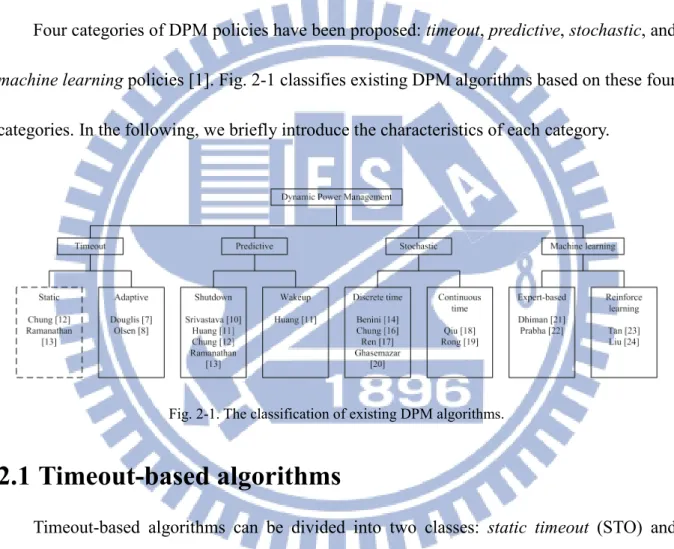
Fig. 2-2. Overall system architecture for the DPM [14]. ... 11

Fig. 3-1. The flowchart of the proposed AH-DPM algorithm. ... 22

Fig. 3-2. Inactive state decision algorithm. ... 22

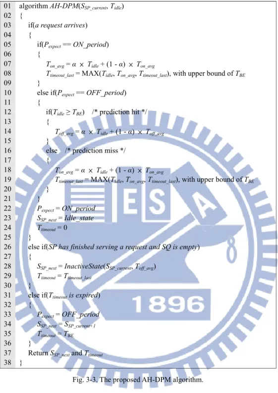
Fig. 3-3. The proposed AH-DPM algorithm. ... 23

Fig. 4-1. The state transition diagram of Hitachi Travelstar 5K100 hard disk. ... 28

Fig. 4-2. The state transition diagram of the WLAN NIC. ... 29

Fig. 4-3. Comparison of the average power consumption of the hard disk ... 31

Fig. 4-4. Comparisons of the average response time of the hard disk. ... 32

Fig. 4-5. Comparisons of the inactivation ratio of the hard disk. ... 32

Fig. 4-6. Comparison of the average power consumption of the hard disk in a week. ... 34

Fig. 4-7. The comparison of average response time of the hard disk in a week. ... 34

Fig. 4-8. The prediction miss rate of the hard disk in a week. ... 35

Fig. 4-10. Comparisons of average packet transmission delay of the WLAN NIC. ... 36

Fig. 4-11. Comparison of inactivation ratio of the WLAN NIC... 37

Fig. 4-12. Average power consumption of the WLAN NIC in a week. ... 38

Fig. 4-13. Average packet transmission delay of the WLAN NIC in a week. ... 39

Fig. 4-14. Prediction miss rate of the WLAN NIC in a week. ... 39

List of Tables

Table 2-1. A qualitative comparison of representative DPM algorithms. ... 15 Table 3-1. The parameters used in the proposed AH-DPM algorithm. ... 17 Table 4-1. State transition time and power consumption specifications of Hitachi Travelstar 5K100 hard disk [26]. ... 28 Table 4-2. Power consumption specification of Hitachi Travelstar 5K100 hard disk [26]. . 28 Table 4-3. Trace characteristics of hard disk requests. ... 29 Table 4-4. Power consumption specification of Intel PRO/Wireless 3945ABG WLAN NIC [29]. ... 29 Table 4-5. State transition time and power consumption of the WLAN NIC [29][30]. ... 29 Table 4-6. Trace characteristics of WLAN NIC traffic. ... 30

Chapter 1

Introduction

In recent years, mobile devices are getting more pervasive and popular due to a wider spread of wireless internet. Because mobile devices have the characteristic of mobility, their power sources must rely on battery power. Due to increasing demands of users on performance and functionality of mobile devices, the power consumption of these devices will enlarge. Battery lifetime in mobile devices can be prolonged in two ways: increasing battery capacity per unit weight and reducing power consumption with minimal performance loss [1]. Since the battery capacity per unit weight has only improved by a factor of two to four over the last 30 years while the computational power of digital ICs has increased by more than four orders of magnitude, reducing the power consumption of components in mobile devices become a vital issue. That is, in order to extend the battery lifetime, managing the power consumption of components in a mobile device is essential. Since not all components in a mobile device are active at the same time, we can switch some components to low power consumption states when they are idle for a certain period of time. The concept of switching between different states with different power consumption levels has been introduced to the design of components in mobile devices. With this capability, we can dynamically switch a

1.1 Overview of the DPM

Dynamic power management (DPM) is an effective approach for mobile devices to reduce power consumption without significantly degrading their performance. The DPM shuts down components when they are not being used and wakes them up when necessary [2]. With careful observation of components’ state transition patterns, the DPM can predict when an idle period will likely occur. The operating system (OS) in a DPM-enabled mobile device has a module called Power Manager (PM). The PM is responsible for monitoring all components in a mobile device and controlling the working state of each component [1]. The PM has several power management policies, possibly one policy for one component according to its working pattern. These policies are used by the PM to decide at what time and which state a component should be transferred to. It is important that power management policies have to be adaptive because arrival patterns of service requests are usually non-stationary [16]. If we confine a fixed power management policy to all possible working patterns, the effect of power management will not be good.

1.2 Self-similarity characteristic of hard disk and WLAN

NIC workloads

A self-similar stochastic process is a stochastic process that all statistical properties remain unchanged at various observation time scales. That is, the stochastic process “looks the same” if one zooms in time “in and out” in the process [3]. The observed shape of a self-similar stochastic process in a time scale of milliseconds would be still similar to that in a

time scale of seconds, hours, or even days. According to the studies of Xiang et al. [4] and Gomez et al. [5][6], both hard disk access patterns and WLAN NIC traffic are bursty and

self-similar. That is, the patterns of hard disk access and WLAN NIC traffic are always bursty

no matter how long we observe them. Bursty arrival patterns with self-similarity can be modeled by the ON-OFF model [5][6]. In ON (bursty) periods, the hard disk (WLAN NIC) idle time is short compared with that in OFF (non-bursty) periods. If we compare the hard disk (WLAN NIC) idle time with the break-even time, we can see that there will be periods that the hard disk (WLAN NIC) idle time are shorter than the break-even time. We define these periods as ON periods. The other periods with the hard disk (WLAN NIC) idle time longer than or equal to the break-even time are called OFF periods. In the OFF periods, the hard disk (or WLAN NIC) has to be switched to a low power consumption state in order to save power.

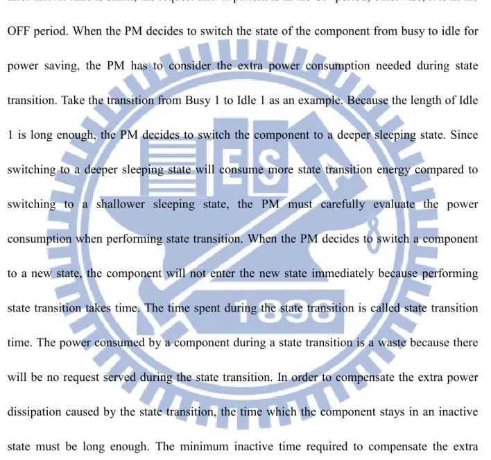
Fig. 1-1 is an example of a component’s request arrival pattern, working pattern, and power level transitions. Since the request arrival pattern is bursty, we can divide the request arrival pattern into two kinds of periods: ON period and OFF period. When the request inter-arrival time is small, the request arrival pattern is in the ON period; otherwise, it is in the OFF period. When the PM decides to switch the state of the component from busy to idle for power saving, the PM has to consider the extra power consumption needed during state transition. Take the transition from Busy 1 to Idle 1 as an example. Because the length of Idle 1 is long enough, the PM decides to switch the component to a deeper sleeping state. Since switching to a deeper sleeping state will consume more state transition energy compared to switching to a shallower sleeping state, the PM must carefully evaluate the power consumption when performing state transition. When the PM decides to switch a component to a new state, the component will not enter the new state immediately because performing state transition takes time. The time spent during the state transition is called state transition time. The power consumed by a component during a state transition is a waste because there will be no request served during the state transition. In order to compensate the extra power dissipation caused by the state transition, the time which the component stays in an inactive state must be long enough. The minimum inactive time required to compensate the extra power consumed during the state transition is called break-even time, which is denoted as 𝑇𝐵𝐵

[1]. If the idle time tends to be shorter than TBE, as the Idle 3 period illustrated in Fig. 1-1, the

PM may keep the SP in the active state because the power consumption of switching the SP even to the shallowest inactive state will be larger than that of keeping the SP in the active

state. In general, the goal of the DPM is maximizing power saving while meeting the response time (delay) requirement of a component.

1.3 Motivation and main contributions of this work

Based on the observations that hard disk access and WLAN NIC traffic are bursty and self-similar, we propose a DPM algorithm that handles the lengths of idle time in ON and OFF periods separately that adjusts the timeout value more precisely and decides which inactive state the SP should be switched to, respectively, so as to achieve better power saving. That is, the propose AH-DPM algorithm can fully utilizes the self-similarity characteristic of disk access (or WLAN access) to predict request arrival patterns and adaptively adjust the timeout value and select an inactive state. As a result, the proposed AH-DPM algorithm can provide a better tradeoff between average power consumption and average response time (average packet transmission delay) for hard disks (WLAN NICs), and thus is very feasible to mobile devices for extending their battery lifetime.

The remaining of this dissertation is organized as follows. Chapter 2 reviews related work of DPM algorithms. Chapter 3 depicts our design approach and shows the flowcharts and pseudo codes of the proposed DPM algorithm. Experimental setup, experimental results, and discussion are presented in Chapter 4. We give concluding remarks in Chapter 5.

Chapter 2

Related Work

Four categories of DPM policies have been proposed: timeout, predictive, stochastic, and

machine learning policies [1]. Fig. 2-1 classifies existing DPM algorithms based on these four

categories. In the following, we briefly introduce the characteristics of each category.

2.1 Timeout-based algorithms

Timeout-based algorithms can be divided into two classes: static timeout (STO) and

adaptive timeout (ATO) [1]. The STO scheme turns off a component after a fixed period of

idle time. Because the timeout value is fixed, the STO scheme, shown as a dotted block in Fig. 2-1, is not a DPM algorithm. In this scheme, the user has to decide the best timeout period manually. The ATO scheme is more efficient because it changes the timeout value according to the latest idle time. There are several adaptive timeout algorithms. In [7], it adjusts the

timeout value by using the ratio of the length of the previous idle period divided by the wakeup delay. If the ratio is small, the timeout value is increased. If the ratio is large, the timeout value is decreased.

In [8], the authors proposed an OS power management technique called PowerNap that modifies the timing mechanism of the OS to achieve better power saving [8]. They observed that when the OS is idle, the widely used periodic timing (PT) scheme, which a timer will issue interrupts to the OS periodically, will cause unnecessary power dissipation [8]. The solution to this phenomenon is to eliminate the periodic timer tick whenever the OS is idle. A scheme called Work Dependent Timing (WDT) was proposed, which will switch the system to a low power state when there is no task to execute [8]. The WDT will determine the nearest timeout value, write it into the hardware timer, and switch the system state to a low power consumption state. When the timer expires, the hardware will issue a hardware interrupt to wake up the whole system [8]. Generally speaking, timeout schemes have two main advantages. They are general and the throughput of serving requests can be guaranteed simply by increasing the timeout value [9]. They also have two main disadvantages. They waste a lot of energy because of waiting the timeout value to expire and they always result in performance penalty when components wakeup [9].

2.2 Predictive-based algorithms

The predictive-based algorithms can be classified into two categories: predictive

timeout schemes [9]. The predictive shutdown scheme predicts the length of an idle period when the PM detects that a component is going to enter the idle state. If the PM assesses that the length of the idle period will be longer than the break-even time [9], the component will be switched to a lower power consumption state immediately to eliminate the unnecessary waste of energy usually caused by timeout schemes. The predictive wakeup scheme predicts the expiration of an idle period. If the PM predicts that the idle period of a component is going to be ended in a short time, the component will be switched to an active state to avoid an incoming request waiting the component to switch from an inactive state to an active state.

Representative predictive-based algorithms are reviewed as follows. Srivastava et al. [10] proposed two approaches which belong to predictive shutdown [9] for a component. The first approach uses regression analysis to arrive at a model for predicting the length of idle periods [10]. The second approach is based on the observation of the phenomenon that a long duration of an active state is followed by a short duration of an idle state with a very high probability, and the probability of an idle state followed by a short duration of an active state is fairly evenly distributed [10]. In this case, the component will be shut down when the PM observes that an idle period is about to begin. These two approaches strongly rely on offline analysis of the component behavior; thus they are not adaptive.

Huang et al. [11] addressed three predictive methods: predictive shutdown using exponential average, correction of prediction misses, and pre-wakeup. In the predictive shutdown, the formula of exponential average is as follows:

𝐼

𝑛+1

= 𝛼 ∙ 𝐼

𝑛

+ (1 − 𝛼) ∙ 𝐼

𝑛 (1)

where In+1 is the new predicted value, In is the last predicted value, in is the latest idle period,

and α is a constant attenuation factor in the range between 0 to 1 [11]. In the correction of prediction misses, there are two sub-issues: under-prediction and over-prediction. Under-prediction happens when a long idle period occurs after a series of short, uniformly distributed idle periods. Over-prediction happens when a short idle period occurs after a series of long, uniformly distributed idle periods. The former situation is resolved by setting a watchdog to periodically monitor the current idle period. The latter situation is resolved by adding a saturation condition to the original algorithm. The pre-wakeup scheme is used to deal with the performance penalty due to the wakeup delay. This can be accomplished by predicting the occurrence of the next wakeup signal [11].

Chung et al. [12] proposed a DPM method using an adaptive learning tree [12]. Using the tree, the PM can accurately predict the most appropriate low-power sleep state at the start of an idle period [12]. They also proposed an enhanced scheme which adopts a fixed timeout filter in order to eliminate the unnecessary shutdown when a very short idle period occurred [12]. Ramanathan et al. [13] used the previous request inter-arrival time τ to predict the next idle period [13]. If τ is greater than the shutdown threshold k, the component will be shut down immediately because the algorithm assumes that the next idle time will be greater than k time units [13]. If τ is less than k, it keeps the component idle for a period of k unless a new request arrives [13]. This approach is similar to the algorithm proposed by Huang et al. [11]

and it is a combination of STO and predictive shutdown algorithms [13]. Nevertheless, the above predictive-based algorithms suffer from the prediction accuracy of the length of idle time.

2.3 Stochastic-based algorithms

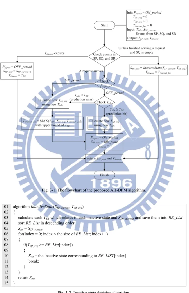
The stochastic-based algorithm proposed by Benini et al. [14] uses stochastic processes to model the behaviors of the Service Requester (SR), Service Queue (SQ), and Service Provider (SP). The overall system architecture for the DPM is shown in Fig. 2-2 [14]. The SR will send a request to the SP. When the SP is busy and if requests keep coming, incoming requests will be stored in the SQ. If the SQ is full, incoming requests will be discarded. The Power Manager (PM) observes the status of the SR, SQ, and SP, and it decides which command, such as shutdown, wakeup, or state-transition, will be sent to the SP. The probability models used to describe the behaviors of the SR, SQ, and SP are the main issue of the stochastic-based schemes. The more precise the probability models that describe the SR, SQ, and SP, the more accurate the state transition decisions made by the PM, thus saving more energy of the system.

The following are representative stochastic-based algorithms. In [14], it models request arrival and state transition as stationary discrete-time Markov processes. The assumptions of this approach are as follows [14]:

1. The arrival of service requests can be modeled by an m-memory Markov chain. The

m-memory Markov model has 2m _{states, one for each possible sequence of consecutive}

bits.

2. The state transition delays in the SP can be modeled as random variables with a geometric distribution.

3. Model parameters and cost functions are available and accurately measured before

However, the above constraints are not likely to occur in real life. First, in most cases, the arrivals of user requests, the state transition delays, and even the service time, are non-stationary [15]. Second, the characteristic of discrete time causes additional cost for the PM because the PM must periodically wakeup to do computation. The first drawback can be dealt with using a non-stationary stochastic process, and the second drawback can be handled by changing the time from discrete to continuous [16][18].

For the first drawback, Chung et al. [16] proposed an approach using a non-stationary stochastic process to model the arrival distribution of user requests. They proposed a mechanism called sliding window to keep historical data. The sliding window is limited in length and hence recent historical data are kept in order to reflect recent user request behavior. Because the distribution of user requests is non-stationary, the decision table of the SP must be recalculated in every period. To overcome this drawback, the authors used table lookup and interpolation to calculate the decision table to avoid the recalculation. Ren et al. [17] modified the approach in [16] and introduced a multi-mode model using a Markov-modulated stochastic process to model the non-stationary arrival process of service requests [17]. The advantage of these two approaches is that the request arrival distribution of the SR can be adapted to any distribution. But the disadvantages are an enormous amount of memory usage and computation power required. If we apply these two approaches to several components in a mobile device, we have to derive a request arrival distribution for each component in advance and it will be time consuming and inconvenient.

As to the second drawback, Qiu et al. [18] proposed a continuous-time Markov decision process to decrease the computation of the PM. In this approach, the decision is made on an event arrival, such as a user request arrival, the SP starting to serve a user request, and the SP finishing a user request. Rong et al. [19] extended the work in [18] to model a battery-powered portable system by introducing and incorporating a new continuous-time Markovian decision process model of the battery source [19]. There are some disadvantages in this approach. First, the computation complexity both in time and space are high because of the characteristic of continuous-time based policy optimization. Second, the experiment was based on a continuous-time Markov process, that means that the inter-arrival time of user requests, the switching time of the SP, and the state transition of the SQ are exponential distributed, which are not quite realistic in the real world. In [20], the authors proposed a Variation Aware DPM, which is based on the Partially Observable Markov Decision Process, to solve the power management problem on chip multiprocessor (CMP) architectures. The algorithm has a belief state estimator, which estimates the next state of the system, and a

policy maker, which assigns optimal actions to the CMP [20]. The time complexity of the

algorithm is O(nm), where n is the number of states and m is the number of actions [20]. The time complexity is high compared with timeout-based and predictive-based algorithms.

2.4 Machine learning algorithms

Several researchers applied machine learning to learn the request arrival patterns of the SR. Dhiman et al. [21] and Prabha et al. [22] proposed expert based machine learning

algorithms. An expert based machine learning algorithm selects the best DPM policy from a set of DPM policies. These policies are called experts. Each expert has a weight value which indicates the expert's priority and is adjustable by the machine learning algorithm. The weight value will be adjusted in every idle period and the expert with the highest weight value in the current idle period will be used to control an embedded system during the next idle period. However, the performance of an expert based machine learning algorithm is highly dependent on chosen experts. In [23], the authors proposed a reinforcement learning based algorithm. The algorithm is based on the Q-learning algorithm, which was originally designed to find a policy for a Markov Decision Process, to learn the arrival request patterns of the SP [23]. The authors modified the Q-learning algorithm to solve the DPM problem and speed up the algorithm's convergence time by updating more than one Q values simultaneously. The time complexity of the modified Q-learning algorithm is O(|SP| × |A|), and the space complexity is

O(|SP| × |SQ| × |SR| × |A|), where |SP|, |SQ|, and |SR| are the number of states of the SP, SQ,

and SR, respectively, and |A| is the number of commands. In [24], the authors combine fuzzy decision processes and reinforcement learning. The authors use the fuzzy decision processes to model the behavior of the wireless sensor nodes, and adapt the modified Q-learning algorithm to decide a sequence of duty cycles in order to improve energy efficiency. Note that the time and space complexities of the modified Q-learning algorithm are higher than those of the proposed AH-DPM algorithm, which are constant in both time and space complexity, which will be explained later.

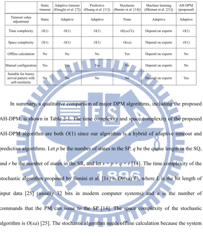
In summary, a qualitative comparison of major DPM algorithms, including the proposed AH-DPM, is shown in Table 2-1. The time complexity and space complexity of the proposed AH-DPM algorithm are both O(1) since our algorithm is a hybrid of adaptive timeout and predictive algorithms. Let p be the number of states in the SP, q be the queue length in the SQ, and r be the number of states in the SR, and let x = p × q × r [14]. The time complexity of the stochastic algorithm proposed by Benini et al. [14] is O((xa)3_{L), where L is the bit length of}

input data [25] (usually 32 bits in modern computer systems) and a is the number of commands that the PM can issue to the SP [14]. The space complexity of the stochastic algorithm is O(xa) [25]. The stochastic algorithm needs offline calculation because the system state transition matrix must be calculated in advance. Because the machine learning algorithm uses experts, which are a set of DPM algorithms, the time and space complexities, offline calculation, and manual configuration are dependent on the selected DPM algorithms. In addition, STO, ATO, and predictive algorithms need to configure some initial values manually.

Table 2-1. A qualitative comparison of representative DPM algorithms.

Static

timeout (Douglis et al. [7]) Adaptive timeout (Huang et al. [11]) Predictive (Benini et al. [14]) Stochastic (Dhiman et al. [21]) Machine learning (proposed) AH-DPM Timeout value

adjustment Static Adaptive Adaptive None Adaptive Adaptive Time complexity O(1) O(1) O(1) O((xa)3_{L) Depend on experts O(1)}

Space complexity O(1) O(1) O(1) O(xa) Depend on experts O(1)

Offline calculation No No No Yes Depend on experts No Manual configuration Yes Yes Yes No Depend on experts No

Suitable for bursty arrival pattern with

arrival patterns with self-similarity. They are more suitable for stationary request arrival patterns.

Chapter 3

Proposed AH-DPM Algorithm

3.1 The design of the proposed algorithm

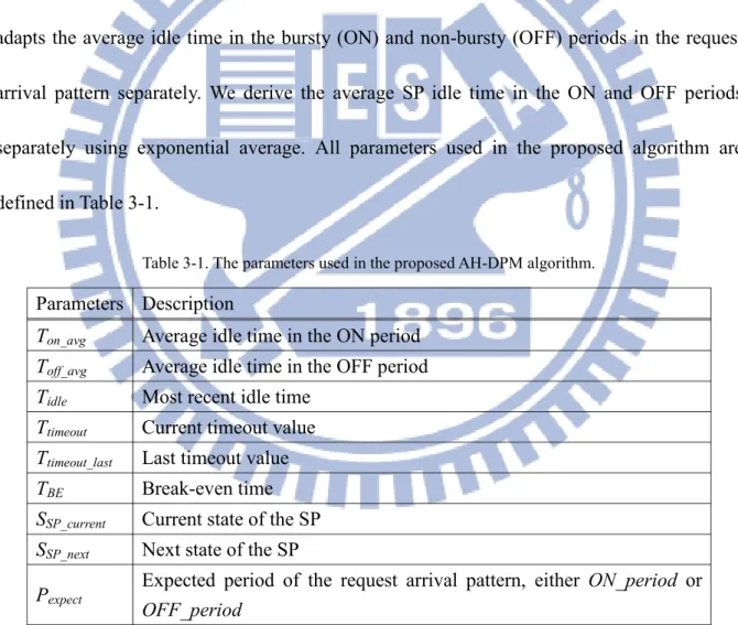
To obtain better power saving of the SP, the proposed AH-DPM algorithm handles and adapts the average idle time in the bursty (ON) and non-bursty (OFF) periods in the request arrival pattern separately. We derive the average SP idle time in the ON and OFF periods separately using exponential average. All parameters used in the proposed algorithm are defined in Table 3-1.

The proposed AH-DPM algorithm returns two values: the next state, SSP_next, that the SP

Table 3-1. The parameters used in the proposed AH-DPM algorithm.

Parameters Description

Ton_avg Average idle time in the ON period

Toff_avg Average idle time in the OFF period

Tidle Most recent idle time

Ttimeout Current timeout value

Ttimeout_last Last timeout value

TBE Break-even time

SSP_current Current state of the SP

SSP_next Next state of the SP

Pexpect Expected period of the request arrival pattern, either ON_period or

the next state. There are three main ideas in the proposed AH-DPM algorithm: (1) keeping track of the average idle time in the ON period, Ton_avg, and in the OFF period, Toff_avg,

separately, (2) using the average idle time in the ON period to adjust the timeout value more precisely and using the average idle time in the OFF period to decide which inactive state the SP should be switched to, and (3) comparing the most recent idle time, Tidle, with the

break-even time, TBE, to determine whether the expected period of the request arrival pattern,

Pexpect, is ON_period or OFF_period. Three cases will be monitored by the proposed

AH-DPM algorithm:

1. When a request arrives, based on Pexpect and the comparison between Tidle and TBE, there

are three situations required to be taken care of:

a. If Pexpect equals to ON_period, calculate new Ton_avg using new Tidle. Then, Ttimeout_last is

updated to the maximum value among Ttimeout_last, Tidle, and Ton_avg, with upper bound

of TBE.

b. If Pexpect equals to OFF_period, and Tidle is smaller than TBE, this situation is called

prediction miss because in the OFF period, Tidle should be larger than TBE. In this case,

the calculations described in situation 1a will be performed since Pexpect should be in

the ON period.

c. If Pexpect equals to OFF_period, and Tidle is larger than or equal to TBE, this situation is

called prediction hit. Toff_avg will be calculated using new Tidle.

will be set to idle state, and SSP_next along with timeout value of zero will be returned. The

reason for returning zero as the timeout value is to wake up the SP immediately whenever there is a request arrived and the SP is in an inactive state.

2. When the SP has finished serving a request and the SQ is empty, the SP may be inactivated since there is no request to be served. The next state of the SP, SSP_next, will be

chosen by the algorithm InactiveState. Then, SSP_next and Ttimeout will be returned.

3. When Ttimeout expires, the SP will be switched to the state indicated by SSP_next, and Pexpect

will be set to OFF_period to indicate that the request arrival pattern is now in the OFF period. In the meantime, if the SP has deeper inactive states, which implies lower power consumption and higher state transition overhead, the next deeper inactive state, relative to the current inactive state, of the SP will be assigned to SSP_next, and Ttimeout will be set to

TBE. The SP will be switched to a deeper inactive state specified in SSP_next when Ttimeout

expires. This timeout iteration mechanism repeats until the SP is switched to the deepest inactive state if there is no incoming request arrival for a long time.

In summary, the benefits of the proposed AH-DPM algorithm are that our algorithm adapts to bursty request arrival patterns with self-similarity and a service provider (SP, i.e., hard disk or WLAN NIC, in this dissertation) with multiple inactive states by the following two steps to achieve better power saving. First, it derives the average idle time of the SP in the bursty (ON) period and non-bursty (OFF) period separately. Second, it uses the average idle time in the ON period to adjust the timeout value more precisely and uses the average idle

time in the OFF period to decide which inactive state the SP should be switched to. In other words, the calculation of the timeout value described in situation 1a above is to set the timeout value long enough to prevent an unexpected SP state transition to an inactive state and to keep the timeout value short enough to decrease the length of the busy wait period during the ON period.

3.2 The flowchart and pseudo codes of the proposed

algorithm

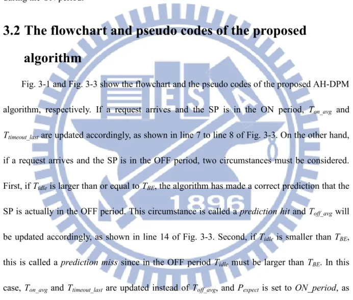
Fig. 3-1 and Fig. 3-3 show the flowchart and the pseudo codes of the proposed AH-DPM algorithm, respectively. If a request arrives and the SP is in the ON period, Ton_avg and

Ttimeout_last are updated accordingly, as shown in line 7 to line 8 of Fig. 3-3. On the other hand,

if a request arrives and the SP is in the OFF period, two circumstances must be considered. First, if Tidle is larger than or equal to TBE, the algorithm has made a correct prediction that the

SP is actually in the OFF period. This circumstance is called a prediction hit and Toff_avg will

be updated accordingly, as shown in line 14 of Fig. 3-3. Second, if Tidle is smaller than TBE,

this is called a prediction miss since in the OFF period Tidle must be larger than TBE. In this

case, Ton_avg and Ttimeout_last are updated instead of Toff_avg, and Pexpect is set to ON_period, as

shown in line 18 to line 19 of Fig. 3-3. Once a request is served and the SQ is empty, the SP becomes idle. Then, the SP will be switched to an inactive state SSP_next with timeout value

Ttimeout. SSP_next will be assigned using algorithm InactiveState, as shown in Fig. 3-2. Algorithm

each inactive state, and save it into BE_List. BE_List is an array that stores TBE of each

inactive state. BE_List is then sorted in the descending order. Toff_avg will be compared with

each TBE. If Toff_avg is greater than or equal to a certain TBE, the inactive state corresponding to

the previous TBE in BE_List will be returned to algorithm AH-DPM, as shown from line 6 to

line 14 in Fig. 3-2. If Ttimeout expires, the SP will be switched to state SSP_next and Pexpect will be

set to OFF_period. In the meantime, the timeout iteration mechanism mentioned in section 3.1 starts. A new inactive state and TBE will be set to SSP_next and Ttimeout accordingly, as shown

Fig. 3-1. The flowchart of the proposed AH-DPM algorithm.

01 algorithm InactiveState(SSP_current, Toff_avg)

02 {

03 calculate each TBE which relates to each inactive state and SSP_current, and save them into BE_List

04 sort BE_List in descending order 05 Sret = SSP_current

06 for(index = 0; index < the size of BE_List; index++) 07 {

08 if(Toff_avg >= BE_List[index])

09 {

10 Sret = the inactive state corresponding to BE_LIST[index]

11 break;

12 }

13 } 14 return Sret

15 }

01 algorithm AH-DPM(SSP_current, Tidle)

02 {

03 if(a request arrives) 04 {

05 if(Pexpect == ON_period)

06 {

07 Ton_avg = α × Tidle + (1 - α) × Ton_avg

08 Ttimeout_last = MAX(Tidle, Ton_avg, Ttimeout_last), with upper bound of TBE

09 }

10 else if(Pexpect == OFF_period)

11 {

12 if(Tidle ≥ TBE) /* prediction hit */

13 {

14 Toff_avg = α × Tidle + (1 - α) × Toff_avg

15 }

16 else /* prediction miss */

17 {

18 Ton_avg = α × Tidle + (1 - α) × Ton_avg

19 Ttimeout_last = MAX(Tidle, Ton_avg, Ttimeout_last), with upper bound of TBE

20 } 21 } 22 Pexpect = ON_period 23 SSP_next = Idle_state 24 Ttimeout = 0 25 }

26 else if(SP has finished serving a request and SQ is empty) 27 {

28 SSP_next = InactiveState(SSP_current, Toff_avg)

29 Ttimeout = Ttimeout_last

30 }

31 else if(Ttimeout is expired)

32 {

33 Pexpect = OFF_period

34 SSP_next = SSP_current+1

35 Ttimeout = TBE

36 }

37 Return SSP_next and Ttimeout

38 }

Chapter 4

Experimental Results and Discussion

4.1 Experimental setup

We compare our algorithm (AH-DPM) with the oracle algorithm (Oracle), the static timeout algorithm (STO) with timeout value of 30 seconds [2], the adaptive timeout algorithm (ATO) of Douglis et al. [7] with parameters (αm, βm, ρ) = (0.5, 1.5, 0.1) [2] and initial timeout

value of 30 seconds [2], the predictive algorithm (Predictive) of Huang et al. [11] with parameters α = 0.3 and c = 2 [2], the stochastic (Stochastic) algorithm of Benini et al [14], and the machine learning (ML) algorithm of Dhiman et al [21]. Remind that the oracle algorithm is a theoretically optimal algorithm because it knows the arrival time of all requests; therefore, the algorithm can determine exactly when and to which state the SP should be switched for power saving. The Stochastic algorithm does not need to set any initial value, but the optimal decision policies must be calculated in advance. The ML algorithm uses STO, ATO, Predictive, and Stochastic algorithms as its experts. The parameters of each expert used in the ML algorithm are same as those listed above. Since the oracle algorithm is aware of all the requests issued from the beginning to the end, it can come out with the most power efficient results. The AlwaysOn algorithm is defined as “always keeping the SP in the active state,” and represents the worst case of average power consumption and the best case of average response

time (average packet transmission delay) in hard disk (WLAN NIC) experiments.

In the hard disk experiments, we used a typical hard disk specification of Hitachi Travelstar 5K100 as an example SP specification, as shown in Table 4-1 and Table 4-2 [26]. The state transition diagram of Hitachi Travelstar 5K100 is shown in Fig. 4-1. Note that state transitions between Performance Idle, Active Idle, and Low Power Idle are hardware controlled; thus cannot be controlled by the user or operating system. We use dotted lines to represent the hardware-controlled state transitions. The hard disk request traces were collected for a week by monitoring the ATA commands sent and received by libATA drivers under Fedora 12 [27], kernel version 2.6.32.11 [28]. The trace characteristics of hard disk requests for each day of the week are listed in Table 4-3. We compare the average power consumption and average response time for the hard disk among these DPM algorithms. The average power consumption is measured in Watt, and it is defined as total energy consumed divided by total elapsed time. The average response time is measured in millisecond and it is defined as the average elapsed time between a request arrived and the request having been served, which includes the queuing delay and service time of a request.

As to the WLAN NIC experiments, we used the specification of the Intel PRO/Wireless 3945ABG (802.11g) card, which is shown in Table 4-4 [29]. However, the state transition time and state transition power of the Intel PRO/Wireless 3945ABG card are not available. We used the state transition time listed in [30]. The state transition power from sleep to idle is set to twice of the power consumption in idle state, and the state transition power from idle to

sleep is set to the power consumption in sleep state [31]. The state transition characteristics of the WLAN NIC are listed in Table 4-5, and the associated state transition diagram is illustrated in Fig. 4-2. In addition, the real traces of the WLAN NIC were captured using Wireshark [32], version 1.2.6, under Fedora 12 [27]. The trace characteristics of WLAN NIC packets for each day of the week are listed in Table 4-6. The average power consumption and

average packet transmission delay are metrics of the WLAN NIC for performance evaluation

among these DPM algorithms. The definition of the average power consumption is identical to that for the hard disk and the average packet transmission delay is measured in millisecond, and it is defined as the queuing delay plus the packet transmission time.

Finally, we also evaluate the prediction miss rate and the inactivation ratio, which will be defined later. The prediction miss rate can reflect the average power consumption and the inactivation ratio can reflect the average response time in the hard disk and the average transmission delay in the WLAN NIC. There are two cases of prediction miss: false positive

prediction and false negative prediction. A positive prediction is that the PM decides to

inactivate the SP, and a negative prediction is that the PM decides NOT to inactivate the SP. Therefore, the false positive prediction occurs in a situation that the PM inactivates the SP (i.e., switching the SP to a lower power consumption state), but the length of the inactive period is shorter than the break-even time. That is, the SP should not be inactivated, but it is inactivated. The false negative prediction occurs in a situation that the PM keeps the SP in active state, but the length of the idle period is longer than the break-even time. That is, the SP should be inactivated, but it is not inactivated. Both cases will result in extra power

consumption penalty. According to the definitions of false positive prediction and false negative prediction, the definition of the prediction miss rate Rprediction_miss is as follows:

𝑅

𝑝𝑝𝑝𝑝𝑝𝑝𝑝𝑝𝑝𝑛_𝑚𝑝𝑚𝑚

=

𝑁𝑓𝑓_𝑚𝑚𝑚𝑚_{𝑁𝑓𝑝𝑝𝑝𝑚𝑝𝑝𝑚𝑝𝑓}+𝑁𝑓𝑓_𝑚𝑚𝑚𝑚 (2)

where Nfp_miss is the number of false positive prediction, Nfn_miss is the number of false negative

prediction, and Nprediction is the total number of predictions made by the PM. The definition of

the inactivation ratio Rinactivate is defined as follows:

𝑅

𝑝𝑛𝑖𝑝𝑝𝑝𝑖𝑖𝑝𝑝

=

_𝑁𝑁_{𝑓𝑝𝑝𝑝𝑚𝑝𝑝𝑚𝑝𝑓}𝑚𝑓𝑖𝑝𝑝𝑚𝑖𝑖𝑝𝑝 (3)

where Ninactivate is the number of switching the SP from the active state to an inactive state (a

lower power consumption state). When the SP is in an inactive state and a request arrives, the SP must switch to the active state in order to serve the request. Since existing DPM algorithms, except the oracle algorithm, did not actually implement the pre-wakeup mechanism, an incoming request will be queued in the SQ waiting for the SP to be switched from an inactive state to the active state. Therefore, it results in queuing delay. Since each SP’s inactivation will lengthen the queuing delay of the next incoming request, the higher the inactivation ratio is, the longer the average response time of the hard disk and the average packet transmission delay of the WLAN NIC are.

Table 4-1. State transition time and power consumption specifications of Hitachi Travelstar 5K100 hard disk [26].

From To Time _(sec) Power consumption _(Watt)

Sleep Performance Idle 3.5 3.8

Standby Performance Idle 2.5 3.8

Low Power Idle Performance Idle 0.3 2.0 Active Idle Performance Idle 0.02 2.0

Performance Idle Standby 0.35 2.0

Performance Idle Sleep 0.35 2.0

Table 4-2. Power consumption specification of Hitachi Travelstar 5K100 hard disk [26].

State Power consumption _(Watt) Performance Idle 2.0

Active Idle 1.1

Low Power Idle 0.65

Read 2.0

Write 2.0

Seek 2.5

Standby 0.2

Sleep 0.1

Table 4-3. Trace characteristics of hard disk requests.

Day of Week Number of

Requests

𝑇

𝑅𝑅

𝜎

𝑇𝑅𝑅 Sunday 148175 0.5826582132 28.066745610 Monday 273503 0.3158121481 7.576979263 Tuesday 90081 0.9588597164 13.238787090 Wednesday 190393 0.4537697663 7.577420349 Thursday 532259 0.1623176762 3.813604001 Friday 128420 0.6725806881 10.876428390 Saturday 46820 1.8449750100 18.263384880 A week 1409651 0.4289868597 11.847667333

𝑇𝑅𝑅: Average request inter-arrival time (sec)

𝜎𝑇𝑅𝑅: Standard deviation of the request inter-arrival time

Table 4-4. Power consumption specification of Intel PRO/Wireless 3945ABG WLAN NIC [29].

State Power consumption _(Watt)

Transmit 1.8

Receive 1.4

Idle 0.15

Sleep 0.03

Table 4-5. State transition time and power consumption of the WLAN NIC [29][30]. From To _(μsec) Time Power consumption _(Watt)

Sleep Idle 250 0.3

Idle Sleep 80 0.03

4.2 Experimental results

Fig. 4-3 shows the experimental results of the average power consumption of the hard disk for each DPM algorithm on each day of a week. In Fig. 4-3, we found that the proposed AH-DPM algorithm is always better than the other algorithms except the oracle algorithm under the request trace of each day in a week. By observing Table 4-3 and Fig. 4-3, we found that average power consumption is proportional to number of requests, except the case on Tuesday. The average power consumption on Tuesday is still higher in spite of a lower number of requests. This is because of a higher inactivation ratio on Tuesday, as shown in Fig. 4-5. Since a higher inactivation ratio implies a higher number of state transitions, the power consumption increases due to frequent state transitions. As to the average response time, Fig. 4-4 shows that the proposed AH-DPM algorithm is larger than the ATO, AlwaysOn, ML, Oracle, and STO algorithms, and is shorter than the Predictive algorithm. By observing Fig. 4-4 and Fig. 4-5, we found that average response time is proportional to inactivation ratio. This is because that if the SP is in an inactivated state and there is an incoming request, the SP

Table 4-6. Trace characteristics of WLAN NIC traffic.

Day of Week Number of

Requests

𝑇

𝑃𝑅

𝜎

𝑇𝑃𝑅 Sunday 68812 1.2524797900 13.271983260 Monday 24697 3.0321168550 43.423190660 Tuesday 48308 1.6348761390 218.246429500 Wednesday 115253 0.7495722815 10.870117770 Thursday 183500 0.4701362994 8.127996827 Friday 13013 6.5880108190 73.593723700 Saturday 8164 10.4842361800 93.448664130 A week 461747 1.2648289645 73.980365017

𝑇𝑃𝑅: Average packet inter-arrival time (sec)

must be switched to the active state to serve the request. Since no existing DPM algorithms have the ability to switch the SP to the active state in advance, the request must be queued in the SQ to wait for the SP to switch from an inactive state to the active state. Therefore, a larger inactivation ratio will result in longer response time.

Fig. 4-4. Comparisons of the average response time of the hard disk.

Fig. 4-6 and Fig. 4-7 are the comparison of average power consumption and average response time in a week for the hard disk, respectively. In Fig. 4-6, we observed that the average power consumption of the proposed AH-DPM is 30.41% worse than that of the oracle algorithm, and is better than that of the ATO, ML, Predictive, STO, and Stochastic algorithms by 78.34%, 99.28%, 124.97%, 93.45%, and 294.63%, respectively. That is, the proposed AH-DPM algorithm performed the best except the oracle algorithm in terms of average power consumption. Remind that the oracle algorithm is theoretically optimal. Since the prediction miss will cause extra power consumption, we derive the prediction miss rate of each algorithm. In Fig. 4-8, we found that the prediction miss rate of the proposed AH-DPM algorithm is the lowest compared to that of the other DPM algorithms except the oracle algorithm. The results are in accordance with those illustrated in Fig. 4-6. Although the average response time of the proposed AH-DPM algorithm in Fig. 4-7 is not the best, it is still lower than that of the Predictive algorithm by 33.04% and it is also lower than the average disk access time specified in a hard disk specification [26]. According to this specification [26], the average response time for read/write one byte from/to the hard disk is about 20.5 ms (command overhead + average seek time + average latency + average disk-buffer data transfer rate). Therefore, the average response time of the proposed AH-DPM algorithm, which is 19.375 ms as shown in Fig. 4-7, is lower than 20.5 ms, and it meets the hard disk specification.

Fig. 4-6. Comparison of the average power consumption of the hard disk in a week.

We also evaluate the average power consumption and average packet transmission delay on each day of a week for each DPM algorithm. In Fig. 4-9, we found that the average power consumption of the proposed AH-DPM is comparable to that of the ATO, Oracle, and Predictive algorithms, and is better than that of the ML, STO, and Stochastic algorithms. However, in terms of average packet transmission delay, the proposed AH-DPM algorithm is better than the ATO and Predictive algorithms, as shown in Fig. 4-10. Fig. 4-11 illustrates the inactivation ratio of the WLAN NIC. Through Fig. 4-10 and Fig. 4-11, we can confirm that the average transmission delay is also proportional to the inactivation ratio except the Saturday case. This is because the average packet arrival rate is low on that Saturday, which can be observed from Table 4-6. Lower average packet arrival rate implies less bursty of the packet arrival pattern, which leads to the decrease of the queuing delay caused by bursty

Fig. 4-9. Comparisons of average power consumption of the WLAN NIC.

Fig. 4-12 and Fig. 4-13 illustrate the average power consumption and average packet transmission delay of the WLAN NIC in a week for different DPM algorithms, respectively. In Fig. 4-12, we observed that the average power consumption of the AH-DPM algorithm is comparable to (0.7% more than) that of the ATO, Oracle, and Predictive algorithms, and is better than that of the ML, STO, and Stochastic algorithms by 169.99%, 89.14%, and 369.01%, respectively. Note that although the prediction miss rate of the proposed AH-DPM algorithm is the best, as shown in Fig. 4-14, compared with the other algorithms except the oracle algorithm, the average power consumption of the AH-DPM algorithm is still slightly larger than that of the ATO and Predictive algorithm. This is because that the average timeout value of the AH-DPM algorithm is larger than that of the ATO and Predictive algorithms, as

illustrated in Fig. 4-15. That is, the proposed AH-DPM has a higher prediction hit rate that can reduce more power consumption (see Fig. 4-12) and decrease more packet transmission delay (see Fig. 4-13); however, the minor penalty is a longer timeout value that causes slightly larger power consumption.

As to the average packet transmission delay, Fig. 4-13 shows that the proposed AH-DPM algorithm is better than the ATO and Predictive algorithms by 23.22% and 25.18%, and is worse than the ML, STO, and Stochastic algorithms by 41.36%, 41.05%, and 38.22%, respectively.

Fig. 4-13. Average packet transmission delay of the WLAN NIC in a week.

In summary, considering the tradeoff between average power consumption and average response time (average packet transmission delay), the proposed AH-DPM algorithm performs the best among the DPM algorithms, except the oracle algorithm, for the hard disk and the WLAN NIC. Since our work derives the average idle time in the ON period and OFF period separately and uses the average idle time in the ON period to determine the timeout value, we can set the timeout value long enough to decrease the false positive prediction miss rate and keep the timeout value short enough to decrease the false negative prediction miss rate. By decreasing these two types of prediction miss rates, the proposed algorithm can reduce unnecessary power consumption of the SP. In addition, the proposed algorithm also adapts to the SP that has multiple inactive states by using the average idle time in the OFF period to decide which inactive state the SP should be switched to. Such adaptation can

further decrease the power consumption of the SP because we can choose a better inactive state according to the average idle time in the OFF period. The longer idle time of the SP in the OFF period, the deeper inactive state the SP can be switched to.

4.3 Discussion

In Fig. 4-4, we observed that the average response time on Tuesday and Saturday are higher than that in the other days. This is because that the average request inter-arrival time on Tuesday and Saturday are longer than those on the other days, as shown in Table 4-3. A longer average request inter-arrival time implies a higher probability to inactivate a component. Because of lacking the pre-wakeup mechanism for each DPM algorithm, except the Oracle algorithm, the SP will only be waked up when a request arrived. Therefore, the average response time will increase due to the state transition time penalty while waking up the SP.

The performance of the ATO algorithm [7] is highly correlated with the SP’s state transition time from an inactive state to the active state, called wakeup state transition time, and the request arrival pattern. The ATO algorithm will increase the timeout value if the wakeup state transition time of the SP is larger than the latest idle time of the SP, and will decrease the timeout value otherwise. If the wakeup state transition time is smaller (larger) than the idle time in a period with bursty request arrivals, the ATO algorithm will decrease (increase) the timeout value rapidly. For the hard disk, since the wakeup state transition time, which are 3.5 seconds from Sleep to Performance Idle and 2.5 seconds from Standby to Performance Idle (see Table 4-1), is larger than the idle time of the SP during a bursty request

arrivals period, it will cause the timeout value to be increased rapidly. A larger timeout value means a lower probability to inactivate the SP, which results in higher power consumption of the ATO algorithm. As to the WLAN NIC, the wakeup state transition time of the ATO algorithm, which is 80 μs (see Table 4-5), is smaller than the idle time of the SP during a bursty request arrivals period, and it causes the timeout value to be decreased rapidly. A smaller timeout value causes a larger inactivation ratio as well as a larger false positive prediction miss rate, which result in longer packet transmission delay.

The Predictive algorithm [11] also suffers from the bursty request arrivals pattern. This is because that the Predictive algorithm uses equation (1) (refer to Chapter 2) to predict the idle time. If the predicted idle time is longer than the break-even time, the SP will be inactivated. Otherwise, the SP will remain in the active state. When a request arrives, the PM will recalculate and update the predicted idle time. If the request arrival pattern is bursty and the idle time of the SP in the bursty period is shorter than the break-even time, the average idle time will be shortened rapidly and will be smaller than the break-even time. When the average idle time is shorter than the break-even time, the SP will remain in the active state until the average idle time becomes larger than the break-even time, even if the next idle time is longer than the break-even time. This situation of the SP remaining in the active state while the actual idle time is longer than the break-even time will cause extra power consumption. Although the Predictive algorithm uses a watchdog mechanism to compensate the prediction inaccuracy caused by the bursty request arrivals pattern, the busy wait period caused by the watchdog mechanism will also result in extra power consumption.

The ML algorithm [21] has a drawback that is caused by the calculation of a weight factor for each expert. The weight of each expert is calculated as follows:

𝑤

_𝑝𝑝+1

= 𝑤

_𝑝𝑝

𝛽

𝑙_𝑚𝑝

₍₄₎

where 𝑤𝑝𝑝 is the weight factor of expert i, β is a chosen value between 0 and 1, which was

assigned to 0.75 in the experiments [21] , and 𝑙𝑝𝑝 is the joint loss factor, which is given by:

𝑙

_𝑝𝑝

_{= 𝛼 × 𝑙}

𝑝𝑝𝑝

+ (1 − 𝛼) × 𝑙

𝑝𝑝𝑝

(5)

where 𝑙_𝑝𝑝𝑝 _{and 𝑙} 𝑝𝑝

𝑝 _{are the loss factors corresponding to energy savings and performance}

delay for an expert i [21]. Because β is between 0 and 1 and lit is always positive, the weight will approach to zero after a series of calculation, which will cause the underflow problem. If this problem happens, the weight of each expert will be the same and the result of selecting an operational expert will be the same.

Finally, the performance of the Stochastic algorithm is not good because the request arrival pattern of the SR is bursty. With the bursty request arrival patterns of the hard disk and WLAN NIC, the state transition policies calculated by the Stochastic algorithm will tend to keep the SP in the active state and it will result in high average power consumption.

Chapter 5

Conclusions and Future Work

5.1 Concluding remarks

In this dissertation, we have presented a power efficient adaptive hybrid dynamic power management (AH-DPM) algorithm that adapts to the self-similar workloads with bursty nature of the SPs (hard disk and WLAN NIC) in mobile devices to lengthen their battery lifetime. To adapt to bursty request arrival patterns with self-similarity of hard disks or WLAN NICs, the proposed AH-DPM first derives the average idle time of the SP in the bursty (ON) period and non-bursty (OFF) period separately. Then, to achieve better power saving, we use the average idle time in the ON period to adjust the timeout value more precisely and use the average idle time in the OFF period to decide which inactive state the SP should be switched to. Experimental results based on real traces of a hard disk have shown that the average power consumption of the proposed AH-DPM is better than that of the ATO, ML, Predictive, STO, and Stochastic algorithms by 78.34%, 99.28%, 124.97%, 93.45%, and 294.63%, respectively. Nevertheless, the proposed AH-DPM algorithm did not sacrifice the average response time of the hard disk too much, which is still lower than the average disk access time specified in a hard disk specification. In addition, experimental results based on real traces of a WLAN NIC have also shown that the average power consumption of the

proposed AH-DPM is comparable to that of the ATO, Oracle, and Predictive algorithms, and is better than that of the ML, STO, and Stochastic algorithms by 169.99%, 89.14%, and 369.01%, respectively. As to the average packet transmission delay, the proposed AH-DPM algorithm is better than that of the ATO and Predictive algorithms by 23.22% and 25.18%, and is worse than that of the ML, STO, and Stochastic algorithms by 41.36%, 41.05%, and 38.22%, respectively. In summary, the experimental results have supported that the proposed AH-DPM algorithm can provide a better tradeoff between average power consumption and average response time (average packet transmission delay) for hard disks (WLAN NICs), and thus is very feasible to ever increasing mobile devices for extending their battery lifetime.

5.2 Future work

Since large scale real traces are not easy to obtain, applying various parameter settings to an ON-OFF traffic generator to generate different request traces to thoroughly evaluate the feasibility of the proposed AH-DPM algorithm is worth to further study. Although our request traces were collected from real traces, the experiments were performed through computer simulation. Therefore, the feasibility of applying the proposed AH-DPM algorithm to mobile devices equipped with hard disks and WLAN NICs through a testbed also deserves to further research. Since the solid-state drive (SSD) has some good characteristics, such as low energy consumption, noiseless, and low temperature, compared with the tradition hard drive, the possibility of applying the proposed AH-DPM algorithm to mobile devices equipped with the SSD is worth to further investigate. In addition, applying the proposed AH-DPM algorithm to

Bibliography

[1] Y. H. Lu and G. De Micheli, “Comparing system level power management policies,”

IEEE Des. Test. Comput., vol. 18, pp. 10-19, March-April 2001.

[2] Y. H. Lu, E. Y. Chung, T. Simunic, T. Benini, and G. De Micheli, “Quantitative comparison of power management algorithms,” in Proc. IEEE DATE, 2000, pp. 20-26. [3] K. Zhang, X. Ge, C. Liu, and L. Xiang, “Analysis of frame traffic characteristics in

IEEE 802.11 networks,” in Proc. IEEE ChinaCOM, Aug. 2009, pp. 1-5.

[4] L. Xiang, X. Ge, K. Zhang, and C. Liu, "A self-similarity frame traffic model based on the frame components in 802.11 networks," in Proc. IEEE CSE, 2009, vol. 2, pp. 955-960.

[5] M. E. Gomez and V. Santonja, "Self-similarity in I/O workload: analysis and modeling," in Proc. IEEE WWC, 1998, pp. 97-104.

[6] M. E. Gomez and V. Santonja, "Analysis of self-similarity in I/O workload using structural modeling," in Proc. IEEE MASCOT, 1999, pp. 234-242.

[7] F. Douglis, P. Krishnan, and B. Bershad, “Adaptive disk spin-down policies for mobile computers,” in Proc. 2nd USENIX Symp. On Mobile and Location-independent

Computing, 1995, vol. 8, pp. 381-413.

[8] C. M. Olsen and C. Narayanaswarni “PowerNap: an efficient power management scheme for mobile devices,” IEEE Trans. Mobile Comput., vol. 5, no. 7, pp. 816-828, July 2006.

[9] L. Benini, A. Bogliolo, and G. De Micheli, “A survey of design techniques for system-level dynamic power management,” IEEE Trans. VLSI Syst., vol. 8, pp. 299-316, June 2000.

[10] M. B. Srivastava, A. P. Chandrakasan, and R. W. Brodersen, “Predictive system shutdown and other architectural techniques for energy efficient programmable computation,” IEEE Trans. VLSI Syst., vol. 4, pp. 42-55, March 1996.

[11] C. H. Hwang and A. C. H. Wu, “A predictive system shutdown method for energy saving of event-driven computation,” ACM TODAES, vol. 5, pp. 226-241, April 2000. [12] E. Y. Chung, L. Benini, and G. De Micheli, “Dynamic power management using

adaptive learning tree,” in Proc. IEEE/ACM ICCAD, 1999, Digest of Technical Papers, pp. 274-279.

[13] D. Ramanathan, S. Irani, and R.K. Gupta, “An analysis of system level power management algorithms and their effects on latency,” IEEE Trans. Computer-Aided

Design, vol. 21, pp. 291-305, March 2002.

[14] L. Benini, A. Bogliolo, G. A. Paleologo, G. De Micheli, “Policy optimization for dynamic power management,” IEEE Trans. Computer-Aided Design Integr. Circuits

Syst., vol. 18, pp. 813-833, June 1999.

[15] S. Irani, S. Shukla, and R. Gupta, “Online strategies for dynamic power management in systems with multiple power-saving states,” ACM TECS., vol. 3, no. 2, pp. 325-346, Aug. 2003.

[16] E. Y. Chung, L. Benini, A. Bogliolo, Y. H. Lu, and G. De Micheli, “Dynamic power management for nonstationary service requests,” IEEE Trans. Comput., vol. 51, pp. 1345-1361, Nov. 2002.

[17] Z. Ren, B. H. Krogh, and R. Marchlescu, “Hierarchical adaptive dynamic power management,” IEEE Trans. Comput., vol. 54, pp. 409-420, April 2005.

[18] Q. Qiu, Q. Wu, and M. Pedram, “Stochastic modeling of a power-managed system-construction and optimization,” IEEE Trans. Computer-Aided Design Integr.

Circuits Syst., vol. 20, no. 10, pp. 1200-1217, Oct. 2001.

[19] P. Rong and M. Pedram, “Battery-aware power management based on Markovian decision processes,” IEEE Trans. Computer-Aided Design Integr. Circuits Syst., vol. 25, pp. 1337-1349, July 2006.

[20] M. Ghasemazar and M. Pedram, “Variation aware dynamic power management for chip multiprocessor architectures,” in Proc. IEEE DATE, Mar. 2011, pp. 1-6.

[21] G. Dhiman, and T. S. Rosing, “Dynamic power management using machine learning,” in Proc. IEEE/ACM ICCAD, Nov. 2006, pp. 747-754.

[22] V. L. Prabha and E. C. Monie, “Hardware architecture of reinforcement learning scheme for dynamic power management in embedded systems,” EURASIP Journal on

Embedded Systems, vol. 2007, no. 1, pp. 1-6, Jan. 2007.

[23] Y. Tan, W. Liu, and Q. Qiu, "Adaptive power management using reinforcement learning," in Proc. IEEE/ACM ICCAD, 2009, pp. 461-467.

[24] C. T. Liu and R. C. Hsu, “Dynamic power management utilizing reinforcement learning with fuzzy reward for energy harvesting wireless sensor nodes,” in Proc. IEEE IECON, Nov. 2011, pp. 2365-2369.

[25] Y. Ye, Interior point algorithms: theory and analysis. New York, NY: John Wiley & Sons, 1997, pp. 147-177.

[26] Hitachi Global Storage Technologies, “Hard Disk Drive Specification Hitachi Travelstar 5K100 2.5 inch ATA/IDE hard disk drive,” Available:

http://www.hitachigst.com/tech/techlib.nsf/techdocs/98F75D1B2B25C42F86256EBC00 65A2F9/$file/T5K100_sp.pdf.

[28] Linux Kernel Organization, Inc., “The linux kernel archives,” Available: http://www.kernel.org/.

[29] Hewlett-Packard Development Company, L.P., “The Intel PRO/Wireless 3945ABG (802.11a/b/g) Card Specification,” Available:

http://h18000.www1.hp.com/products/quickspecs/12510_div/12510_div.PDF

[30] L.Y. Zhang, Ye Ge, and J. Hou, “Energy-efficient real-time scheduling in IEEE 802.11 wireless LANs,” in Proc. IEEE ICDCS, May 2003, pp. 658-667.

[31] E. S. Jung and N. H. Vaidya, “Improving IEEE 802.11 power saving mechanism,”

Wireless Networks, vol. 14, no. 3, pp. 375-391, June 2008.