Insider Trading Performance in the Taiwan Stock Market

Insider Trading Performance in the Taiwan Stock Market

Min-Hsien Chiang*

Institute of International Business, National Cheng Kung University, Taiwan

Long-Jainn Hwang

Department of International Business Management, Wu-Feng Institute of Technology, Taiwan

Yui-Chi Wu

Institute of International Business, National Cheng Kung University, Taiwan

Abstract

This paper investigates the performance of insider trading on the Taiwan Stock Exchange. In addition to a traditional single-factor model, the conditional Jensen’s alpha approach proposed by Eckbo and Smith (1998) is employed as well. We also compare performances between mutual funds and insider portfolios. The empirical results show that insider trading does not gain any abnormal returns as found in previous studies, which is robust to weighting schemes and portfolio construction methods. Moreover, mutual funds weakly outperform insider portfolios, which leads to a conjecture that insiders may seek benefits of corporate control instead of short-term trading profits.

Key words: insider trading; generalized method of moments; Jensen’s alpha JEL classification: G14; G32

1. Introduction

Whether insider trading can obtain abnormal returns has received a lot of attention both in academics and practitioners over the past few decades. Generally, insiders who are able to get access to privileged information might benefit from trades based on unpublicized and profitable news. If insiders are assured of earning abnormal returns regularly, then the efficient market in a strong form may not exist. Accordingly, legislation often requires that insiders refrain from trading on confidential information and even return short-swing profits by insiders to the company if they are found to have gained money from trading on such information. Therefore, insiders have to release confidential information before trading on such

Received September 16, 2003, revised August 31, 2004, acceptedDecember 13, 2004.

*_{Correspondence to: Institute of International Business, National Cheng Kung University, Tainan 70101,}

information. The rationale behind this legislation is to ban any manipulative or deceptive trades and to maintain a fair capital market.

Some may argue that insider trading might have a positive effect on the allocation efficiency of the capital market. Manne (1966) states that insider trading allows information to be absorbed into share prices and aligns interests among different groups of investors. In spite of disputes on the prohibition of insider trading, the main issue in this line is to examine if insider traders actually can earn abnormally greater returns than can other investors, such as liquidity and institutional traders. This issue is crucial not only in mature capital markets but also in emerging markets. Emerging markets might experience more insider trading problems on the way to becoming mature and fair capital markets since the market structures and regulations are not complete enough to make information circulation efficient. The information asymmetry due to insider trading is much more serious, especially when an emerging market experiences economic turbulence. Insiders in those companies undergoing financial distress due to economic turbulence will sell stocks before those companies go bankrupt. This substantially increases trading losses for other investors, especially liquidity traders.

Studies regarding insider trading abound in the literature. Jaffe (1974), Finnerty (1976a, 1976b), Trivoli (1980), and Seyhun (1988) find that insider trading does show abnormal returns on the New York Stock Exchange (NYSE) and the American Stock Exchange (AMEX). Seyhun (1992) reports that corporate insiders earned an annual average return of 5.1% between 1980 and 1984. This profit for insiders increases to 7% a year after 1984. Furthermore, Givoly and Palmon (1985) investigate the association between abnormal returns to insiders and subsequent disclosure of specific information for stocks listed on the AMEX. They show that there is no clear linkage between insiders’ profits and disclosure of specific news about a company. Therefore, the abnormal returns of insider trading are related to information trades themselves.

Inspired by Finnerty (1976a), Rozeff and Zaman (1988) demonstrate that insiders can obtain abnormal returns as documented by earlier studies, but the magnitude of abnormal returns is not that big after controlling for size and price/earning ratio effects. Seyhun (1988) studies the information content of net aggregate insider trading. He finds that net aggregate insider trading is positively associated with market trends, i.e., macroeconomic activities. Insiders tend to, at least partially, purchase stocks prior to increases in the stock market but sell stocks before the stock market declines. Insider trading in larger firms is most pertinent. Therefore, insider trading is closely related to the effects of economy-wide factors and can be used as a predictor of macroeconomic activities. Pope et al. (1990), Basel and Stein (1979), and Lee and Bishara (1989) mention that insiders in smaller companies find it much easier to gain abnormal returns using private information. Also, Basu (1983) shows that companies with a lower price/earning ratio may be associated with higher abnormal returns. Therefore, firm size does matter for insider trading.

the market model relating security returns to market portfolio returns is employed, and abnormal returns are residuals obtained from the market model around the event window. The merit of using the market model is that one can, relatively speaking, easily implement the model, but it suffers the drawbacks of not considering a time-varying systematic risk property and autocorrelation in the return series. The conditional Jensen’s alpha approach proposed by Eckbo and Smith (1998) considers a multi-factor model, including information and risk factors, and accounts for autocorrelation in the return series in the estimation using the generalized method of moments (GMM). Hence, this method is able to grab hold of those effects not accounted for in the market model. We employ the conditional Jensen’s alpha approach and present estimation results from the market model for illustration purposes in this paper.

We study the performances of insider trading on the Taiwan Stock Exchange (TWSE) from 1994 to 1998. The portfolios of aggregate insider trading are formed through various financial criteria, such as firm size, price/earnings ratio, block trades, etc. The weighting schemes contain market value weights and ownership weights. The empirical results show that abnormal returns of insider trading on the TWSE are not significant under various model settings. Moreover, mutual funds slightly outperform insider portfolios.

The remainder of the paper is organized as follows. Section 2 describes the data and the research model. Section 3 presents and discusses the empirical results. Section 4 concludes.

2. Data and Research Methodology 2.1 Data description

The empirical sample is comprised of insiders’ trades for listed firms on the Taiwan Stock Exchange which filed and reported insiders’ trades to the Securities and Futures Commission, the government regulation agency in Taiwan, during the period 1994 to 1998. The insiders’ trades include those trades by members of the board of directors and the supervisory board and the top managers and shareholders who hold more than 10% of the stocks in a firm. We retrieved data on insider trading from the Table of Equity Changes issued monthly by the Taiwan Stock Exchange. The trading volume of each insider is computed from end-of-month changes in shares of each insider’s holding. An increase in the number of shares owned by an insider is classified as a purchase while a decrease in the number of shares is classified as a sale. In order to alleviate problems caused by seasoned equity offerings and stock dividends, we assume that insiders purchase stocks by their pro rata share in these cases. There are 296 companies with 7,515 insiders’ trades in the sample and totals of 5,023 purchases and 2,492 sales. The share prices, ex-dividends, seasoned equity offerings, and P/E ratios come from the Taiwan Economics Journal (TEJ) database.

month. In order to take account of influences by financial characteristics of a firm, the portfolios are formed through different financial criteria. As in the insider trading literature, such as in Kerr (1980), Seyhun (1988), and Pope et al. (1990), the net insider buy and net insider sale portfolios are formed. The net insider buy portfolio contains trades of those insiders whose holdings increase at the end of the month compared to the previous month while the net insider sell portfolio includes trades of those insiders whose holdings decrease at the end of the month compared to the previous month. Since Givoly and Palmon (1985) and Seyhun (1986, 1988) find that the performances of insider trading vary according to company size, the insider portfolios are formed by firm size as well. Basu (1983) finds that companies with lower price/earnings ratios tend to have a higher abnormal return. Hence, we also form insider portfolios using price/earnings ratios. On the other hand, the insider portfolios of block trades are also formed in order to look into whether insiders’ trades with larger trading volume matter to insiders’ performances. In order to control effects coming from companies that belong to the same business conglomerate group, a common business form of holding companies in Taiwan, we also form insider portfolios of business and non-business groups.

As in Eckbo and Smith (1998), two weighting methods are adopted to compute portfolio returns: market value-weighted and ownership-weighted methods. These two methods can be defined as follows:

∑

∑

where hi,t is the market value of all insiders’ holdings in firm i at the end of

month t, Np is the total number of stocks in portfolio p, Si,t is the total number of

outstanding shares in firm i at the end of month t, and si,t is total stock number of

shares held by insiders in firm i at the end of month t. The market value-weighted portfolio stresses the dollar values of insiders’ investment levels in a firm while the ownership-weighted portfolio emphasizes the insiders’ ownership of a firm. 2.2 Risk factors and information variables

The reason why we use risk factor (Ft+1) and information variable (Zt) here is

based on what researchers have done concerning economy-wide effects on the stock market. Poon and Taylor (1991), Groenewold and Fraser (1997), Ferson and Harvey (1993), and Eckbo and Smith (1998) suggest that including risk and informational

factors is very important when one wants to obtain more accurate estimates of abnormal returns. Risk factors capture the effects of systematic risk excluding domestic influences, discounted cash flows, and inflation rates while information variables capture the predictable variation in the portfolio returns and factor risk premia. There are three risk factors used here: (i) changes in the industrial production index, (ii) changes in real interest rates (interest rates of one-month commercial paper minus monthly change rates of the Consumer Price Index), and (iii) changes in the US Dow Jones Index (less monthly interest rates of US treasury bills). At the same time, four information variables are included: (i) one-month interest rates of commercial papers, (ii) changes in the foreign exchange rate of US dollars in terms of New Taiwan Dollars, (iii) changes in the balances of trade, and (iv) the January effect. Data of the Dow Jones Index and US Treasury bills come from the International Financial Statistics (IFS) database. The rest of the data comes from the AREMOS Database maintained by the Taiwan Economic Data Center (TEDC).

2.3 Research methodology (a) Conditional event study

The conditional event study method has been used most often in previous event studies to obtain abnormal returns of a specific event. In this paper we also use this method to calculate abnormal returns of insider trading for the purpose of illustration. The model can be stated as follows:

1 , 1 , 1 1 ,t+ = p+ p( t+ ⊗ t)+ e pt+ + pt+ p b F Z D r α µ_p ε ₍₃₎

∑

where rp t, 1+ is the excess return of portfolio p weighted by wi,t, µ is the ep

monthly abnormal return W×1 coefficient vector of portfolio p over the event

window, Ft+1is a K×1 vector of risk factors, and Zt is a L×1 vector of

information variables. Furthermore, bp is a KL×1 vector of coefficients

associated with time-varying risk parameters and Dp,t+1is a W×1 vector of 0s and

1s; the elements of Dp,t+1 are 1 when t+1 is inside the event window and 0 when

1 +

t is outside the event window. The event window is set to begin in the month of the insider trade (month 0) to 6 months following the insider trade (W = 7). We also

extend the window size to 12 months to examine whether the abnormal returns are present even after 6 months. The estimation is then carried out following the usual procedure of an event study method.

(b) Conditional Jensen’s alpha approach

Based on the conventional capital asset pricing model (CAPM), Jensen (1968) suggests a portfolio performance evaluation method in which the abnormal

performance, α , is estimated by adjusting for risk and movements in the market portfolio. Here α is insignificantly different from zero when the portfolio does not outperform the market. Jensen’s alpha method has become one of the usual portfolio evaluation methods due to the fact that it is easy to implement and be understood in terms of the financial rationale behind it. However, Jensen’s alpha method is built upon the constant systematic risk assumption, which leads to a serious estimation bias since it cannot account for the time-varying property of the systematic risk. Accordingly, Eckbo and Smith (1998) propose a method that allows for time-varying systematic risk and takes the autocorrelation of returns into consideration. This method is the so-called conditional Jensen’s alpha approach.

To estimate the conditional Jensen’s alpha, α , Eckbo and Smith (1998) p

estimate the following moment conditions using Hansen’s (1982) generalized method of moments (GMM) : t p t t p F Z v1,+1= +1−γ ′ (4) 1 , 1 , 1 , 1 , 1 , (1 1 )( ) 1 2pt+ = v pt+v′pt+ ′pZt −v pt+rpt+ v κ (5) ) ( ) ( 3p,t1 rp,t1 p pZt pZt v + = + −α − γ′ ′κ′ . (6)

With the moment conditions above, the following orthogonal condition needs to be satisfied: 0 ) 3 , 2 , 1 (v p,t+1Zt′v p,t+1Zt′v p,t+1 = E . (7)

The estimator rpZ′ˆ from Equation (4) is viewed as the conditional expected t

risk premium in Equation (6). The estimator v1p,t+1 from Equation (4) is the

conditional variance and covariance in Equation (5). The estimator κ′ˆ from pZt

Equation (5) is the time-varying β risk. There are R=2KL+1 sample orthogonal conditions in this time-varying model, where K=3 represents the number of risk factors and L=5 represents the number of information variables including the intercept. The number of parameters that need to be estimated is

1

2 +

= KL

P . Thus, this model is just identified. In Equation (6), α represents the p

difference between the average return of portfolio p and the time-varying benchmark portfolio.

In addition to α , we also estimate the conditional Jensen’s alpha under fixed p

systematic risk, which is denoted *

p

α . The reason we estimate the conditional Jensen’s alpha under the fixed systematic risk is that the time variation for the systematic risk for a passive portfolio is economically and statistically insignificant in the US. This is suggested by Ferson and Harvey (1993) and Evans (1994).

3. Results

3.1 Conditional event study

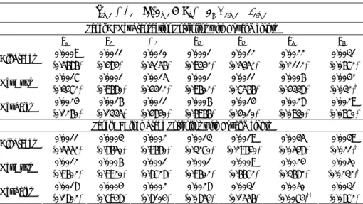
Table 1 shows the estimation results of the equally weighted portfolios from the traditional unconditional single-factor market model. Fundamentally, regarding net transaction portfolios from Panel A of Table 1, there are no significant abnormal returns in the month of trade (month 0) and over the following six months while there are negative abnormal returns at the sixth month for the net buy portfolio. Therefore, it seems that there are no abnormal profits for insider trading under the equally weighted insider portfolios. For the portfolios with block trades, the same findings as in Panel A result. Consequently, even for block trades, which are thought to significantly affect the price movements in the stock market, there are no traces of significant abnormal returns for insider trading except that there are still negative abnormal returns found in the later months.

Table 1. Estimation Results of Unconditional Single-Factor Market Model

1

' '

1, 1t 1 1( t 1 t) e 1, 1t 1, 1t

r ₊ =α +b F₊ ⊗Z +µ D ₊ +ε ₊

Panel A: Net Transaction Portfolios with Equal Weights

µ0 µ1 Μ2 µ3 µ4 µ5 µ6 0.0009 −0.0011 −0.0010 −0.0001 −0.0012 −0.0022 −0.0031 All Trades (0.5686) (0.484) (0.5156) (0.9442) (0.5352) (0.2112) (0.0672) −0.0017 −0.0001 −0.0015 −0.0001 −0.0011 −0.0006 −0.0042 Net Buys (0.3472) (0.9680) (0.4412) (0.9602) (0.7566) (0.4338) (0.032)* 0.0024 −0.0016 −0.0011 −0.0006 −0.0014 −0.0028 −0.0029 Net Sales (0.1260) (0.1335) (0.4840) (0.6966) (0.4010) (0.0930) (0.0970) Panel B: Block Trade Portfolios with Equal Weights

0.0011 −0.0003 −0.0002 −0.0013 −0.0019 −0.0035 −0.0039 All Trades (0.5552) (0.8650) (0.9680) (0.3270) (0.29840) (0.0548) (0.021)* 0.0012 0.0006 0.0001 0.0001 −0.0009 −0.0024 −0.0050 Net Buys (0.9602) (0.9920) (0.8728) (0.9602) (0.6672) (0.3682) (0.0232)* 0.0018 −0.0004 −0.0002 −0.0028 −0.0031 −0.0050 −0.0031 Net Sales (0.1802) (0.7948) (0.8104) (0.0854) (0.1556) (0.0074)** _(0.0872)

Note: μ0 represents the month of insider trades (month 0) and μ1 to μ6 represent the following six

months after month 0. p-values are reported in parentheses. ** and * represent significance levels of 0.01 and 0.05, respectively.

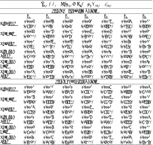
In order to examine whether or not the empirical results in Table 1 are robust, the conditional multi-factor model which takes information and risk factors into consideration is employed. Instead of using equally weighted portfolios, which are not appropriate in investment practice, the market value-weighted and ownership-weighted portfolios are formed to consider investment portfolios that conform to financial practice. Table 2 reports the estimation results of the market value-weighted portfolios in Panel A and ownership-weighted portfolios in Panel B using a conditional multi-factor model. It is found that there are no significant abnormal returns for the month of trade and the following months. Accordingly,

insider trading on the TWSE cannot create any significant extra profits. In order to determine whether the abnormal returns are present even after 6 months, the empirical results for an extension of the window size to 12 months are provided in Tables 3 and 4. Generally, the results are similar to those in Tables 1 and 2.

Table 2. Estimation Results of Conditional Multi-factor Model 1 , 1 1 , 1 ' 1 ' 1 1 1 , 1t+ = +b(Ft+ ⊗Zt)+ e1Dt+ + t+ r α µ ε

Panel A: Market Value Weights

µ0 µ1 µ2 µ3 µ4 µ5 µ6 0.0003 −0.0046 −0.0034 −0.0031 −0.0029 −0.0035 −0.0012 All Trades (0.7642) (0.246) (0.303) (0.3844) (0.3682) (0.2947) (0.6384) −0.0033 −0.0028 −0.0027 −0.0009 −0.0008 −0.0011 −0.0042 Net Buys (0.4122) (0.3844) (0.418) (0.6242) (0.617) (0.5156) (0.4592) −0.0002 −0.0049 −0.0048 −0.0041 −0.0021 −0.0060 0.0011 Net Sales (0.749) (0.2262) (0.197) (0.303) (0.4778) (0.095) (0.8026) −0.0005 −0.0035 −0.0035 −0.0045 −0.0050 −0.0026 −0.0004 All Block Trades (0.7114) (0.3628) (0.4122) (0.2802) (0.2112) (0.4354) (0.8572) 0.0001 −0.0025 −0.0016 −0.0004 −0.0014 −0.0008 −0.0050 Net Block Buys (0.968) (0.4966) (0.5824) (0.1032) (0.6528) (0.562) (0.4122) 0.0015 −0.0031 −0.0035 −0.0066 −0.0056 −0.0039 0.0016 Net Block Sales (0.9522) (0.4296) (0.4010) (0.1442) (0.1836) (0.3320) (0.9602) Panel B: Ownership Weights

0.0002 −0.0021 −0.0010 −0.0001 −0.0007 −0.0011 −0.0005 All Trades (0.8414) (0.5552) (0.6528) (0.7872) (0.7188) (0.5686) (0.7114) −0.0026 −0.0001 −0.0010 −0.0004 −0.0009 0.0001 −0.0021 Net Buys (0.4654) (0.8886) (0.6892) (0.7642) (0.7718) (0.7794) (0.4966) 0.0025 −0.0031 −0.0011 −0.0009 0.0001 −0.0023 0.0002 Net Sales (0.7794) (0.3954) (0.6242) (0.6384) (0.7872) (0.3954) (0.7871) 0.0010 −0.0016 0.0011 −0.0018 −0.0019 −0.0028 −0.0005 All Block Trades (0.968) (0.5962) (0.9362) (0.5686) (0.5552) (0.3898) (0.7262) −0.0004 −0.0006 0.0023 −0.0001 0.0000 −0.0017 −0.0022 Net Block Buys (0.7040) (0.7414) (0.9044) (0.9362) (0.9760) (0.5156) (0.4966) 0.0030 −0.0017 0.0004 −0.0034 −0.0029 −0.0045 −0.0001 Net Block Sales (0.6242) (0.5156) (0.9044) (0.3222) (0.3524) (0.2040) (0.8026) Note: μ0 represents the month of insider trades (month 0) and μ1 to μ6 represent the following six

months after month 0. p-values are reported in parentheses. ** and * represent the significance levels of 0.01 and 0.05, respectively.

The empirical results found in Tables 1 to 4 are not consistent with the findings in previous studies for other countries, such as Finnerty (1976a), Pope et al. (1990) and Seyhun (1988), who report that there are some significant abnormal returns associated with insider trading. However, our findings in the single-factor and multi-factor models are mostly consistent with those in Eckbo and Smith (1998). They claim that abnormal returns, largely an artifact of the single-factor model, are not found on the Oslo Stock Exchange using the multi-factor model.

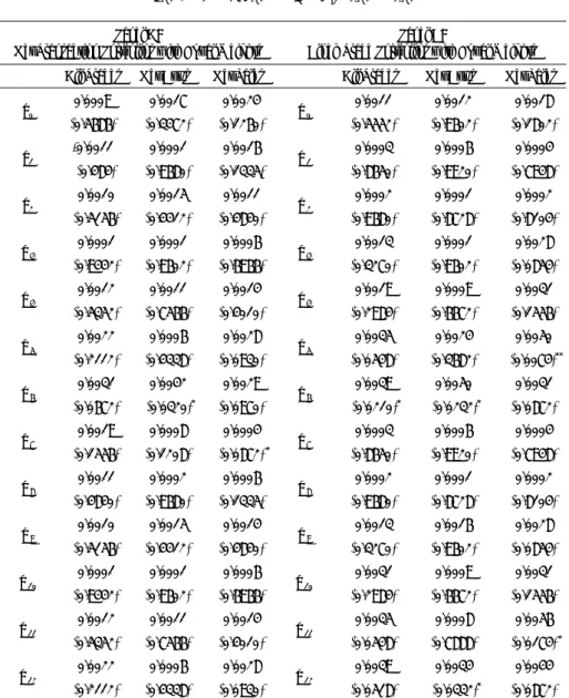
Table 3. Estimation Results of Unconditional Single-Factor Market Model When the Event Window is Reset to One Year

1

' '

1, 1t 1 1( t 1 t) e 1, 1t 1, 1t

r + =α +b F+ ⊗Z +µ D + +ε +

Panel A:

Net Transaction Portfolios with Equal Weights

Panel B:

Block Trade Portfolios with Equal Weights All Trades Net Buys Net Sales All Trades Net Buys Net Sales

0.0009 −0.0017 0.0024 0.0011 0.0012 0.0018 µ0 (0.5686) (0.3472) (0.1260) µ 0 (0.5552) (0.9602) (0.1802) -0.0011 −0.0001 −0.0016 −0.0003 0.0006 −0.0004 µ1 (0.484) (0.9680) (0.1335) µ 1 (0.8650) (0.9920) (0.7948) −0.0010 −0.0015 −0.0011 −0.0002 0.0001 −0.0002 µ2 (0.5156) (0.4412) (0.4840) µ 2 (0.9680) (0.8728) (0.8104) −0.0001 −0.0001 −0.0006 −0.0013 0.0001 −0.0028 µ 3 (0.9442) (0.9602) (0.6966) µ 3 (0.3270) (0.9602) (0.0854) −0.0012 −0.0011 −0.0014 −0.0019 −0.0009 −0.0031 µ 4 (0.5352) (0.7566) (0.4010) µ 4 (0.2984) (0.6672) (0.1556) −0.0022 −0.0006 −0.0028 −0.0035 −0.0024 −0.0050 µ 5 (0.2112) (0.4338) (0.0930) µ 5 (0.0548) (0.3682) (0.0074)** −0.0031 −0.0042 −0.0029 −0.0039 −0.0050 −0.0031 µ 6 (0.0672) (0.0320)* _(0.0970) µ 6 _(0.0210)* _(0.0232)* _(0.0872) −0.0019 −0.0008 −0.0004 −0.0003 0.0006 −0.0004 µ 7 (0.1556) (0.1208) (0.0872) * µ 7 _{(0.8650) (0.9920) (0.7948)} −0.0011 −0.0002 −0.0006 −0.0002 0.0001 −0.0002 µ 8 (0.4840) (0.9680) (0.1335) µ 8 (0.9680) (0.8728) (0.8104) −0.0010 −0.0015 −0.0014 −0.0013 0.0016 −0.0028 µ 9 (0.5156) (0.4412) (0.4840) µ 9 (0.3270) (0.9602) (0.0854) −0.0001 −0.0001 −0.0006 −0.0031 −0.0009 −0.0031 µ 10 (0.9442) (0.9602) (0.6966) µ 10 (0.2984) (0.6672) (0.1556) −0.0012 −0.0011 −0.0014 −0.0035 −0.0008 −0.0056 µ 11 (0.5352) (0.7566) (0.4010) µ 11 (0.0548) (0.7888) (0.0174) * −0.0022 −0.0006 −0.0028 −0.0039 −0.0034 −0.0044 µ 12 (0.2112) (0.4338) (0.0930) µ 12 (0.0518) (0.0332)* _(0.0872)

Note: μ0 represents the month of insider trades (month 0) and μ1 to μ12 represent the following

twelve months after month 0. p-values are reported in parentheses. ** and * represent the significance levels of 0.01 and 0.05, respectively.

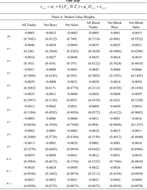
Table 4. Estimation Results of Conditional Multi-factor Model When the Event Window is Reset to One Year 1 , 1 1 , 1 ' 1 ' 1 1 1 , 1t+ = +b(Ft+ ⊗Zt)+ e1Dt+ + t+ r α µ ε

Panel A: Market Value Weights All Trades Net Buys Net Sales All Block

Trades Net Block Buys Net Block Sales 0.0003 −0.0033 −0.0002 −0.0005 0.0001 0.0015 µ0 (0.7642) (0.4122) (0.749) (0.7114) (0.968) (0.9522) −0.0046 −0.0028 −0.0049 −0.0035 −0.0025 −0.0031 µ 1 (0.246) (0.3844) (0.2262) (0.3628) (0.4966) (0.4296) −0.0034 −0.0027 −0.0048 −0.0035 −0.0016 −0.0035 µ 2 (0.303) (0.418) (0.197) (0.4122) (0.5824) (0.4010) −0.0031 −0.0009 −0.0041 −0.0045 −0.0004 −0.0066 µ 3 (0.3844) (0.6242) (0.303) (0.2802) (0.1032) (0.1442) −0.0029 −0.0008 −0.0021 −0.0050 −0.0014 −0.0056 µ 4 (0.3682) (0.617) (0.4778) (0.2112) (0.6528) (0.1836) −0.0035 −0.0011 −0.0060 −0.0026 −0.0008 −0.0039 µ 5 (0.2947) (0.5156) (0.095) (0.4354) (0.562) (0.3320) −0.0012 −0.0042 0.0011 −0.0004 −0.0050 0.0016 µ 6 (0.1384) (0.4592) (0.8026) (0.8572) (0.4122) (0.9602) −0.0003 0.0006 −0.0004 −0.0011 −0.0001 −0.0016 µ 7 (0.0650) (0.3920) (0.7948) (0.484) (0.9680) (0.1335) −0.0002 0.0001 −0.0002 −0.0010 −0.0015 −0.0011 µ 8 (0.2680) (0.5728) (0.8104) (0.5156) (0.4412) (0.4840) −0.0013 −0.0001 −0.0028 −0.0001 −0.0001 −0.0016 µ 9 (0.3270) (0.6602) (0.0854) (0.6442) (0.5602) (0.6966) −0.0019 −0.0049 −0.0031 −0.0012 −0.0011 −0.0024 µ 10 (0.2984) (0.6672) (0.1556) (0.5352) (0.7566) (0.4010) −0.0028 −0.0024 −0.0050 −0.0022 −0.0026 −0.0068 µ 11 (0.0548) (0.3682) (0.0074) (0.2112) (0.4338) (0.0930) −0.0031 −0.0052 −0.0031 −0.0031 −0.0042 −0.0049 µ 12 (0.0926) (0.0735) (0.0872) (0.0672) (0.0918) (0.0970) Note: µ0 represents the month of insider trades (month 0) and µ1 to µ12 represent the following twelve

months after month 0. p-values are reported in parentheses. ** and * represent the significance levels of 0.01 and 0.05, respectively.

Table 4. Estimation Results of Conditional Multi-factor Model When the Event Window is Reset to One Year (Continued)

1

' '

1, 1t 1 1( t 1 t) e 1, 1t 1, 1t

r ₊ =α +b F₊ ⊗Z +µ D ₊ +ε ₊

Panel B: Ownership Weights

All Trades Net Buys Net Sales All Block _Trades Net Block _Buys Net Block _Sales 0.0002 −0.0026 0.0025 0.0010 −0.0004 0.0030 µ0 (0.8414) (0.4654) (0.7794) (0.968) (0.7040) (0.6242) −0.0021 −0.0001 −0.0031 −0.0016 −0.0006 −0.0017 µ 1 (0.5552) (0.8886) (0.3954) (0.5962) (0.7414) (0.5156) −0.0010 −0.0010 −0.0011 0.0011 0.0023 0.0004 µ 2 (0.6528) (0.6892) (0.6242) (0.9362) (0.9044) (0.9044) −0.0001 −0.0004 −0.0009 −0.0018 −0.0001 −0.0034 µ 3 (0.7872) (0.7642) (0.6384) (0.5686) (0.9362) (0.3222) −0.0007 −0.0009 0.0001 −0.0019 0.0000 −0.0029 µ 4 (0.7188) (0.7718) (0.7872) (0.5552) (0.9760) (0.3524) −0.0011 0.0001 −0.0023 −0.0028 −0.0017 −0.0045 µ 5 (0.5686) (0.7794) (0.3954) (0.3898) (0.5156) (0.2040) −0.0005 −0.0021 0.0002 −0.0005 −0.0022 −0.0001 µ 6 (0.7114) (0.4966) (0.7871) (0.7262) (0.4966) (0.8026) −0.0016 −0.0006 −0.0017 −0.0046 −0.0028 −0.0049 µ 7 (0.5962) (0.7414) (0.5156) (0.2460) (0.3844) (0.2262) 0.0011 0.0023 0.0004 −0.0034 −0.0027 −0.0048 µ 8 (0.9362) (0.9044) (0.9044) (0.303) (0.418) (0.1970) −0.0018 −0.0001 −0.0034 −0.0039 −0.0009 −0.0024 µ 9 (0.5686) (0.9362) (0.3222) (0.3844) (0.6242) (0.4778) −0.0011 −0.0017 −0.0029 −0.0029 −0.0008 −0.0021 µ 10 (0.5552) (0.9760) (0.3524) (0.3682) (0.3030) (0.2882) −0.0028 −0.0047 −0.0045 −0.0035 −0.0011 −0.0060 µ 11 (0.3898) (0.5156) (0.2040) (0.2947) (0.5156) (0.0951) −0.0015 −0.0026 −0.0001 −0.0012 −0.0042 0.0011 µ 12 (0.7262) (0.4966) (0.8026) (0.6172) (0.4592) (0.6557) Note: μ0 represents the month of insider trades (month 0) and μ1 to μ12 represent the following

twelve months. p-values are reported in parentheses. ** and * represent the significance levels of 0.01 and 0.05, respectively.

3.2 Conditional Jensen’s alpha

Table 5 presents the GMM estimation results of the conditional Jensen’s alpha measures using 10 size-sorted decile portfolios of market value weights. Here, we use two types of Jensen’s alpha measures: one is estimated by time-varying betas, α , and the other is estimated by keeping betas fixed, α . Most of the portfolios *

show no significant measures under either type while there are only three significant alphas associated with the constant beta type. Since the time-varying beta measures accommodate the time-varying systematic risks in the stock market, which are much more reliable than constant beta type measures, there are no significant performances with size-sorted decile portfolios. This is consistent with findings in the multi-factor model.

Table 5. GMM Estimation Results of the Conditional Jensen’s α Measures for Decile Portfolios

' , 1 1 1_{p t} F_{t p}Z_t υ ₊ = ₊ −γ 1 , 1 , ' ' 1 , 1 , 1 , ( 1 1 )( ) 1 2pt+ = υ pt+υ pt+ κpZt −υ pt+rpt+ υ ' ' ' , 1 , 1 3_{p t} r_{p t p} ( _pZ_t) ( _pZ_t) υ ₊ = ₊ −α − γ κ ' ' , 1 , 1 . 1 ( 1_{p t t}, 2_{p t t}, 3_{p t} ) 0 Eυ ₊ Z υ ₊Z υ ₊ = αp α*p All Stocks −0.0107 (0.5816) −0.0105 (0.3607) Decile 1 −0.0017 (0.5162) 0.0082 (0.4033) Decile 2 −0.0101 (0.5741) −0.0117 (0.0342)* Decile 3 −0.0194 (0.6297) −0.0195 (0.1610) Decile 4 −0.0166 (0.6089) −0.0167 (0.1856) Decile 5 −0.0216 (0.6543) −0.0295 (0.1508) Decile 6 −0.0073 (0.5476) 0.1085 (0.0001)** Decile 7 _(0.6164) −0.0171 _(0.2425) −0.0234 Decile 8 _(0.6126) −0.0154 _(0.0159)−0.0228 * Decile 9 _(0.6674) −0.0271 _(0.3199) −0.0259 Decile 10 _(0.6654) −0.0241 _(0.1851) −0.0180

Note: αp represents Jensen’s α with time-varying betas and α*p represents Jensen’s α with constant betas.

Ten size-sorted decile portfolios are constructed based on beginning-of-month market values. Decile 1 contains the largest market value stocks while Decile 10 contains the smallest market value stocks. All portfolios are formed by market value weights. p-values are reported in parentheses. ** and * represent the significance levels of 0.01 and 0.05, respectively.

To explore more about the performances of distinct insider portfolios, we form portfolios according to firm characteristics. Table 6 reports the estimation results of conditional Jensen’s alpha measures using market-value weighted portfolios constructed with firm characteristics. There are no significant Jensen’s alpha

measures under time-varying beta measures while there are only three significant measures under constant beta measures. The significantly negative α for the small *

firm-sized portfolio is consistent with findings in Givoly and Palmon (1985) and Seyhun (1988) who find that abnormal returns tend to happen for small-sized firms.

Table 6. GMM Estimation Results of the Conditional Jensen’s α Measures for Firm Characteristics Portfolios of Market Value Weights

' , 1 1 1_{p t} F_{t p}Z_t υ ₊ = ₊ −γ ' ' , 1 , 1 , 1 , 1 , 1 2_{p t} ( 1_{p t} 1_{p t} )( _pZ_t) 1_{p t} r_{p t} υ ₊ = υ ₊υ ₊ κ −υ _{+ +} ' ' ' , 1 , 1 3_{p t} r_{p t p} ( _pZ_t) ( _pZ_t) υ ₊ = ₊ −α − γ κ ' ' , 1 , 1 . 1 ( 1_{p t t}, 2_{p t t}, 3_{p t} ) 0 Eυ ₊ Z υ ₊Z υ ₊ = αp α*p All Trades −0.0088 (0.5722) −0.0102 (0.1810) Net Buys −0.0102 (0.5842) −0.0124 (0.0953) Net Sells −0.0075 (0.5604) −0.0384 (0.2932) All Block Trades −0.0136

(0.5604)

0.0183 (0.0307)*

Net Block Buys −0.0145 (0.5958)

−0.0207 (0.0000)**

Net Block Sales −0.0126 (0.5806) −0.0149 (0.0539) Business Group −0.0061 (0.5502) 0.0318 (0.0881) Non-Business Group −0.0111 (0.5888) −0.0123 (0.1612) Large Firm Size −0.0073

(0.5610)

−0.0075 (0.2152) Medium Firm Size −0.0154

(0.6071)

−0.0147 (0.2517) Small Firm Size −0.0231

(0.6586)

−0.0223 (0.0236)*

High P/E Ratio −0.0092 (0.5681)

0.0091 (0.4377) Medium P/E Ratio −0.0099

(0.5743)

−0.0062 (0.2244) Low P/E Ratio −0.0148

(0.6033)

−0.0215 (0.2044)

Note: αprepresents Jensen’s α with time-varying betas and α*p represents Jensen’s α with constant betas.

All portfolios are formed by market value weights. p-values are reported in parentheses. ** and * represent the significance levels of 0.01 and 0.05, respectively.

In addition, the significantly negative α in the net block buy portfolio, also *

found in Eckbo and Smith (1998), may reflect that insiders purchase stocks for long-run performance, not for short-run performance. Table 7 shows estimation results for insider characteristic portfolios of ownership weights. The empirical

results in Table 7 are similar to those in Table 6. Therefore, on the TWSE, we cannot reject the hypothesis that there are no abnormal returns in insider trading.

Table 7. GMM Estimation Results of the Conditional Jensen’s α Measures for Firm Characteristics Portfolios of Ownership Weights

t p t t p F Z ' 1 1 , 1 γ υ + = + − 1 , 1 , ' ' 1 , 1 , 1 , ( 1 1 )( ) 1 2pt+ = υ pt+υ pt+ κpZt −υ pt+rpt+ υ ) ( ) ( 3 ' ' ' 1 , 1 ,t pt p p t p t p r α γ Z κ Z υ + = + − − 0 ) 3 , 2 , 1 ( . 1 ' 1 , ' 1 ,t+ t pt+ t pt+ = p Z Z Eυ υ υ αp α*p All Trades −0.0161 (0.6195) −0.0095 (0.3236) Net Buys −0.0185 (0.6315) −0.0170 (0.1947) Net Sells −0.0144 (0.6056) −0.0167 (0.2036) All Block Trades −0.0167

(0.6167)

−0.0745 (0.0000)**

Net Block Buys −0.0213 (0.6377)

−0.0273 (0.1755) Net Block Sales −0.0217

(0.6391) −0.0239 (0.1572) Business Group −0.0036 (0.0036) −0.0704 (0.1411) Non-Business Group −0.0199 (0.6400) 0.0211 (0.3267) Large Firm Size −0.0126

(0.5974)

−0.0078 (0.2898) Medium Firm Size −0.0145

(0.6003)

0.0312 (0.0705) Small Firm Size −0.0222

(0.6593)

−0.0188 (0.3573) High P/E Ratio −0.0176

(0.6285)

−0.0077 (0.1425) Medium P/E Ratio −0.0140

(0.6055)

−0.0148 (0.1421) Low P/E Ratio −0.0142

(0.5947)

−0.0095 (0.4046)

Note: αp represents Jensen’s α with time-varying betas and α*p represents Jensen’s α with constant betas.

All portfolios are formed by ownership weights. p-values are reported in parentheses. ** and * represent the significance levels of 0.01 and 0.05, respectively.

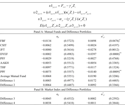
3.3 The performance difference between mutual fund managers and insiders In contrast to insider trading, managers of mutual funds make investment decisions by collecting information through their own analysts and various public information channels. Therefore, the performance comparisons between insider portfolios and mutual funds may reveal whether insiders with private information access are able to benefit more from their privileges or not. Eight mutual funds with

the best past five years performance during the sample period are selected according to the Mutual Fund Performance Evaluation Report published by the Securities Investment Trust and Consulting Association (SITCA) in Taiwan. These eight mutual funds are Fu Bon Fund (FBF), Citizen Securities Investment Trust Fund (CSIT), JF Taiwan Fund (JFT), The First Global Investment Trust Duo Yuan Equity Fund (DYEF), Prudential Financial Fund (PFF), ABN AMRO Kwang Hwa Fund (AAKH), Tung Hsin Fund (THF), and Prudential Pioneer Fund (PPF). Panel A of Table 8 presents the estimation results of conditional Jensen’s alpha measures for mutual funds and difference portfolios of market value weights and ownership weights. The difference portfolios are constructed by taking a long position in a mutual fund portfolio and a short position in insider trades. Hence, the difference portfolios may disclose direct performance comparisons between mutual funds and insiders. In addition, we compare the performances between market indices and difference portfolios of insider trading in Panel B of Table 8. This provides us with the opportunity to evaluate the information quality of insider trading and understand the trading motive behind insider activities. If insiders can make abnormal profits, then the information quality of insiders should at least be better than that of the market as a whole; otherwise, either the information quality of insiders is not good enough or the trading motive of the insiders is not limited to making abnormal profits.

As shown in Table 8, there are no significant conditional Jensen alpha measures for both types except for a few significant alpha measures of the constant beta type. Hence, mutual funds on the TWSE do not have any abnormal performances, which is also found in Ferson and Schadt (1996) and Eckbo and Smith (1998). In addition, there is weak evidence that mutual funds outperform insider portfolios. The insignificantly positive numbers in α and α in the two difference portfolios *

provide weak support for this finding. Accordingly, insider trading on the TWSE cannot gain any abnormal performances using privileged information. According to the results in Panel B of Table 8, we find that the information quality of insider trading is at least as good as that of the market as a whole since there are no significant differences between insider portfolios and market indices.

4. Conclusion

Given that insider trading is a long-standing attractive topic in financial research, this paper examines the performance of insider trading on the Taiwan Stock Exchange (TWSE), which can provide some understanding about insider trading in emerging markets. In addition to the traditional event study method, we adopt the conditional Jensen’s alpha approach proposed by Eckbo and Smith (1998). With the conditional Jensen’s alpha approach, we are able to consider effects of public information and risk factors and accommodate time-varying systematic risks. In addition, insiders’ trades are used to form portfolios under different financial criteria. We also compare the performances between insider portfolios, mutual funds, and market indices in order to gain insight into the likelihood that insiders with

privileged information perform better than managers of mutual funds that conduct intensive research on public information and expend great efforts to gather firm-specific information to beat the market.

The hypothesis that there are positive abnormal returns earned by insider trading is rejected in light of our empirical findings based on several weighting schemes and distinct portfolio construction methods. The conclusion is quite robust: the performance of insider trading is no better than the market indices. This may lead to a conjecture that insiders trading on the TWSE may not use privileged information to trade for short-term profits but rather for some other long-term objectives. Mutual funds weakly outperform insider trading yet do not enjoy any abnormal returns. Therefore, insiders may enjoy corporate control benefits from their ownership positions on the TWSE.

Table 8. GMM Estimation Results of the Conditional Jensen’s α Measures for Mutual Funds, Market Index, and Difference Portfolios

t p t t p F Z ' 1 1 , 1 γ υ + = + − 1 , 1 , ' ' 1 , 1 , 1 , ( 1 1 )( ) 1 2pt+ = υ pt+υ pt+ κpZt −υ pt+rpt+ υ ) ( ) ( 3 ' ' ' 1 , 1 ,t pt p p t p t p r α γ Z κ Z υ + = + − − 0 ) 3 , 2 , 1 ( . 1 ' 1 , ' 1 ,t+ t pt+ t pt+ = p Z Z Eυ υ υ

Panel A: Mutual Funds and Difference Portfolios

αp α*p FBF −0.0134 (0.5723) 0.0498 (0.0476)* CSIT −0.0062 (0.5499) −0.0024 (0.4197) JFT −0.0080 (0.5616) −0.0278 (0.0012) DYEF −0.0002 (0.4983) −0.0397 (0.0000)** PFF −0.0029 (0.5219) −0.0027 (0.4768) AAKH −0.0053 (0.5512) −0.0054 (0.3385) THF −0.0097 (0.5771) −0.0117 (0.1324) PPF −0.0075 (0.5557) −0.0140 (0.0009)**

Average Mutual Fund −0.0068 (0.5551) 0.0190 (0.3206)

Difference 1 0.0003 (0.4977) 0.0172 (0.4485)

Difference 2 0.0064 (0.4487) 0.0092 (0.3366)

Panel B: Market Index and Difference Portfolios

αp α*p

Difference 3 −0.0045 (0.4532) 0.0002 (0.2592)

Difference 4 0.0038 (0.5418) −0.0011 (0.3844) Note: αp represents Jensen’s α with time-varying betas and α*p represents Jensen’s α with constant betas.

Difference 1 and Difference 3 portfolios are calculated using market value weights while Difference 2 and Difference 4 portfolios are calculated using ownership weights. p-values are reported in parentheses. ** and * represent the significance levels of 0.01 and 0.05, respectively.

References

Baesel, J. B. and G. R. Stein, (1979), “The Value of Information: Inferences from the Profitability of Insider Trading,” Journal of Financial and Quantitative

Analysis, 14, 553-571.

Basu, S., (1983), “The Relationship between Earnings Yield, Market Value and Return for NYSE Common Stocks: Further Evidence,” Journal of Financial

Economics, 12, 129-157.

Eckbo, B. E. and D. C. Smith, (1998), “The Conditional Performance of Insider Trades,” Journal of Finance, 53, 467-498.

Evans, M. D., (1994), “Expected Returns, Time-Varying Risk and Risk Premia,”

Journal of Finance, 49, 655-679.

Ferson, W. E. and C. R. Harvey, (1993), “The Risk and Predictability of International Equity Market Returns,” Review of Financial Studies, 6, 527-566. Ferson, W. E. and R. W. Schadt, (1996), “Measuring Fund Strategy and Performance

in Changing Economic Conditions,” Journal of Finance, 51, 425-461.

Finnerty, J. E., (1976a), “Insiders’ Activity and Inside Information: A Multivariate Analysis,” Journal of Financial and Quantitative Analysis, 11, 205-216. Finnerty, J. E., (1976b), “Insiders and Market Efficiency,” Journal of Finance, 31,

1141-1148.

Givoly, D. and D. Palmon, (1985), “Insider Trading and the Exploitation of Insider Information: Some Empirical Evidence,” Journal of Business, 58, 69-87. Groenewold, N. and P. Fraser, (1997), “Share Price and Macroeconomic Factors,”

Journal of Business Finance & Accounting, 24, 1367-1383.

Hansen, L. P., (1982), “Large Sample Properties of the Generalized Method of Moments Estimators,” Econometrica, 50, 1029-1054.

Jaffe, J. J., (1974), “Special Information and Insider Trading,” Journal of Business, 47, 410-428.

Jensen, M. C., (1968), “Problems in Selection of Security Portfolios,” Journal of

Finance, 20, 389-419.

Kerr, H. S., (1980), “The Battle of Insider Trading vs. Market Efficiency,” Journal

of Portfolio Management, 6, 47-61.

Lee, M. H. and H. Bishara, (1989), “Recent Canadian Experience on the Profitability of Insider Trades,” The Financial Review, 24, 235-249.

Manne, H., (1966), Insider Trading and the Stock Market, New York: Free Press. Poon, S. and S. J. Taylor, (1991), “Macroeconomic Factor and UK Stock Market,”

Journal of Business Finance & Accounting, 18, 619-635.

Pope, P. F., R. C. Morris, and D. A. Peel, (1990), “Insider Trading: Some Evidence on Market Efficiency and Directors’ Share Dealings in Great Britain,” Journal

of Business Finance & Accounting, 17, 359-380.

Rozeff, M. S. and M. A. Zaman, (1988), “Market Efficiency and Insider Trading: New Evidence,” Journal of Business, 61, 25-44.

Seyhun, H. N., (1986), “Insiders’ Profits, Costs of Trading, and Market Efficiency,”

Journal of Financial Economics, 16, 189-212.

Journal of Business, 61, 1-24.

Seyhun, H. N., (1992), “Why Does Aggregate Insider Trading Predict Future Stock Returns?” The Quarterly Journal of Economics, 107, 1303-1331.

Trivoli, G. W., (1980), “How to Profit from Insider Trading Information,” Journal of