掃描鏈重新排列減少掃描移動功率架構在非指定的測試集合

(1)

國立交通大學

電子工程學系電子研究所碩士班

碩

碩士

士

士論

士

論

論文

論

文

掃描鏈重新排列減少掃描移動功率

架構在非

架構在非指

指

指定的測試集合

指

定的測試集合

Scan-Chain Reordering for Minimizing

Scan-Shift Power

Based on Non-Specified Test Cubes

研

研究

究

究生

究

生

生：

：

：吳育澤

吳育澤

指導教授

指導教授：

：

：趙家佐

趙家佐

趙家佐博士

博士

中

中華

華

華民

華

民

民國

國

國九十

國

九十七

九十

七

七年

年

年一

一

一月

月

(2)

掃描鏈重新排列減少掃描移動功率架構在非指定的測試集合

Scan-Chain Reordering for Minimizing Scan-Shift Power Based on

Non-Specified Test Cubes

研究生

研究生：

：

：吳育澤

吳育澤

Student：

：

：Yu-Ze Wu

指導教授

指導教授：

：

：趙家佐

趙家佐

Advisor：

：

：Chia-Tso Chao

：

國

國立

立

立交

交

交通

通

通大

大

大學

學

電子工程學系電子研究所碩士班

碩

碩士

士

士論

論

論文

論

文

A Thesis

Submitted to Department of Electronics Engineering & Institute of Electronics College of Electrical and Computer Engineering

National Chiao Tung University in Partial Fulfillment of the Requirements

for the Degree of Master

in

Electronics Engineering January 2008

Hsinchu, Taiwan, Republic of China 中華民國九十七年一月

(3)

i 掃描鏈重新排列減少掃描移動功率架構在非指定的測試集合掃描鏈重新排列減少掃描移動功率架構在非指定的測試集合掃描鏈重新排列減少掃描移動功率架構在非指定的測試集合 掃描鏈重新排列減少掃描移動功率架構在非指定的測試集合

學生

學生：

：

：吳育澤

：

吳育澤

吳育澤指導教授

吳育澤

指導教授：

指導教授

：

：趙家佐

趙家佐

趙家佐博士

博士

國立交通大學電子工程學系電子研究所碩士班

摘

摘要

要

這篇論文提出掃描元件的重新排列架構在非指定的測試集合

這篇論文提出掃描元件的重新排列架構在非指定的測試集合，

，

能保留測試圖案中不在乎位元的值用來減少在測試模式下所產生的

信號變動量

信號變動量。

。

。首先

首先

首先，

，

，我們提出以掃描元件反應值之間的關係性來引導

我們提出以掃描元件反應值之間的關係性來引導

重新排列

重新排列，

，

，並且用填值技術來減少掃描進的信號變動

，

並且用填值技術來減少掃描進的信號變動

並且用填值技術來減少掃描進的信號變動。

。

。接下來我們提

接下來我們提

出同時考慮掃描元件反應值和測試圖案之間的關係性來幫助排列並

且同時減少掃描進和出的信號變動

且同時減少掃描進和出的信號變動。

。

。一個反向的技術應用在此方法上

一個反向的技術應用在此方法上

進一步減少測試功率

進一步減少測試功率。

。

。除了功率導向的重新排列技術

除了功率導向的重新排列技術

除了功率導向的重新排列技術，

，

，我們最後提出

我們最後提出

同時考慮功率和繞線的方法

同時考慮功率和繞線的方法，

，

，在

，

在

在兩

在

兩

兩者間做取捨以達到減少違背時間限

兩

者間做取捨以達到減少違背時間限

制的情況

制的情況發生

發生

發生。

發生

。

。最後

最後

最後，

最後

，我們做一些實驗來論

，

我們做一些實驗來論

我們做一些實驗來論證

我們做一些實驗來論

證

證提出方法的有效性和優

提出方法的有效性和優

勢關於在減少掃描移動時所產生的信號變動

勢關於在減少掃描移動時所產生的信號變動。

。

。此

。

此

此外

此

外

外，

，

，關於同時考慮功

關於同時考慮功

率和繞線的

率和繞線的情況

情況

情況也透過實驗來做討論

也透過實驗來做討論

也透過實驗來做討論。

也透過實驗來做討論

。

(4)

ii

Scan-Chain Reordering for Minimizing Scan-Shift Power Based on Non-Specified Test Cubes

Student：

：

：Yu-Ze Wu

Advisor：

：

：Dr. Chia-Tso Chao

Department of electronics Engineering

Institute of Electronics

National Chiao Tung University

Abstract

This thesis proposes a scan-cell reordering scheme based on

unspecified test vectors to reduce the signal transitions during test mode

while preserving the don’t-care bits in the test patterns for a later

optimization. First, we introduce a method that uses response correlations

to guide the scan cell reordering and specify don’t care bits through a

pattern-filling technique to reduce scan-in transitions. Next, a proposed

scheme utilizes both response correlation and pattern correlation to

simultaneously minimize scan-out and scan-in transitions. A extension of

the scheme that reverse-combined technique applied to the method

further reduces test power. Except power-driven scan cell reordering

methodology, we last propose a methodology that takes the routing

overhead into consideration and derive a new ordering methodology

based on power and routing concerns. We can make a tradeoff between

power and routing to reduce timing violations. A series of experiments

(5)

iii

demonstrate the effectiveness and superiority of the proposed scheme on

reducing total scan-shift transitions. The effectiveness of the scheme

considering both power and routing overhead is discussed through

experiments as well.

(6)

iv

誌

誌謝

謝

時間過的很快，在交大兩年半的時間轉眼間就過去了。在這些日子中,雖然有遇到一些挫折，但很高興我有一群支持我、幫助我的人，讓我有可以去克服所遇到的困難。首先,我要感謝我的家人，在我遇到挫折的時候，他們總是給我鼓勵和支持，讓我在研究的旅途中可以無後顧之憂的走下去。另外，也非常感謝我的指導老師趙家佐教授在研究過程中的指點迷津，每當我遇到瓶頸時，它總能給我些建議，好讓我的研究之路能更順利。在日常生活方面，老師也會有透過聊天的方式談些個人經歷來給於諄諄教誨，人生規劃上也有一些建議。另外，也感謝實驗室的學弟啟銘、智為、偉勝在生活和研究上的交流。每當有程式方面的問題，偉勝總能給我蠻大的幫助，智為在工作站和 Tool 使用上的幫助，還有和啟銘討論研究方面的想法，這些都讓我在研究之路上更順遂。最後，我要感謝我的朋友們、勇全、育農、昭銘、子宗、聖偉、伯翰、亦琦、俊宇、宗翰等一些曾在研究所生涯中陪伴過我的朋友，有了你們，才讓我的研究所生活更多采多姿、更加順利。最後，再次向所有曾支持、關懷、幫助我的人，沒有你們就沒有現在的我。 2008 年吳育澤撰

(7)

v

Contests

摘摘摘 摘要要要 ... i 要 Abstract ... ii 誌誌誌 誌謝謝謝 ... iv 謝 Contents ... v

List of Tables ... vii

List of Figures ... viii

Chapter 1 Introduction ... 1

Chapter 2 Preliminaries ... 4

2.1 Scan-based Design ... 4

2.2 Test Power Challenge ... 6

Chapter 3 Power-driven Scan Cell Reordering ... 9

3.1 Previous Work ... 9

3.2Motivation ...12

3.3 Problem Formulation... ...14

3.4 Scan-cell Reordering Considering Only Response Correlation...16

3.4.1 Detailed Steps of Reordering Scheme ... 16

3.4.2 Experimental Results ... 20

3.5 Scan-cell Reordering Considering Both Response and Pattern Correlations ...24

3.5.1 Detailed Steps of Reordering Scheme ... 24

3.6 Scan-Cell Reordering Using Scan-data Inversion ...29

3.6.1 Detailed Steps of Reordering Scheme ... 29

Chapter 4 Scan Cell Reordering Considering Both Power and Routing Factors ...37

4.1 Detail Steps of Reordering Considering both Power and Routing Overhead ...37

4.1.1 Construct a Directed Multiple-Weight Graph Based on Correlations and Routing Overhead ... 38

(8)

vi

4.1.2 Find the Hamiltonian path with the minimum WTC ... 38

Chapter 5 Conclusions ...44

(9)

vii

List of Tables

Table 3-1 Response correlation of ISCAS benchmark s38584. ... 14

Table 3-2 Statistics of the circuits and their ATPG patterns ... 22

Table 3-3Comparisons of generated scan-shift transitions between RORC and [20] ... 23

Table 3-4 Different cases of pattern correlations between two adjacent cells. ... 25

Table 3-5 Comparisons of generated scan-shift transitions between RORC and ROBPR ... 30

Table 3-6 Different cases of inverse pattern correlations between two adjacent cells ... 32

Table 3-7 Comparisons of generated scan-shift transitions between ROBPR and SIRO ... 36

Table 4-1 Comparisons of scan-shift transitions on different optimization factor value and tool ordering [27] ... 41

Table 4-2 Comparisons of scan cahin length (um) on different optimization factor value and tool ordering [27] ... 42

(10)

viii

List of Figures

Figure 2-1 A scan design schematic ... 5

Figure 2-2 An example of scan-in, capture, and scan-out operation. ... 6

Figure 3-1 Graph construction based on deterministic sets ... 10

Figure 3-2 Different transition weight for test vectors and responses ... 11

Figure 3-3 Identifying the input and output of scan chain ... 12

Figure 3-4 Calculation of scan-in and scan-out WTC ... 17

Figure 3-5 Main steps of the proposed reordering scheme RORC ... 18

Figure 3-6 Construction of a response-correlation graph ... 19

Figure 3-7 Estimated WTCout of different scan-chain input/output ... 21

Figure 3-8 Main steps of the proposed reordering scheme ROBPR ... 24

Figure 3-9 Construction of the directed graph based on pattern and response correlations ... 26

Figure 3-10 The proposed algorithm for finding a Hamiltonian path with minimal WTCtotal... 28

Figure 3-11 Main steps of the proposed reordering scheme SIRO ... 31

Figure 3-12 Construction of the directed graph based on inverse and non-inverse correlation sets ... 33

Figure 3-13 Derive scan-in patterns in SIRO ... 34

Figure 3-14 Implement inverse techniques with traditional scan-chain architecture ... 35

Figure 4-1 Construction of the directed graph based on correlations and routing effects ... 39

Figure 4-2 The proposed algorithm for finding a Hamiltonian path optimizing power and routing overhead ... 40

Figure 4.3: The trends of transitions and chain length on different constrain factor and tool ordering ... 43

(11)

Chapter 1 Introduction

The scan design has been a widely used DFT technique which can guarantee high fault coverage for a complex design by enhancing its controllability and observability [1]. When using the scan design to shift test data, however, a large number of signal tran-sitions may occur along the scan paths, which induces even more signal trantran-sitions on the circuit-under-test (CUT). Therefore, with the scan design, the CUT will consume much more power in its test mode than that in its functional mode [2]. This excessive power consumption during the scan-based testing may result in physical damage or reli-ability degradation to the CUT, and in turn decreases the yield and product lifetime [3]. Another concern of this increased power is that significant IR Drop [4] causes good chips classified as fails and thus reduces the yield. As the number of scan cells keeps on growing in modern designs, this increasing power consumption has become one of the biggest barriers to effective the scan-based testing.

A common practice to lower the power consumption during scan-based testing is to reduce the number of scan cell’s signal transitions, which can be classified into the following three types: (1) the capture transition – generated by the same scan cell’s value difference between the scan-in pattern and the corresponding captured response, (2) the scan-out transition – generated by two adjacent scan cells’ value difference between their

(12)

Introduction 2 scan-out response, and (3) the scan-in transition – generated by two adjacent scan cells’ value difference between the scan-in patterns. The first transition type is associated with the capture power and the last two types are associated with the scan-shift power. In order to reduce the capture transitions, complex ATPGs [5][6][7][8][9] are proposed to generate test-pattern vectors which have a minimal hamming distance with their corresponding test-response vectors. Because the don’t care bits in their test cubes are fully specified for minimizing the capture transitions, the above ATPGs preclude the possibility for further test compaction or compression, and hence may result in a larger test set.

Methods are proposed to utilize the don’t-care bits to minimize the scan-in tran-sitions for a given test set [10][11][12][13]. [10] proposed a don’t-care-filling technique, named MT-fill, guaranteeing that the scan-in transitions generated by its filled patterns are minimized for the given test set. The methods in [11][12] reduced the test power as well as the test data volume based on build-in de-compression hardware. [13] added Xor gates or inverters along the scan paths to minimize the scan-in transitions. However, none of [10][11][12][13] considered the scan-out transitions simultaneously.

Another concept to reduce the scan-shift power is to partition the scan cells into mul-tiple groups and activate only one group at a time during the scan-shift cycles [14][15][16] [17][18][19]. It can limit the concurrent transitions in a small portion of the CUT. The partition methods require special control architectures to the scan designs, such as gated clocks [14], central control unit for each group’s clock signal [15][16], or specialized scan cells along with multiphase generator [18]. [19] further minimizes the capture power by only capturing responses for certain selected groups of scan cells. It requires a cus-tomized ATPG and discards a significant portion of responses.

Methods in [20][21] change the order of scan cells along the scan paths to minimize both scan-in and scan-out transitions based on given test patterns and responses. This scan-cell-reordering technique saves the scan-shift power, but sacrifices the opportunity

(13)

Introduction 3 of optimizing the wire length of scan paths during the APR stage [22][23]. In [24][25], re-ordering concerning the power and wire length is proposed. The methods is to minimize power as possible without violating the user-specific constrain of wire length. However, the existing scan-chain-reordering techniques [20][21][24][25] need to obtain the exact test patterns and responses in advance. As the result, no don’t-care bits can be utilized for a further reduction to scan-in transitions or test data volume, such as [10][11][12][13]. In this thesis, we attempt to develop a scan-cell-reordering scheme which can mini-mize the scan-out transitions while preserving the don’t-care bits in the test cubes for a later optimization of scan-in transitions using MT-fill [10]. To achieve this goal, we first need to predict the correlation between the response values before specifying don’t-care bits. This response correlation is an index to the possible scan-out transitions between scan cells and can be used as a guidance to the reordering process.Next, we consider the impact of scan-cell reordering on the result of MT-fill and simultaneously optimize the scan-in and scan-out transitions. Last, a scan-cell reordering considering power and routing factors is presented. We take scan chain length into consideration and trade off between power and routing length by user-specific coefficient of cost function consisting of power and routing factors. The experimental results demonstrate the effectiveness and the superiority of the proposed reordering scheme over a previous scan-cell reordering scheme [20].

(14)

Chapter 2 Preliminaries

2.1 Scan-based Design

To reduce the testing cost, we focus in design-for-test (DFT) techniques that aim at improving the testability. There are difficulties with the use of ad-hoc DFT methods. First, circuits are too large for manual inspection. Second, human testability experts are often hard to find, while the algorithmically generated testability measures are ap-proximate and do not always point to the source of the testability problem. Finally, even after DFT modifications are made, tests must be produced to enhance the fault coverage. Due to these reasons, the use of ad-hoc DFT is usually discouraged for larger circuits.

As the size and complexity of digital system grew, an alternative form of DFT, known as structured DFT. In structured DFT, extra logic and signals are added to the circuit so as to allow the test according to some predefined procedure. Apart from the normal functional mode, such a design will have one or more test modes. Commonly used structured methods are scan and built-in self test.

The main idea in scan design is to obtain control and observability for flips-flops. This is done by adding a test mode to the circuit such that when the circuit in this mode,

(15)

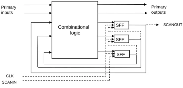
2.1 Scan-based Design 5 all flip-flops functionally form one or more shift registers. The inputs and outputs of these shift registers (also known as scan registers) are made into primary inputs (PIs) and primary outputs (POs). Thus, using the test mode, all flip-flops can be set to any desired states by shifting those logic states into the shift register. Similarly, the states of flip-flops are observed by shifting the contents of the scan register out. All flip-flops can be set or observed in a time that equals the number of flip-flops in the longest scan register. Figure 2.1 shows a complete scan design schematic.

Combinational logic SFF SFF SFF Primary inputs Primary outputs SCANOUT SCANIN CLK

Figure 2.1: A scan design schematic.

Generally, the test mode of scan-based design consist of three operation : scan-in operation, capture operation, scan-out operation. During testing, the scan-based design first has to specify flip-flop cells with the pattern values obtained from automatic test pattern generation (ATPG) process. Next, the design executes one-cycle logic simula-tion to update flip-flop values in capture operasimula-tion. Last, a serious of flip-flops response values is shifted out to be analyzed during scan-out operation. The scan-in and scan-out operation take several cycles which depend on the number of flips-flops of a scan-chain, but the capture operation takes one cycle.

(16)

2.2 Test Power Challenge 6 1011 1 1 1 0 1 1 1 0 1 1 Sout Sin 0 0 0 0 0 0

(a) scan-in operation

1 1 0 0 (b) capture operation Sin _S_out X X X X X X X X X X Sout Sin 1 1 0 1 1 1 (c) scan-out operation Combinational logic

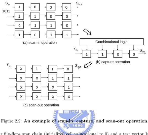
Figure 2.2: An example of scan-in, capture, and scan-out operation. a four flip-flops scan chain (initialized cell values equal to 0) and a test vector 1011 is given. During scan-in operation, it take four cycles to shift in the vector values to scan cells, and then new cell values are loaded from combinational logic in capture cycle. Last, responses are scan-out while the next pattern is shifted in simultaneously (Xs denote the values of next pattern) .

2.2 Test Power Challenge

Test power is a possible major engineering problem in the future of system-on-chip (SOC) development. As both the SoC designs and the deep-submicron geometry become prevalent, larger designs, tighter timing constrains, higher operating frequencies,

(17)

2.2 Test Power Challenge 7 and lower applied voltages all affect the power consumption systems of silicon devices. More precisely, these factors affect energy, average power, instantaneous power, and peak power, so some characteristics are defined.

• Energy: The total switching activity generated during test application, energy affects the battery lifetime during power up or periodic self-test of battery-operated devices.

• Average power: Average power is the total distribution of power over a time period. The ratio of energy to test time gives the average power. Elevated average power increases the thermal load that must be vented away from the device under test to prevent structural damage (hot spots) to the silicon, bonding wires, or packages. • Instantaneous power: Instantaneous power is the value of power consumed at

any given instant. Usually, it is defined as the power consumed right after the application of a synchronizing clock signal. Elevated instantaneous power might overload the power distribution systems of the silicon or package, causing brown-out.

• Peak power: The highest power value at any given instant, peak power determines the component’s thermal and electrical limits and system packaging requirements. If peal power exceeds a certain limit, designers can no longer guarantee that entire circuit will function correctly. In fact, the time window for defining peak power is related to the chip’s thermal capacity, and forcing this window to one clock period is sometimes just a simplifying assumption. For example, consider a circuit that has a peak power consumption during only one cycle but consumes power within the chip’s thermal capacity for all other cycles. In this case, the circuit is not damages, because the energy consumed-which corresponds to the peak power consumption time one cycle-will not be enough to elevate the temperature over

(18)

2.2 Test Power Challenge 8 the chip’s thermal capacity limit. To damage the chip, high power consumption must last for several cycles.

The scan-based design architecture are popular because of their low impact on per-formance and area. But these scan-based architecture are expensive because each test pattern requires a power-consuming shift operation to provide test patterns and evalu-ate test response. This phenomenon is well known in industry. To meet specified power limits during test and avoid system destruction, it is really important to reduce power dissipation during scan shifting.

(19)

Chapter 3 Power-driven Scan Cell Reordering

3.1 Previous Work

In this section, we introduce the previous work about scan cell reordering method-ology to reduce power [20]. The prerequisite is the deterministic sets including test patterns and corresponding responses. The idea of the methodology is to find a scan cell ordering which generates the minimum transitions during shifting operation. (scan − in and scan − out operations)

The steps are described as following:

• Collect a deterministic sets of test patterns and corresponding responses.

• Determine a scan cell chaining to minimize total bit differences of adjacent cells in patterns and responses .

• Determine a scan cell ordering to minimize generated transitions during scan-in and scan-out operations.

The data in the first step is obtained from ATPG tool that generate the patterns with non-specified bits. In the second step, finding a scan cell chaining with the minimal

(20)

3.1 Previous Work 10 FF1 FF2 FF3 FF4 scan-in scan-out V₁= 1 0 0 1 R₁= 0 1 0 0 V₂= 0 1 0 1 R₂= 0 0 1 0 V₃= 1 1 1 1 R₃= 1 0 1 1 V₄= 1 0 1 0 R₄= 1 0 0 1 FF1 FF2 FF3 FF4 6 2 3 4 5 ₅

Figure 3.1: Graph construction based on deterministic sets

bit differences represents the high probability to minimize transitions as low as possible. A complete graph is constructed based on the deterministic sets to help us find out the solution. In the graph, a vertex denotes a scan cell and the edge weight represents the total bit difference of adjacent vertices. Figure 3.1 shows the graph construction based on deterministic sets. In the figure, the test sequence is composed of four test vectors (V1 to V4) and four output responses (R1 to R4). The scan chain has four flip-flops,

hence scan vectors are four-bit long. The initial order of the scan cells in the scan chain is depicted on the figure. According to the above description, flip-flop 1, denoted FF1, corresponds to bit 1 in each scan vector, and so on.

Next, we calculate the total number of bit differences between each pair of scan flip-flops, which represents the number of transitions that may be generated in the corresponding portion of the scan chain by connecting these two flip-flops together. Calculating the total number of bit differences between each pair of flip-flops provides the following results: d(FF1, FF2) = 6, d(FF1,FF3) = 3, d(FF1,FF4) = 2, d(FF2, FF3) = 5, d(FF2,FF4) = 4, d(FF3, FF4) = 5.

To determine a scan cell chaining with the minimum cost, a greedy traveling salesman problem (TSP) is applied to find the solution. In the cases, the chaining of cells

(21)

FF1-3.1 Previous Work 11 FF4-FF2-FF3-FF1 is the final solution.

In the third step, the input and output of scan chain are identified. The transitions that bit differences generate during shift operation has dependency with its position of the scan chain. A novel method called weighted transition counts (WTC) had been proposed to calculate transitions [10].

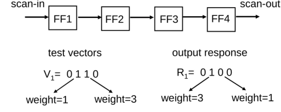
Figure 3.2 shows different transition weight for test vectors and responses. For test vectors, the bit difference of cell pair close to scan chain output generates more transi-tions because of passing through a long path during scan-in operation. The transition weight is increasing from the scan chain input. On the contrary, the weight of out re-sponse is decreasing from the scan chain input. As a result, the various combinations of input and output of scan chains cause different transition counts.

FF1 FF2 FF3 FF4

scan-in scan-out

test vectors output response

V₁= 0 1 1 0 R1= 0 1 0 0

weight=1 weight=3 weight=3 weight=1

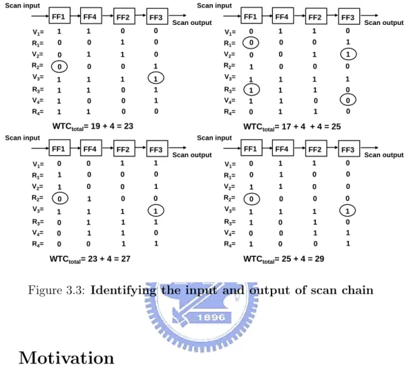
Figure 3.2: Different transition weight for test vectors and responses The third step tries and calculates the weighted transition counts for different cases to find the best ordering of scan cells with the minimum generated transitions during shift operation. Figure 3.3 describes the operation. Taking the chaining FF1-FF4-FF2-FF3 for example, the value of W T Ctotal is derived by calculating the weighted transition

counts of vectors and responses, respectively. Besides, the transitions generated due to the difference between the first bit of V3 and the last bit of R2 are also considered. The

(22)

3.2 Motivation 12 cells. FF1 FF4 FF2 FF3 Scan input Scan output V1= R1= V2= R2= V3= R3= V4= R4= 1 1 0 0 0 0 1 0 0 1 1 0 0 0 0 1 1 1 1 1 1 1 0 1 1 0 0 1 1 1 0 0 WTC_total= 19 + 4 = 23 FF1 FF4 FF2 FF3 Scan input Scan output V1= R1= V2= R2= V3= R3= V4= R4= 0 1 1 0 0 0 0 1 0 0 1 1 1 0 0 0 1 1 1 1 1 1 1 0 1 1 0 0 0 1 1 0 WTCtotal= 17 + 4 + 4 = 25 FF1 FF4 FF2 FF3 Scan input Scan output V1= R1= V2= R2= V3= R3= V4= R4= 0 0 1 1 1 0 0 0 1 0 0 1 0 1 0 0 1 1 1 1 0 1 1 1 0 1 1 0 0 0 1 1 WTC_total= 23 + 4 = 27 FF1 FF4 FF2 FF3 Scan input Scan output V1= R1= V2= R2= V3= R3= V4= R4= 0 1 1 0 0 1 0 0 1 1 0 0 0 0 0 0 1 1 1 1 1 0 1 0 0 0 1 1 1 0 0 1 WTC_total= 25 + 4 = 29

Figure 3.3: Identifying the input and output of scan chain

3.2 Motivation

During the scan-based testing, the total power consumption of the CUT is highly correlated with the total number of signal transitions on the scan cells [10]. In this thesis, we use the number of signal transitions on scan cells as the power model of the whole CUT. The proposed scan-cell-reordering scheme focuses on reducing the total scan-shift power, i.e., reducing the total scan-shift transitions. The capture power is not considered in the proposed scheme.

From the discussions in Chap. 1, the scan-in transitions can be minimized by wisely filling the don’t-care bits of a test set once the scan-cell order in the scan paths are given [10]. This reduction could be more significant as the percentage of don’t-care

(23)

3.2 Motivation 13 bits increases. Therefore, our scan-cell reordering scheme attempts to first minimize the scan-out transition count without specifying the care bits, leaving the don’t-care bits for a later minimization of scan-in transition, such as MT-fill [10]. However, before specifying the don’t-care bits, the value of some responses may not be obtainable, implying that no explicit information of scan-out transitions can be used during the scan-cell reordering process.

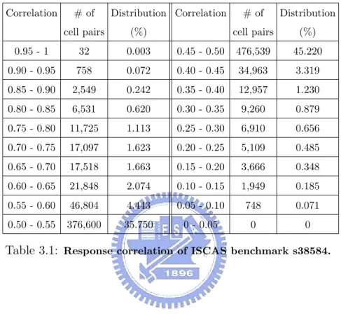
We use a simple experiment (reported in Table 3.1) to show that certain pairs of scan cells tend to have the same response value in most cases of the random don’t-care filling. Thus the reordering scheme can avoid the possible scan-out transitions by connecting those correlated pairs of scan cells next to each other. We first define this tendency between two scan cells as the response correlation, which is the probability that the two scan cells have the same response value by a random fill of don’t-care bits. In the experiment, we use a commercial tool [26] to generate stuck-at-fault patterns with don’t-care bits. We then collect the statistic of the response correla-tion between any two scan cells by randomly filling the don’t-care bits and simulating the corresponding responses for 1-million times. Table 3.1 lists the range of response correlations (Columns 1 and 4), the number of scan-cell pairs whose sampled response correlation falls in the range (Columns 2 and 5), and its corresponding percentage to the total scan-cell pairs (Columns 3 and 6), for the largest ISCAS benchmark circuit s38584. As the results show, while majority of the scan-cell pairs have a response correlation around 0.5, still 21595 scan-cell pairs (2%) have a response correlation higher than 0.75. Those 21595 scan-cell pairs could form a fair-sized solution space when reordering the 1452 scan cells in s38584. This experimental result indicates that, even without spec-ifying the don’t-care bits, the response correlations are not purely random. The same trend can be observed on other ISCAS and ITC benchmark circuits as well.

(24)

3.3 Problem Formulation 14

Correlation # of Distribution Correlation # of Distribution

cell pairs (%) cell pairs (%)

0.95 - 1 32 0.003 0.45 - 0.50 476,539 45.220 0.90 - 0.95 758 0.072 0.40 - 0.45 34,963 3.319 0.85 - 0.90 2,549 0.242 0.35 - 0.40 12,957 1.230 0.80 - 0.85 6,531 0.620 0.30 - 0.35 9,260 0.879 0.75 - 0.80 11,725 1.113 0.25 - 0.30 6,910 0.656 0.70 - 0.75 17,097 1.623 0.20 - 0.25 5,109 0.485 0.65 - 0.70 17,518 1.663 0.15 - 0.20 3,666 0.348 0.60 - 0.65 21,848 2.074 0.10 - 0.15 1,949 0.185 0.55 - 0.60 46,804 4.443 0.05 - 0.10 748 0.071 0.50 - 0.55 376,600 35.750 0 - 0.05 0 0

Table 3.1: Response correlation of ISCAS benchmark s38584.

3.3 Problem Formulation

The problem of the scan-cell reordering for scan-shift power reduction is first defined as follows:

Input:

• A circuit under test with scan cells inserted, and • ATPG test patterns with don’t care bits (X’s). Output:

(25)

3.3 Problem Formulation 15 • Test patterns with all don’t-care bits specified by MT-Fill based on the derived

cell ordering. Objective:

• Generate the minimum number of scan-shift transitions for the given test patterns. The proposed scan-cell-reordering scheme only discuss the situation of one scan chain in a design. However, the concept of the proposed reordering scheme could be extended to multiple-scan-chain architectures as well.

Given a test pattern and the scan-cell order for the scan chain, we can use the weighted transition count (WTC) [10] to calculate the number of scan-in and scan-out transitions. The WTC considers not only the value difference between the patterns or responses of two adjacent scan cells, but also the number of transitions that this value difference generates during the scan shift cycles. Equation 3.1 and 3.2 define the W T Cin(i) and W T Cout(i) to calculate the scan-in transitions and scan-out transitions

generated by the ith pattern, respectively.

W T Cin(i) = s−1 X j=0 P D(j) × WP D(j) (3.1) W T Cout(i) = s−1 X j=0 RD(j) × WRD(j) (3.2)

In equation 3.1 and 3.2, s denotes the total number of scan cells; P D(j) (RD(j)) denotes the value difference between the scan-in pattern (scan-out response) of the jth cell and the j + 1 cell; WP D(j) denotes the number of scan-in transitions generated by

the pattern-value difference P D(j) when shifting in the corresponding pattern values from the scan input to the j + 1 cell; WRD(j) denotes the number of scan-out transitions

generated by the response-value difference RD(j) when shifting out the responses from the j cell to the scan chain output.

(26)

3.4 Scan-cell Reordering Considering Only Response Correlation 16 In the WTC calculation, WP D(j) = j, implying that a pattern-value difference can

generate more scan-in transitions if this value difference occurs closer to the scan-chain output. On the contrary, WRD(j) = s − 1 − j, implying that a response-value difference

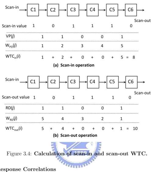
can generate more out transitions if this value difference occurs closer to the scan-chain input. Figure 3.4 shows an example of the WTC computation on a 6-cell scan chain, assuming that three value differences occur between cells (C1, C2) , (C2, C3), and

(C5, C6) for both the test pattern and its response.

Equation 3.3 calculates the total number of transitions, W T Ctotal, generated by a

given test set with m test patterns.

W T Ctotal = m

X

i=1

[W T Cin(i) + W T Cout(i)] (3.3)

3.4 Scan-cell Reordering Considering Only Response

Correlation

3.4.1 Detailed Steps of Reordering Scheme

We introduce a scan-cell reordering scheme, named RORC (ReOrdering considering Response Correlation), which first reduces the scan-out transitions by minimizing the response correlations while preserving all don’t-care bits in the test patterns. Then, the scan-in transitions are further minimized by specifying the don’t-care bits with MT-fill. Figure 3.5 shows the flow of RORC, which consists of five main steps. The detail of each step is described in the following subsections.

(27)

3.4 Scan-cell Reordering Considering Only Response Correlation 17 C1 C2 C3 C4 C5 C6 Scan-in value 1 0 1 1 1 0 W_PD(j) 1 2 3 4 5 WTC_in(i) _{1 + 2 + 0 + 0 + 5 = 8} C1 C2 C3 C4 C5 C6 Scan-out value 1 0 1 1 1 0 W_RD(j) 5 4 3 2 1 5 + 4 + 0 + 0 + 1 = 10 VP(j) _{1 1 0 0} ₁ 1 1 0 0 1 (a) Scan-in operation

(b) Scan-out operation RD(j) Scan-in Scan-out Scan-in Scan-out WTC_out(i)

Figure 3.4: Calculation of scan-in and scan-out WTC. Obtain Response Correlations

A simulation-based method is applied to sample the response correlations between each pair of scan cells. However, the filling of don’t-care bits in RORC is not purely ran-dom since the MT-fill technique will be applied later in RORC. Therefore, in this step, we randomly generate the scan-cell ordering multiple times, specify don’t-care bits using MT-fill based on each generated scan-cell ordering, and then collect the response corre-lations by simulating the filled patterns. The number of random-generated cell orderings used in simulation will determine the accuracy of the sampled response correlations. We use the following empirical equation to determine this number of random-generated cell

(28)

3.4 Scan-cell Reordering Considering Only Response Correlation 18

Step 1: Obtain the response correlations

Step 2: Construct the response-correlation graph based on the sampled response correlations

Step 3: Find a maximal Hamiltonian cycle on the response-correlation graph Step 4: Determine the cell ordering with minimum WTC by breaking the Hamil-tonian cycle

Step 5: Apply the MT-Fill to specify the don’t-care bits of test patterns based on the derived cell ordering

Figure 3.5: Main steps of the proposed reordering scheme RORC. orderings.

Simulation T imes = (G Counts/50) × P Counts, (3.4) where G Counts and P Counts denote the circuit gate count and the number of given test patterns, respectively.

Construct the Correlation Graph

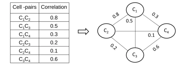
After obtaining the response correlations, we construct a non-directed graph, named response-correlation graph, in which a vertex represents a scan cell and the weight of each edge represents the response correlation between the adjacent vertices. Because any pair of scan cells could be placed next to each other, the response-correlation graph is a complete graph. Figure 3.6 shows an example of constructing a response-correlation graph with four scan cells.

(29)

Cell -pairs Correlation

C₁C₂ 0.8 C₁C₃ 0.5 C₁C₄ 0.3 C₂C₃ 0.2 C₂C₄ 0.1 C₃C₄ 0.6

C

₁

C

₂

C

4

C

₃ 0.8 0.3 0.2 0.6 0.5 0.1

Figure 3.6: Construction of a response-correlation graph. Find a Maximal Hamiltonian Cycle

A higher response correlation between two scan cells implies a lower probability that a response-value difference occurs between the two cells. Based on this concept, the maximum Hamiltonian cycle on the response-correlation graph implies a scan-cell ordering on which the number of value differences generated between adjacent cells is statistically minimum. Finding the maximum Hamiltonian cycle is known as the trav-eling salesman problem (TSP), which is NP-complete. We use a greedy TSP algorithm, which orders one vertex at a time to form the cycle. The selection criteria for the new ordered vertex is to find the vertex which has the maximum weight with the previous ordered vertex. In addition, we select the first N largest edges as the initial searching points and report the best result out of these N trials, where N denotes the total number of scan cells. The time complexity of this algorithm is Q(N3

). Determine Cell Ordering with Minimal WTC

In the previous step, we obtained a maximal Hamiltonian cycle on the response-correlation graph so that the number of potential response-value differences between adjacent cells can be minimized. However, to minimize the W T Cout, we need to

(30)

con-3.4 Scan-cell Reordering Considering Only Response Correlation 20 sider not only the number of response-value differences but also the positions of those value differences in the cell ordering (as discussed in Section 3.3). In Step 4, we break the given maximal Hamiltonian cycle into a Hamiltonian path, which forms the final scan-cell ordering. The breaking of the Hamiltonian cycle will affect the positions of the response-value differences and, in turn, affect the W T Cout. Here, we estimate the

W T Cout generated by each possible breaking of the given Hamiltonian cycle and use the

breaking with the minimum W T Cout to form the final cell ordering.

The estimated W T Cout here is obtained by replacing the RD(j) in Equation 3.2

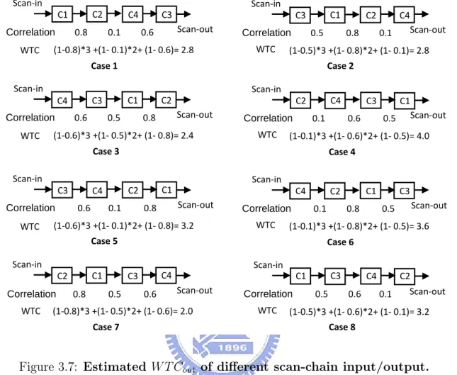
with 1 minus the response correlation between cell j and j +1. For example, the maximal Hamiltonian cycle in Figure 3.6 is C1-C2-C4-C3-C1. Figure 3.7 shows the estimated

W T Cout for all eight cases of the possible cycle breaking. The final cell ordering of the

scan chain is C2-C1-C3-C4.

Apply MT-Fill to Specify Don’t-care Bits

After the scan-cell ordering is decided in the previous step, we apply the MT-fill technique to fill the don’t-care bits of the test patterns so that the scan-in transitions based on the scan-cell ordering can be minimized. The rule of MT-fill is that a don’t-care bit is filled with the value of the first encountered specified bit when traversing from the don’t-care bit toward the scan-chain output. Refer to [10] for more details of MT-fill.

3.4.2 Experimental Results

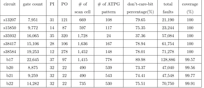
We conduct experiments on nine ISCAS and ITC benchmark circuits. Table 3.2 first shows the statistics of the benchmark circuits and their ATPG patterns generated by [26].

The following experiment compares RORC with another scan-cell reordering scheme presented in [20], which requires fully-specified test patterns before the reorder-ing. Since RORC applies MT-fill to minimize the scan-in transitions, we apply MT-fill

(31)

3.4 Scan-cell Reordering Considering Only Response Correlation 21 (1-0.8)*3 +(1- 0.1)*2+ (1- 0.6)= 2.8 Scan-out Correlation 0.8 0.1 0.6 WTC Case 1 Scan-in C1 C2 C4 C3 (1-0.5)*3 +(1- 0.8)*2+ (1- 0.1)= 2.8 Scan-out Correlation 0.5 0.8 0.1 WTC Case 2 Scan-in C3 C1 C2 C4 (1-0.6)*3 +(1- 0.5)*2+ (1- 0.8)= 2.4 Scan-out Correlation 0.6 0.5 0.8 WTC Case 3 Scan-in C4 C3 C1 C2 (1-0.1)*3 +(1- 0.6)*2+ (1- 0.5)= 4.0 Scan-out Correlation 0.1 0.6 0.5 WTC Case 4 Scan-in C2 C4 C3 C1 (1-0.6)*3 +(1- 0.1)*2+ (1- 0.8)= 3.2 Scan-out Correlation 0.6 0.1 0.8 WTC Case 5 Scan-in C3 C4 C2 C1 (1-0.1)*3 +(1- 0.8)*2+ (1- 0.5)= 3.6 Scan-out Correlation 0.1 0.8 0.5 WTC Case 6 Scan-in C4 C2 C1 C3 (1-0.8)*3 +(1- 0.5)*2+ (1- 0.6)= 2.0 Scan-out Correlation 0.8 0.5 0.6 WTC Case 7 Scan-in C2 C1 C3 C4 (1-0.5)*3 +(1- 0.6)*2+ (1- 0.1)= 3.2 Scan-out Correlation 0.5 0.6 0.1 WTC Case 8 Scan-in C1 C3 C4 C2

Figure 3.7: Estimated W T Cout of different scan-chain input/output.

for [20] as well. In the following experiment of [20], we first randomly generate an initial scan-cell ordering and specify the don’t-care bits using MT-fill according to that initial ordering. Then the reordering scheme in [20] is applied to obtain the final scan-cell ordering based on the filled patterns. We repeat the above steps 100 times and report the best results for [20]. Also, we use the same TSP algorithm in both RORC and [20] to make a fair comparison.

In Table 3.3, Columns 3, 4, and 5 list the numbers of scan-in transitions, scan-out transitions, total scan-shift transitions, respectively. Column 6 lists the peak number of scan-shift transitions at a single scan-shift cycle. Column 7 lists the runtime in seconds. The results show that RORC can outperform [20] with an average 43.28%

(32)

circuit gate count PI PO # of # of ATPG don’t-care-bit total coverage scan cell pattern percentage(%) faults (%)

s13207 7,951 31 121 669 108 79.65 21,190 100 s15850 9,772 14 87 597 117 75.35 23,244 100 s35932 16,065 35 320 1,728 24 37.36 57,084 100 s38417 15,106 28 106 1,636 167 78.94 61,754 100 s38584 19,253 12 278 1,452 148 78.01 71,278 100 b17 22,645 37 97 1,415 778 89.98 128,886 99.57 b20 8,875 32 22 490 539 73.37 47,040 99.56 b21 9,259 32 22 490 543 74.41 47,548 99.77 b22 14,282 32 22 735 530 75.51 70,750 99.91

Table 3.2: Statistics of the circuits and their ATPG patterns.

and 49.50% reduction to the number of scan-in transitions and scan-out transitions, respectively. The reduction to scan-in transitions first demonstrates the advantages of preserving don’t-care bits for later minimization. Also, the reduction to scan-out transitions demonstrates the effectiveness of using sampled response correlations to guide the reordering process. The reduction to peak transitions is a byproduct of the reduction to total scan-shift transitions. Note that the result reported for [20] is selected from 100 trials of random initial cell ordering. It implies that, even with MT-fill, specifying all don’t-care bits before reordering will significantly decrease the opportunity in minimizing scan-shift transitions later on and, in turn, lead to a local optimum.

RORC generates a lower number of total scan-shift transitions than [20] in all circuits but s35932. This exception may attribute to its low don’t-care-bit percentage of 37.36%. From our internal experiments, we found that a cell ordering will affect the results of the MT-fill more significantly when the don’t-care-bit percentage is lower. This finding further motivates us to develop a cell reordering scheme which can also consider the impact of a scan-cell ordering on the scan-in transitions generated by the

(33)

circuit method scan-in scan-out total peak runtime

trans. trans. trans. trans. (sec)

[17] 3,951,373 4,188,819 8,140,192 289 400 s13207 RORC 1,312,934 2,847,104 4,160,038 233 45 improv. 66.77 % 32.03 % 48.90 % 19.38% -[17] 2,800,025 4,904,948 7,704,973 277 300 s15850 RORC 1,497,065 2,157,662 3,654,727 211 49 improv. 46.53 % 56.01% 52.57 % 23.83% -[17] 4,543,209 4,934,478 9,477,687 525 3,000 s35932 RORC 5,388,270 4,363,125 9,751,395 680 120 improv. -18.60 % 11.58 % -2.89 % -29.52% -[17] 29,942,845 58,416,311 88,359,156 713 4,100 s38417 RORC 11,453,864 27,547,170 39,001,034 529 666 improv. 61.75 % 52.84 % 55.86 % 25.81% -[17] 22,827,002 41,743,137 64,570,139 714 3,100 s38584 RORC 12,489,481 27,615,042 40,104,523 694 616 improv. 45.29 % 33.85% 37.89 % 2.80% -[17] 95,302,661 230,963,547 326,266,208 700 6,200 b17 RORC 24,619,742 41,550,664 66,170,406 570 3,760 improv. 74.17 % 82.01% 79.72 % 18.57% -[17] 7,680,415 12,332,467 20,012,882 237 500 b20 RORC 4,823,088 4,662,118 9,485,206 171 160 improv. 37.20 % 62.20 % 52.60 % 27.85% -[17] 7,351,208 11,834,023 19,185,231 229 600 b21 RORC 4,546,521 4,590,188 9,136,709 205 177 improv. 38.15 % 61.21% 52.38 % 10.48% -[17] 17,200,814 23,447,118 40,647,932 362 1,200 b22 RORC 9,997,996 10,844,186 20,842,182 276 587 improv. 41.87 % 53.75 % 48.73 % 23.76% -Ave. improv. 43.68 % 49.50 % 47.30% 13.66%

(34)

3.5 Scan-cell Reordering Considering Both Response and Pattern

Correlations 24

MT-fill patterns.

3.5 Scan-cell Reordering Considering Both Response

and Pattern Correlations

3.5.1 Detailed Steps of Reordering Scheme

RORC reduces scan-out transitions by minimizing the response correlations between adjacent cells. It ignores the impact of the cell ordering on the number of scan-in transitions resulted from the MT-fill patterns. In this section, we introduce another scan-cell reordering scheme, named ROBPR (ReOrdering considering Both Pattern and Response correlation), which can simultaneously optimize the pattern correlations and response correlations during the reordering process. Figure 3.8 shows the flow of ROBPR consisting of four main steps. The details of steps 1-3 are described in the following subsections. The detail of step 4 is the same as the step 5 in RORC and hence omitted in this section.

Step 1: Collect pattern and response correlations

Step 2: Construct a directed multiple-weight graph based on the collected pattern and response correlations

Step 3: Find the Hamiltonian path with the minimum WTC

Step 4: Apply the MT-Fill to specify the don’t-care bits based on the derived cell ordering

(35)

Correlations 25

Obtain Pattern and Response Correlations

In order to measure the impact of a cell ordering on the number of scan-in transitions, we first defscan-ine the pattern correlation between cell i and cell j as the probability that the pattern values on these two cells are the same when the output of cell i is connected to the input of cell j. Note that this pattern correlation is dependent on the order of cells. For a test pattern k, Table 3.4 considers each combination of pattern values between cell i and cell j, and lists its corresponding pattern correlation after MT-fill (denoted as P Ck(i, j)).

case value of cell i value of cell j P Ck(i, j)

1 0 0 1 2 0 1 0 3 0 X S0/(S0+ S1) 4 1 0 0 5 1 1 1 6 1 X S1/(S0+ S1) 7 X 0 1 8 X 1 1 9 X X 1

Table 3.4: Different cases of pattern correlations between two adjacent cells.

In cases 1, 2, 4, and 5, both values of cell i and j are specified bits and hence their pattern correlations can be determined immediately for test pattern k. In cases 7, 8, and 9, a don’t-care bit are placed prior to a specified bit and hence the don’t-care bit will be filled with the same value as the specified bit. In cases 3 and 6, a specified bit is placed prior to a don’t-care bit. Hence, the value of this don’t-care bit cannot be derived immediately and has to be determined by its first encountered specified bit when traversing toward the scan-chain output. We use S0/(S0+ S1) (S1/(S0+ S1)) to

(36)

Correlations 26

S1 denote the total numbers of specified 1s and 0s in the test pattern, respectively.

After calculating the P Ck(i, j) for each pattern k, the pattern correlation between

cell i and cell j for the entire test set can be obtained by averaging the P Ck(i, j) for

each pattern k.

As to the response correlations, we use the same simulation-based method de-scribed in the Sec. 3.4.1 to estimate them.

Construct the Directed Correlation Graph

The correlation graph constructed in ROBPR is a revised version of the correlation graph in Sec. 3.4.1. First, this correlation graph is directed. Second, an edge in this correlation graph has two weights (Wp, Wr), where Wp and Wr represent the pattern

correlation and response correlation, respectively. Figure 3.9 shows an example of con-structing such a directed correlation graph given the pattern and response correlations between three scan cells.

Cell pairs Pattern correlation Response correlation C₁C₂ 0.5 0.8 C₁C₃ 0.2 0.5 C₂C₁ 0.1 0.8 C₂C₃ 0.4 0.2 C₃C₁ 0.6 0.5 C₃C₂ 0.1 0.2 C₁ C₂ C₃ (0.5 , 0.8 ) (0.1 , 0.8 ) (0_.2 , 0 .5₎ (0 .6 , 0 .5₎ (0.4, 0.2) (0.1, 0.2)

Figure 3.9: Construction of the directed graph based on pattern and response correlations.

(37)

Correlations 27

Find the Hamiltonian Path with Minimal WTC

Unlike RORC which finds a Hamiltonian cycle first and then breaks the Hamil-tonian cycle to obtain a HamilHamil-tonian path with minimal estimated W T Cout, ROBPR

uses an integrated algorithm to directly obtain the Hamiltonian path with minimal esti-mated W T Ctotal on the correlation graph. Figure 3.10 shows the proposed greedy-based

algorithm, which also ordered one new vertex at a time to form such a Hamiltonian path.

When adding the nth non-ordered vertex Vnon for the Hamiltonian path, this

algorithm uses a cost function Cost(Vlast, Vnon, n) to measure the impact of the

new-added edge (Vlast, Vnon) on W T Ctotal, which is defined in Equation 3.3. In the definition

of Cost(Vi, Vj, n) in Figure 3.10, the Wp(Vi, Vj) (Wr(Vi, Vj)) actually represents the

prob-ability that a pattern-value (response-value) difference occurs between Vi and Vj. The n

in the cost function actually represents the WP D(n) described in the WTC equation 3.1.

The N − 1 − n in the cost function actually represents the WRD(n) described in the

WTC equation 3.2.

This cost function will guide the algorithm to emphasize more on the response correlation in the beginning of the ordering process and then gradually move its emphasis to the pattern correlation in the later stage of the reordering process, which exactly reflects the WTC definition in Equations 3.1 and 3.2.

3.5.2 Experimental Results

We conduct experiments for ROBPR on the same benchmark circuits and test pat-terns as in Sec. 3.4.2. Table 3.5 compares the results of ROBPR with the results of RORC, which considers only the response correlation during the reordering. The ex-perimental results show that, in average, ROBPR can generate 33.87% less scan-in transitions but only 5.01% more scan-out transitions compared to RORC. This

(38)

signif-3.5 Scan-cell Reordering Considering Both Response and Pattern

Correlations 28

1 #define

2 Wp(Vi, Vj) : the pattern correlation of edge (Vi, Vj)

3 Wr(Vi, Vj) : the response correlation of edge (Vi, Vj)

4 Wp(Vi, Vj) : 1 − Wp(Vi, Vj)

5 Wr(Vi, Vj) : 1 − Wr(Vi, Vj)

6 Cost(Vi, Vj, n) : Wp(Vi, Vj) × n + Wr(Vi, Vj) × (N − 1 − n)

7 begin

8 N ← # of cells ; n ← 1 ;

9 M in l ← a list of N edges having the minimum (Wp+ Wr×(N -1));

10 for each directed edge e(Vi, Vj) of M in l

11 V1st←V_i, V_2nd←V_j, V_last←V_2nd; 12 while non-ordered V

13 costmin← ∞; n ← (n + 1) ; 14 for each non-ordered Vnon

15 if (Cost(Vlast, Vnon, n) < costmin)

16 costmin←Cost(V_last, V_non, n) ; 17 Vnext ←V_non ; 18 endif 19 endfor 20 Vlast←Vnext 21 endwhile 22 endfor 23 end

Figure 3.10: The proposed algorithm for finding a Hamiltonian path with minimal W T Ctotal.

(39)

3.6 Scan-Cell Reordering Using Scan-data Inversion 29 icant reduction in scan-in transitions first demonstrates the advantage of adding the pattern correlations into consideration during the ordering process in ROBPR. It also shows the effectiveness of the pattern-correlation estimation listed in Table 3.4.

The average reduction to the total scan-shift transitions is 12.41% by ROBPR. The 8.05% reduction to the number of peak transitions is a byproduct of the reduction to total scan-shift transitions as well. The overall result again demonstrates the benefit of considering pattern correlations and response correlations simultaneously during the reordering. In addition, the reported runtime of ROBPR is almost the same as RORC, even though ROBPR needs to collect additional information for pattern-correlations cal-culation. It is because the proposed algorithm in ROBPR (Figure 3.10) can directly find the Hamiltonian path with minimal W T Ctotal, saving a step of breaking a Hamiltonian

cycle to obtain the final ordering, such as Step 4 in RORC.

3.6 Scan-Cell Reordering Using Scan-data

Inver-sion

3.6.1 Detailed Steps of Reordering Scheme

Both RORC and ROBPR utilize the high correlations to minimize the potential signal transitions since a high correlation between two cells represents a high probability that their response (or pattern) values are the same. On the contrary, a low correlation between two cells means that their response (or pattern) values are most likely inverse to each other. In this case, if we connect the inverse value of the cell (D’) to the scan-in port (SI) of the other cell, the low correlation may be turned into a high correlation and become helpful for minimizing signal transitions.In this section, we introduce a scan-cell-reordering scheme, named SIRO (Scan-data-Inversion ReOrdering), which applies the scan-data-inversion technique and can take advantage of both high correlations and

(40)

3.6 Scan-Cell Reordering Using Scan-data Inversion 30

circuit method scan-in scan-out total peak runtime trans. trans. trans. trans. (sec) RORC 1,312,934 2,847,104 4,160,038 233 45 s13207 ROBPR 882,926 2,780,763 3,663,689 168 45 improv. 32.75 % 2.33 % 11.93 % 27.90% -RORC 1,497,065 2,157,662 3,654,727 211 49 s15850 ROBPR 1,029,107 1,944,970 2,974,077 179 49 improv. 31.26 % 9.86% 18.62 % 15.17% -RORC 5,388,270 4,363,125 9,751,395 680 120 s35932 ROBPR 1,963,178 5,356,284 7,319,462 641 145 improv. 63.57 % -22.76% 24.94 % 5.74% -RORC 11,453,864 27,547,170 39,001,034 529 666 s38417 ROBPR 9,599,399 29,676,522 39,275,921 521 667 improv. 16.19 % -7.73% -0.70 % 1.51% -RORC 12,489,481 27,615,042 40,104,523 694 616 s38584 ROBPR 10,064,216 27,385,766 37,449,982 580 618 improv. 19.42% 0.83% 6.62 % 16.43% -RORC 24,619,742 41,550,664 66,170,406 570 3,760 b17 ROBPR 16,202,102 46,655,210 62,857,312 563 3,765 improv. 34.19 % -12.29 % 5.01 % 1.23% -RORC 4,823,088 4,662,118 9,485,206 171 160 b20 ROBPR 3,491,947 4,835,560 8,327,507 181 162 improv. 27.60 % -3.72 % 12.21 % -5.85% -RORC 4,546,521 4,590,188 9,136,709 205 177 b21 ROBPR 2,914,102 4,960,108 7,874,210 195 179 improv. 35.90 % -8.06 % 13.82 % 4.88% -RORC 9,997,996 10,844,186 20,842,182 276 587 b22 ROBPR 5,603,864 11,233,009 16,836,873 261 588 improv. 43.95 % -3.59% 19.22 % 5.43% -Ave. improv. 33.87 % -5.01 % 12.41 % 8.05%

(41)

3.6 Scan-Cell Reordering Using Scan-data Inversion 31 low correlation between responses and patterns. Figure 3.11 shows the flow of SIRO consisting of four steps. The details of four steps are described as follows.

Step 1: Collect inverse and non-inverse sets of pattern and response correlations Step 2: Construct a directed multiple-weight graph based on the collected inverse and non-inverse pattern and response correlations

Step 3: Find the Hamiltonian path with the minimum WTC

Step 4: Determine the Scan-in Patterns Based on Derived Cell Ordering .

Figure 3.11: Main steps of the proposed reordering scheme SIRO.

Obtain Inverse Pattern and Response Correlations

In SIRO, when connecting a scan cell i to scan cell j, two types of connections can be made. One is direct connection, which connects D of i to SI of j, and the other is inverse connection, which connects D of i to SI of j. In RORC and ROBPR, we already discussed how to estimate the response and pattern correlations for the direct connection. The focus here is to estimate the response correlations and pattern correlations for the inverse connection.

The response correlation for an inverse connection can be simply estimated by 1 minus the response correlation calculated for a direct connection. However, the pattern correlations for an inverse connection are more complicated to estimate. This is because the MT-fill can adjust its filling of don’t-care bits according to the inverse or direct connections. We first define the inverse pattern correlation between cell i and cell j for pattern k as IP Ck(i, j), which is the probability that the pattern values on these two

cells are the same when cell i is inversely connected to cell j. Table 3.6 shows the inverse pattern correlation for different combinations of pattern values between cell i and cell j after MT-fill. The derivation of Table 3.6 is similar to Table 3.4. The only

(42)

3.6 Scan-Cell Reordering Using Scan-data Inversion 32 difference is that, for an inversely connected cell pair, a transition is generated when the specified values of both cells are ”the same”. The definition of S0 and S1 are the same

as that in Table 3.4.

case value of cell i value of cell j IP Ck(i, j)

1 0 0 0 2 0 1 1 3 0 X S1/(S0+ S1) 4 1 0 1 5 1 1 0 6 1 X S0/(S0+ S1) 7 X 0 1 8 X 1 1 9 X X 1

Table 3.6: Different cases of inverse pattern correlations between two adjacent cells.

Construct the Directed Correlation Graph

The correlation graph constructed in SIRO is a revised version of the correlation graph in ROBPR. The difference is that an edge in this correlation graph has two sets of weights: non-inverse set (Wp, Wr) and inverse set (IWp, IWr), where Wp and Wr

represent the direct pattern and response correlation as calculated in ROBPR, and IWp

and IWr represent the inverse pattern correlation and response correlation as

calcu-lated in previous step. Figure 3.12 shows an example of constructing such a directed correlation graph given the inverse and non-inverse correlation sets between three scan cells.

(43)

3.6 Scan-Cell Reordering Using Scan-data Inversion 33 Cell pairs Non-inverse set Inverse set W_p W_r IW_p IW_r C1C2 0.5 0.8 0.4 0.2 C1C3 0.2 0.5 0.3 0.5 C2C1 0.1 0.8 0.2 0.2 C2C3 0.4 0.2 0.2 0.8 C3C1 0.6 0.5 0.5 0.5 C3C2 0.1 0.2 0.2 0.8 C₁ C₂ (0.4, 0.2) C₃ (0.1, 0.2) (0.2, 0.8) (0.2, 0.8)

Figure 3.12: Construction of the directed graph based on inverse and non-inverse correlation sets.

Find the Hamiltonian Path with Minimal WTC

The algorithm in this step is similar to the algorithm in Figure 8, except two types of connections can be chosen in SIRO. When selecting to the nth ordered cell, SIRO needs to evaluate both the cost function for a direct connection Cost(Vi, Vj , n) and

the cost function for an inverse connection Costinv(Vi, Vj , n). Cost(Vi, Vj, n) is defined

in ROBPR, and Costinv(Vi, Vj, n) is defined as IWp(Vi, Vj) × n + IWr(Vi, Vj) × (N −

1 − n). Therefore, the cell with the highest cost function is selected and the selected cell is connected accordingly to the type of the highest cost function ( Cost(Vi, Vj, n) or

Costinv(Vi, Vj, n) ).

Determine the Scan-in Patterns Based on Derived Cell Ordering

Unlike the RORC and ROBPR which directly use the traditional MT-fill to deter-mine patterns based on the derived cell ordering, the MT-fill in SIRO needs to apply a different filling rule to handle inverse connections. First, the value of a specified bit is

(44)

3.6 Scan-Cell Reordering Using Scan-data Inversion 34 inversed if an odd number of inverse connections are encountered before the specified bit. The specified bits remain the same if an even number of inverse connections are encountered. Next, the don’t-care bits between the revised specified bits are filled using the traditional MT-Fill. Figure 3.13 shows an example of the revised MT-Fill to handle inverse connections. C1 C2 C3 C4 C5 C6 Pattern obtained from ATPG 1 X 1 X 1 0 Inverse occurrence _{1 0 0 1} ₁ Scan-in pattern _{1 0 0 1} _{1 1} Scan-in Scan-out Reverse specified values due to inversion 1 X 0 X 1 1

Figure 3.13: Derive scan-in patterns in SIRO .

In Figure 3.13, the scan chain contains six scan cells, and three inversions occur on cell pairs (C1,C2), (C4,C5), and (C5,C6), respectively. Because C2, C3, C4, and C6 pass through odd times of inversions (1 or 3 times) during scan-in operation, the specified values are inversed before MT-fill. Then the MT-fill is applied to fill all the don’t-care bits according to the revised specified bits. Figure 3.14 shows the inverse connections of scan cells corresponding to the inverse occurrences of Figure 3.13. In Figure 3.14, the differences with traditional architecture is that Q connects to SI while the inversions occur.

(45)

3.6 Scan-Cell Reordering Using Scan-data Inversion 35 D SI SE Q Q COMBINATIONAL LOGIC D SI SE Q Q D SI SE Q Q D SI SE Q Q D SI Q Q Scan-in Scan -out CLK SE SC1 SC2 SC3 SC4 SC5 SE D SI Q Q SE SC6

Figure 3.14: Implement inverse techniques with traditional scan-chain archi-tecture .

3.6.2 Experimental Results

We conduct experiments for SIRO on the same benchmark circuits and test patterns as in Sec. 3.5.2. Table 3.7 compares the results of SIRO with the results of ROBPR, which considers only the non-inverse patter and response correlation during the reordering. The results shows that SIRO in average can generate 3.30% and -0.13% less scan-in and scan-out transitions, respectively. The reduction of scan-in transitions and slight increase in scan-out transitions explain limiting the number of inversions counts can reduce scan-in transitions under slightly affecting the accuracy of scan-out correlation.

The average improvement in total scan-shift transitions is 1.23%. Although the improvements of these experimental circuits are not significant, the overall result can improve as long as the inversions occur. Besides, the SIRO is dependent on circuit structure. For the circuits with the character of many low-correlation cell pairs, the SIRO is supposed to significantly reduce overall transitions. The reported runtime of SIRO is almost the same as ROBPR.

掃描鏈重新排列減少掃描移動功率架構在非指定的測試集合

國立交通大學

國立交通大學

國立交通大學

國立交通大學

電子工程學系電子研究所碩士班

電子工程學系電子研究所碩士班

電子工程學系電子研究所碩士班

電子工程學系電子研究所碩士班

碩

碩

碩

碩 士

士

士 論

士

論

論 文

論

文

文

文

掃描鏈重新排列減少掃描移動功率

掃描鏈重新排列減少掃描移動功率

掃描鏈重新排列減少掃描移動功率

掃描鏈重新排列減少掃描移動功率

架構在非

架構在非

架構在非

架構在非指

指

指定的測試集合

指

定的測試集合

定的測試集合

定的測試集合

Scan-Chain Reordering for Minimizing

Scan-Shift Power

Based on Non-Specified Test Cubes

研

研

研

研 究

究

究 生

究

生

生

生：

：

：

：吳育澤

吳育澤

吳育澤

吳育澤

指導教授

指導教授

指導教授

指導教授：

：

：

：趙家佐

趙家佐

趙家佐

趙家佐 博士

博士

博士

博士

中

中

中

中 華

華

華 民

華

民

民

民 國

國

國 九十

碩士

士論

論文

研究

究生

趙家佐博士

中華

華民

民國

國九十

國立

立交

交通

通大

大學