應用於無線多輸入多輸出基頻處理器載波同步之研究

(1)

國

立

交

通

大

學

網路工程研究所

碩

士

論

文

應用於無線多輸入多輸出基頻處理器載波

同步之研究

The Study of Carrier Synchronization for MIMO-OFDM

Baseband Designs

研究生：陳信男

指導教授：許騰尹教授

(2)

應用於無線多輸入多輸出基頻處理器載波同步之研究

The Study of Carrier Synchronization for MIMO-OFDM Baseband

Designs

研究生：陳信男 Student：Hsin-Nan Chen

指導教授：許騰尹 Advisor：Terng-Yin Hsu

國立交通大學

網路工程研究所

碩士論文

A Thesis

Submitted to Institute of Network Engineering College of Computer Science

National Chiao Tung University in partial Fulfillment of the Requirements

for the Degree of Master

in

Computer Science

June 2007

Hsinchu, Taiwan, Republic of China

(3)

摘要

多輸入多輸出正交多頻分工系統是下一代無線通訊系統一個很重要的技術。然而這個技術的實現伴隨著載波同步的問題發生，其中有兩個影響系統效能的重要因素，它們分別是IQ 不平衡效應及載波頻率偏移。IQ 不平衡效應主要是由I 通道和 Q 通道的信號誤差所導致而載波頻率偏移則是由傳送端和接收端的射頻電路頻率不同步所引起。這兩個問題都會危害到系統中子載波的正交性，尤其是在系統採用高信號調變模式的時候。在本篇論文中將會提出適應性IQ 偵測和相位恢復的演算法來改善多輸入多輸出正交分頻多工系統的效能。從模擬的結果可知在受到時變變異量百分之三十的IQ 不平衡效應，適應性 IQ 偵測可達到 5dB 的改善，而在頻率偏移的部份，相位恢復的演算法能夠有效的修正頻率偏移偵測的誤差。最後相位恢復的演算法是以TSMC 0.13 µm 的製程實做出來，邏輯閘的數目約為240K。

(4)

(5)

Abstract

Multiple-Input Multiple-Output Orthogonal Frequency Division Modulation (MIMO-OFDM) is the candidate for next generation of wireless communication. However, implementation of MIMO-OFDM suffers from the problem caused by carrier synchronization. This thesis will address two performance degrading effects of carrier synchronization, namely, I/Q imbalance and Carrier Frequency Offset (CFO). The I/Q imbalance is caused by the mismatch between the I and Q branches and the CFO is caused by the mismatch of radio frequency circuits between the transmitter and receiver. Both of them will damage the orthogonality between the subcarriers, mostly when high order modulation schemes are applied. In this thesis, an adaptive I/Q estimation scheme and phase recovery has been proposed to improve the performance of MIMO-OFDM system. From simulation results, it is shown that the improvement of adaptive I/Q estimation is about 5 dB under the time-varying I/Q imbalance with variation 30% and the phase recovery can effectively correct the CFO estimation errors. Finally, the phase recovery is implemented by TSMC 0.13 µm CMOS process and the gate count is about 240 K.

(6)

(7)

Acknowledgement

This thesis describes research work I performed in the Integration System and Intellectual Property (ISIP) Lab during my graduate studies at National Chiao Tung University (NCTU). This work would not have been possible without the support of many people. I would like to express my most sincere gratitude to all those who have made this possible.

First and foremost I would like to thank my advisor Dr. Termg-Ying Hsu for the advice, guidance, and funding he has provided me with. I feel honored by being able to work with him.

I am very grateful to Ming-Fu Sun, You-Hsin Lin, Wei-Chi Lai, Ta-Young Yuan, and those members of ISIP Lab for their support and suggestions.

Finally, and most importantly, I want to thank my parents for their unconditional love and support they provide me with. It means a lot to me.

Hsin-Nan Chen June 2007

(8)

(9)

List of Figures

FIGURE 2-1GENERALIZED I/QIMBALANCE MODEL...14

FIGURE 2-2SINE WAVE USED TO MODEL THE TIME-VARYING IQ IMBALANCE...15

FIGURE 2-3QPSK CONSTELLATION, W/O MULTI-PATH, W/O AWGN,(A) W/O I/Q IMBALANCE (B) WITH I/Q IMBALANCE (C) WITH TIME-VARYING I/Q IMBALANCE...16

FIGURE 2-4QPSK CONSTELLATION (A) W/O CFO(B)CFO0.1 PPM...17

FIGURE 2-5ALAMOUTI STBC（SPACE TIME BLOCK CODE）...18

FIGURE 2-6MIMOBASIC ARCHITECTURE...19

FIGURE 2-7BASEBAND EQUIVALENT SYSTEM MODEL...19

FIGURE 3-1DATA SHEETS OF MIMO-OFDM PACKET FORMAT USED FOR ADAPTIVE I/Q ESTIMATION...23

FIGURE 3-2FLOW-CHART OF ADAPTIVE I/Q ESTIMATION...24

FIGURE 3-3DATA SHEETS OF MIMO-OFDM PACKET FORMAT USED FOR PHASE RECOVERY...25

FIGURE 3-4FLOW-CHART OF ADAPTIVE I/Q ESTIMATION...26

FIGURE 4-1PER VS SNR,MCS13,TGNE,IQ1DB20° AND 2DB10°,2X2MIMO-OFDM SYSTEM...28

FIGURE 4-2CONSTELLATION OF CFO50 PPM UNDER 2X2MIMO-OFDM SYSTEM (A) W/O PHASE RECOVERY (B) WITH PHASE RECOVERY...29

FIGURE 4-3CONSTELLATION OF CFO50 PPM UNDER 4X4MIMO-OFDM SYSTEM (A) W/O PHASE RECOVERY (B) WITH PHASE RECOVERY...29

FIGURE 4-4PER VS SNR,CFO=50 PPM,2X2MIMO-OFDM SYSTEM...30

FIGURE 4-5PER VS SNR,CFO=50 PPM,4X4MIMO-OFDM SYSTEM...31

FIGURE 5-1FLOWCHART OF MATLAB TO VERILOG DESIGN...33

FIGURE 5-2 DATA FLOW CHART OF PHASE RECOVERY...34

FIGURE 5-3INPUT/OUTPUT PORT DEFINITION OF PHASE ERROR ESTIMATION...34

FIGURE 5-4HARDWARE ARCHITECTURE OF PHASE ERROR ESTIMATION...35

FIGURE 5-5INPUT/OUTPUT PORT DEFINITION OF PHASE ERROR COMPENSATION...36

(11)

List of Tables

TABLE 1-1THE STATE-OF-THE-ART OF I/Q IMBALANCE...12

TABLE 2-1MCS SET...18

TABLE 3-1REAL NUMBER SCENARIOS OF EQUATION (3.4) ...23

TABLE 4-1PERFORMANCE SUMMARY OF THE ADAPTIVE I/Q ESTIMATION...28

(12)

(13)

Chapter 1 INTRODUCTION

Nowadays wireless communication demands higher data rate, more reliable services and high spectral efficiency. Orthogonal Frequency Division Multiplexing (OFDM) is one of the techniques which satisfies those properties and is robust against frequency-selective fading channels. Thus, OFDM has been adopted by many wireless standards (e.g. DVB-T, IEEE 802.11a/g) . Multiple-Input Multiple-Output (MIMO) is another technique which makes use of multiple transmitter and multiple receiver antennas to transmit independent data streams simultaneously for increasing diversity and spectral efficiency. The combination of MIMO and OFDM has attracted considerable attention due to its ability to achieve high channel capacity in recent years and is considered as the candidate for next generation wireless communication systems. 802.11n is one of the wireless standards adopted MIMO-OFDM. However, MIMO-OFDM systems are sensitive to imperfect synchronization and non-ideal front-end effects. This thesis addresses two performance degrading issues, namely, I/Q imbalance and carrier frequency offset (CFO). The I/Q imbalance is caused by any mismatch between the I and Q branches from the ideal case, i.e., from the exact 90° phase difference and equal amplitude between the I and Q branches. CFO is another important synchronization issue for OFDM systems. One of the reasons causing the CFO in wireless communication is the radio frequency (RF) circuit mismatch between the transmitter and the receiver.

Table 1-1 shows the state-of-the-art of I/Q imbalance. A. Tarighat [11] derives a LS solution for MIMO-OFDM systems. This solution uses the structure of STBC code to minimize the error of LS and is compatible with the standard. But it demand

(14)

12

high computational cost of matrix calculation. X. Guabbin [14] derives a LS solution combining a FIR filter for SISO-OFDM systems. However, this solution needs a specially patterned pilot sequence and is not compatible with the standard. R.M. Rao derives a RLS solution for MIMO-OFDM systems. This solution needs 30~35 to achieve the simulation performance and tolerances less phase error and gain error. In this thesis, I will focus on the estimation and compensation of the time-varying I/Q imbalance and phase recovery. The remainder of this thesis is organized as follows. The system modeling is first presented in Chapter 2. Chapter 3 describes the estimation and compensation scheme for time-varying I/Q imbalance and phase recovery. The simulation results are demonstrated in Chapter 4. The hardware implementation of phase recover is shown in Chapter 5. Finally, Chapter 6 concludes this thesis.

Table 1-1The state-of-the-art of I/Q imbalance

Ref. Description Note Compatible

with Stadard

[11] LS Use the structure of STBC code

High computational cost of matrix calculation Yes [14] FIR Filter &

LS

Need design a specially patterned pilot

sequence No

[15] RLS & MMSE

Require 30-35 training symbols

(15)

13

Chapter 2 SYSTEM MODELING

In the RF front-end receiver, the analog components, such as local oscillator, mixer, and low pass filter will affect the I and Q branch signals and contribute to the amplitude and phase imbalance. The local oscillator mismatch between the transmitter and the receiver will also cause the CFO. In this chapter, the modeling of carrier synchronization and how it affects the performance of the wireless communication system are described. Next, the simulation platform will be introduced.

2.1 Modeling and Effects of Carrier Synchronization

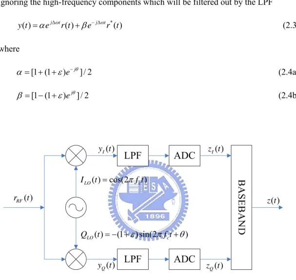
A generalized block-diagram of an analog I/Q based quadrature receiver [6], [7] is presented in Figure 2-1. The I/Q imbalance can be characterized by the amplitude

and phase imbalances. Let be the baseband representation of the

RF received signal ( )r t , we have that

( ) I( ) cos(2 c ) Q( )sin(2 c )

r t =r t π f t +r t π f t (2.1)

After passing the mixer and considering the effects of IQ imbalance and CFO, the received signals on the I branch and Q branch become

( ) ( ) cos( ) ( )(1 )sin( )

I I Q

y t =r t ∆ωt −r t +ε ∆ +ω θt (2.2a)

( ) _i( ) _q( )

(16)

14

( ) ( )(1 )sin( ) ( ) cos( )

Q I Q

y t = −r t +ε ∆ +ω θt +r t ∆ωt (2.2b)

where ∆ωt represents the effect of CFO. By defining and

ignoring the high-frequency components which will be filtered out by the LPF

* ( ) j t ( ) j t ( ) y t =αe ∆ωr t +βe− ∆ωr t (2.3) where [1 (1 ) j ]/ 2 e θ α _{= + +}ε − _(2.4a) [1 (1 ) j ]/ 2 eθ β = − +ε (2.4b)

LPF

ADC

( ) RF r t ( ) cos(2 ) LO c I t = π f t ( ) (1 )sin(2 ) LO c Q t = − +ε π f t+θ ( ) I y t ( ) Q y t ( ) I z t ( ) Q z t ( ) z t

Figure 2-1 Generalized I/Q Imbalance Model

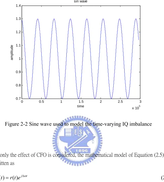
Considering the characteristic of the analog circuits, the phase error θ and gain error g (=1+ε) may change with time. Here a sine wave will be used to model the change of g and θ , as shown in figure 2-2.And equation (2.3) can be rewritten as

*

( ) ( ) j t ( ) ( ) j t ( )

y t =α t e ∆ωr t +β t e− ∆ωr t (2.5)

( ) _I( ) _Q( )

(17)

15 0 0.5 1 1.5 2 2.5 3 x 105 0.7 0.8 0.9 1 1.1 1.2 1.3 1.4 time am pl it u de sin wave

Figure 2-2 Sine wave used to model the time-varying IQ imbalance

If only the effect of CFO is considered, the mathematical model of Equation (2.5) can be rewritten as

( ) ( ) j t

y t =r t e ∆ω (2.6)

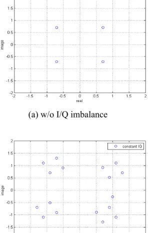
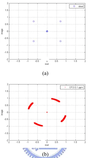
The effects of I/Q imbalance on the QPSK constellation is depicted in Figure 2-3. With the influences of I/Q imbalance, one constellation point will become four points because the interference of the image signal. By considering the effects of time-varying I/Q imbalance, the constellation will further shift a distance with time. Figure 2-4 shows the effects of CFO on QPSK constellation. It is obviously that the constellation points have rotated from the ideal positions eventually. If the rotation angle exceeds the decision boundary, it will cause the decision error.

(18)

16

(a) w/o I/Q imbalance

(b) with I/Q imbalanceIQ 1dB 20° and 2dB 10°

(c) with I/Q imbalance, time-varying 30%, IQ 1dB 20° and 2dB 10°

Figure 2-3 QPSK constellation, w/o Multi-path, w/o AWGN, (a) w/o I/Q imbalance (b) with I/Q imbalance (c) with time-varying I/Q imbalance

(19)

17

(a)

(b)

Figure 2-4 QPSK constellation (a) w/o CFO (b) CFO 0.1 ppm

2.2 Simulation Platform

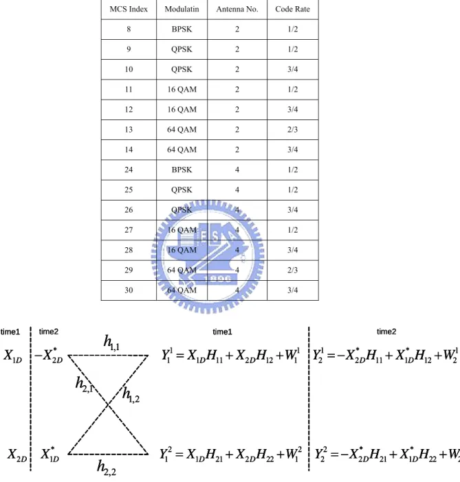
The simulation platform is MIMO-OFDM system. It is constructed according to the standard of IEEE. 802.11n. There are three main blocks, transmitter, channel model, and receiver. For the MIMO-OFDM system [9] operation in 20 MHz, it supports fourteen MCS (Modulation-Coding Scheme) sets, as shown in Table2-1, and can transmit data by 2x2 or 4x4 antennas. Each OFDM symbol is constructed from 56 tones, of which 52 are data tones and 4 are pilot tones. The tone mapping is identical to that in IEEE 802.11a[8] (subclause 17.3.5.9 in reference) except the 2 extra tones on either side.

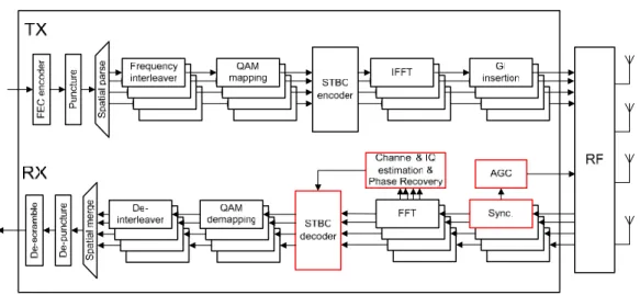
In the transmitter, the data will be encoded by Alamouti STBC (Space Time Block Code), as shown in Figure 2-5. Then the data will go through OFDM

(20)

18

modulation, and transfer from frequency domain signal to time domain signal by IFFT. In receiver, first step, it uses FFT to transfer received signal to frequency domain data; second, Equalizer will compensate channel effect then combine two stream data into original by Alamouti Decoder. The MIMO basic architecture is shown as Figure 2-6.

Table 2-1 MCS set

=

X H

+

X H

+

W

Y

= −

X H

+

X H

+

W

time1 time2 2 2 2 * * 2 1 1D 21 2D 22 1 2 2D 21 1D 22 2

Y

=

X H

+

X H

+

W

Y

= −

X H

+

X H

+

Y

=

X H

+

X H

+

W

Y

= −

X H

+

X H

+

W

time1 time2 2 2 2 * * 2 1 1D 21 2D 22 1 2 2D 21 1D 22 2

Y

=

X H

+

X H

+

W

Y

= −

X H

+

X H

+

W

1 1 1 * * 1 1 1D 11 2D 12 1 2 2D 11 1D 12 2

Y

=

X H

+

X H

+

W

Y

= −

X H

+

X H

+

W

time1 time2 2 2 2 * * 2 1 1D 21 2D 22 1 2 2D 21 1D 22 2

Y

=

X H

+

X H

+

W

Y

= −

X H

+

X H

+

W

(21)

19

Figure 2-6 MIMO Basic Architecture

AWGN, time-variant Doppler multipath, carrier frequency offset, phase noise, sampling clock offset and path loss are simulated in the channel, where the AWGN is added, the time-variant Doppler multipath is convoluted, CFO which joint phase noise is multiplied and SCO is convoluted with sinc wave to the Tx signal. The parameter of the AWGN channel is the signal-to-noise ratio (SNR) in dB, and for CFO and SCO is the frequency offset in ppm proportional to the carrier frequency and the symbol sampling frequency respectively. As for the multipath fading channel, the parameters include the channel type, the root-mean-square (rms) delay spread value and the tap numbers. The loop bandwidth and the loop time constant of the low-pass filter in phase-locked loop (PLL) decide the range of phase noise. 錯誤! 找不到參照來源。3 shows the practical and the baseband equivalent channel model.

RX RF

TX RF

DAC BPF PA Path Loss Interference Multipath AWGN BPF LNA VGA Time Variant (Doppler) TX IQ mismatch phase noise ADC CFO Noise Nonlinear RX IQ mismatch phase noise SCO Filter Imbalance Nonlinear Distortion Harmonic Harmonic

RX RF

TX RF

DAC BPF PA Path Loss Interference Multipath AWGN BPF LNA VGA Time Variant (Doppler) TX IQ mismatch phase noise ADC CFO Noise Nonlinear RX IQ mismatch phase noise SCO Filter Imbalance Nonlinear Distortion Harmonic Harmonic

(22)

(23)

Chapter 3 THE PROPOSED ALGORITHM

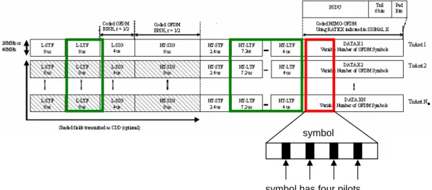
In the standard of 802.11n, each MIMO OFDM symbol has four pilots. These pilots can be used to estimate the Time-variant IQ Imbalance and track the residue CFO in the received symbol. In section 3.1, an adaptive IQ Imbalance estimation scheme will be introduced. And in section 3.2, another algorithm for phase recovery will be described.

3.1 Adaptive Estimation for Time-varying I/Q

Imbalance

Figure 3-1 lists the data sheets of the packet format used for adaptive I/Q estimation. L-LTF and HT-LTF are used for the adaptive coefficients initialization and pilots are used for adaptive I/Q estimation. In equation (2.5), the problem of time-varying I/Q imbalance is described by the received data and two parameters, α and β. Since the received data is known, the main effort on solving the I/Q imbalance becomes “how to find the value of α and β”. In this thesis, the condition of time-varying I/Q imbalance is considered. Because the values of α and β will change with time, the one-shot approaches can not detect the variation of α and β between symbols and is not suitable for the estimation. The following equation is used for the compensation of I/Q imbalance when α and β are acquired.

2 2 * ( ) *( ) ( ) Z f Z f R f α β α β − − = − (3.1)

(24)

22

where Z is the actual received symbol and R is the compensated received symbol. Equation (3.1) can be further expressed as the follow 2-by-2 matrix form:

2 2 2 2 ( ) ( ) *( ) Z f R f Z f α β α β α β ⎡ ₋ _{⎤ ⎡} _⎤ = ⎢ _{⎥ ⎢} _⎥ − − − ⎢ ⎥ ⎣ ⎦ ⎣ ⎦ (3.2) Let W f( ) ₂α ₂ α β = − 、 W( f) 2 2 β α β − − =

− represent the adaptive coefficients, Equation(3.2) can be simplified as

[

]

( ) ( ) ( ) ( ) *( ) Z f R f W f W f Z f ⎡ ⎤ = − _⎢ _⎥ − ⎣ ⎦ (3.3) The adaptive estimation of r in equation (2.5) can be attain by updating the adaptive coefficients W according to the following LMS rules

1_{( )} _{( )} _{( )}* _{( )} i i i i W + f =W f +µZ f e f (3.4a) 1₍ ₎ ₍ ₎ ₍ ₎* ₍ ₎ i i i i W + −f =W −f +µZ −f e −f (3.4b) * ( ) ( ) ( ( ) ( ) ( ) ( )) i i i e f =Y f − W f Z f +W −f Z −f (3.5a) ( ) i( ) Y f R f = − (3.5b) where i( )

e f is the ith error function, µ is the step-size parameter. Moreover, Y is

the ideal received value at the pilot tone. In the MIMO-OFDM system, one receiver will receive data from different transmitters at the same time. Assume the channel frequency response H is acquired, the ideal received data of the ith antenna can be express as the follow equation:

4 1 ( ) ( ) ( ) i ij j j Y f H f P f = =

∑

(3.6) where P is the ideal value of pilot in the MIMO-OFDM symbol and Hij is the channel

frequency response between the transmit antenna j and the received antenna i.

For the parameters which are real numbers, table 3-1 illustrates how equation (3.4) works. Take the first row of table 3-1, the value of e(f) is positive. That means the actual received data R(f) is small than the ideal received data Y(f). Since the values of Z(f) and Z(-f) are both positive, according to equation (3.4), the value of both W will increase. Finally, the i+1th R(f) will increase to minimize the error e. So

(25)

23 W can converge to the right value and the received data can be corrected. For the

complex numbers, the same results can also be carried out, but conjugation is needed for Z because the multiplication of the image part will become negative.

Figure 3-1 Data sheets of MIMO-OFDM packet format used for adaptive I/Q estimation

Table 3-1 Real number scenarios of equation (3.4)

I i+1 Z(f) Z(-f) e(f) W(f) W(-f) R(f) + + + ↑ ↑ ↑ + - + ↑ ↓ ↑ + + - ↓ ↓ ↓ + - - ↓ ↑ ↓

An important factor affecting the adaptive estimation is the convergence rate. Although the LMS is the simplest adaptive implementation in terms of complexity, it suffers from a slow convergence rate. While considering the effects of time-varying I/Q imbalance, the variation of W must be detect between the data symbols. Thus, the only information can be used in the data symbol is the pilots. This problem becomes worse because there are only four pilots in each MIMO-OFDM symbol. In LMS, the coefficients in equation (3.4a) and (3.4b) are usually initiated with zeros as their initial value. In order to improve the convergence rate, a preamble based method [2] is used to calculate the better initial values by preambles. Step-size is another parameter which will affect the convergence rate, because it directly affects how quickly the coefficients will converge. If it is very small, then the coefficients change only a small

symbol has four pilots symbol

(26)

24

amount at each update, and the coefficients converges slowly. With a larger step-size, the coefficients may converge more quickly. However, when the step-size is too large, the coefficients may change too quickly and the adaptive estimation will diverge. Under the condition of I/Q imbalance with time-varying 30%, the step-size is set to 1% in order to get better performance.

Figure 3-2 show the flow-chart of adaptive I/Q estimation. After the FFT transforms the received data from time domain to frequency domain, if the output of FFT is the data symbol, the pilots in the symbol will be extracted to do the I/Q parameter estimation. Once the adaptive coefficients are acquired in the step of I/Q parameter estimation, they will be used to compensate the received data and the compensated data will be send into the STBC decoder.

FFT output I/Q Parameter Estimation Extract Pilot I/Q Compensation Input symbol into STBC decoder Output data symbol? Yes No

Figure 3-2 Flow-chart of adaptive I/Q estimation

(27)

25

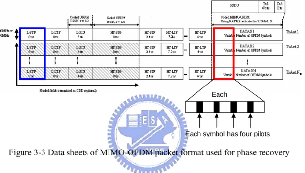
Because the estimation and compensation of CFO is not perfect [3], the received data will be affected by the residue CFO. The remaining CFO will bring on the problem of phase rotation which can’t be neglected even if the CFO is very slight, and the phase deviation of OFDM symbols will also grow with the increasing of the symbol indexes. If the phase rotation is not corrected, finally, the rotation angle will exceed the limitation of modulation decision boundary and cause the decision error. Fortunately, the pilot can be used to detect the remaining CFO in each symbol. Figure 3-3 lists the data sheets of the packet format used for phase recovery. L-STF is used for the CFO estimation and pilots are used for phase recovery.

Figure 3-3 Data sheets of MIMO-OFDM packet format used for phase recovery The ideal received data of the ith antenna at the pilot tone can be acquired according to equation (3.6). The actual received data, R, at the pilot tone will be the ideal received data multiply j

eθ, where θ is the phase rotation angle.

4 1 ( ) ( ) ( ) j i ij j j R f H f P f eθ = =

∑

(3.7)

The phase difference j

eθ between the ideal received pilot P and the actual

received pilot R can be acquired by dividing R with Y.

4 1 4 1 ( ) ( ) ( ) ( ) _{( )} _{( )} j ij lj j j i i ij lj j H f X f e R f e Y f H f X f θ θ = = =

∑

=

∑

(3.8)

Thus, the phase rotation can be corrected by multiply the received data with j e−θ

according to the following equation

Each symbol has four pilots Each

(28)

26

( ) ( ) j f

i i

Y f =Z f e− ∆ (3.9)

Figure 3-4 show the flow-chart of phase recovery. After the FFT transforms the received data from time domain to frequency domain, if the output of FFT is the data symbol, it will be compensated by the accumulated phase error first. The accumulated phase error is the phase error accumulated before the phase error estimation at this time. Then the pilots in the symbol will be extracted to do Phase error estimation. Once phase error is acquired in the step of phase error estimation, it will be used to compensate the received data and be accumulated. Finally, the compensated data will be send into the STBC decoder

FFT output Phase Error Estimation Extract Pilot Phase Error Compensation Input symbol into STBC decoder Output data symbol? Yes No Compensate Accumulated Phase Error Accumulate Phase Error

(29)

Chapter 4 SIMULATION RESULTS

To evaluate the proposed algorithm, a typical MIMO-OFDM system based on IEEE 802.11 wireless LANs, TGn sync proposal technical specification is used as a reference-design platform. In section 4.1, the simulation result of Adaptive Estimation for Time-variant IQ Imbalance will be mentioned. And in section 4.2, the performance of phase recovery will be presented.

The simulation environment below is based on the following conditions: z MIMO-OFDM system in 20 MHz

z PACK no. is 1000 z PSDU is 1024 bytes z MCS is 13

z Decoder using soft Viterbi decoder

z Multipath Model : TGnE (rms delay spread 100 and tap numbers 15)

4.1 Adaptive I/Q Estimation for Time-variant IQ

Imbalance

(30)

28

The simulation results of the adaptive I/Q estimation are shown in Figure 4-1. Table 4-1 is the performance summary of the adaptive I/Q estimation. From the simulation results, the performance loss of the adaptive I/Q estimation is about 4 dB under the constant I/Q imbalance and is about 7 dB under the I/Q imbalance with time-varying 30%. Compared with the constant compensation, the adaptive I/Q estimation can improve the performance about 5 dB under the I/Q imbalance with time-varying 30%.

14 16 18 20 22 24 26 28 30 32 34 0 0.1 0.2 0.3 0.4 0.5 0.6 0.7 0.8 0.9 1 PER vs SNR SNR PER

2x2 Constant IQ Constant Comp. 2x2 Constant IQ Adaptive Comp. 2x2 Time-varying IQ 0.3 Constant Comp. 2x2 Time-varying IQ 0.3 Adaptive Comp. Ideal Comp.

wo Comp.

Figure 4-1 PER vs SNR, MCS 13,TGnE, IQ 1dB 20° and 2dB 10°, 2x2 MIMO-OFDM system

Table 4-1 Performance summary of the adaptive I/Q estimation

condition Required SNR @ PER = 0.1%

Constant I/Q , w/o adaptive 20.2

Constant I/Q , with adaptive 22

Time-varying, w/o adaptive 30

Time-varying, with adaptive 25

(31)

29

4.2 Phase Recovery

Figure 4-2(a) and 4-3(a) show how worse the 64 QAM constellations will be without phase recovery on the 2x2 and 4x4 MIMO-OFDM system. It is obviously that the constellation points have rotated over the decision boundaries, thus correct demodulation is no longer possible. Figure 4-2(b) and 4-3(b) show that phase recovery does correct the CFO estimation errors and make the 64 QAM constellations better.

Figure 4-2 Constellation of CFO 50 ppm under 2x2 MIMO-OFDM system (a) w/o phase recovery (b) with phase recovery

Figure 4-3 Constellation of CFO 50 ppm under 4x4 MIMO-OFDM system (a) w/o phase recovery (b) with phase recovery

-2 -1.5 -1 -0.5 0 0.5 1 1.5 2 -2 -1.5 -1 -0.5 0 0.5 1 1.5 2 -2 -1.5 -1 -0.5 0 0.5 1 1.5 2 -2 -1.5 -1 -0.5 0 0.5 1 1.5 2 -2 -1.5 -1 -0.5 0 0.5 1 1.5 2 -2 -1.5 -1 -0.5 0 0.5 1 1.5 2 -2 -1.5 -1 -0.5 0 0.5 1 1.5 2 -2 -1.5 -1 -0.5 0 0.5 1 1.5 2 (a) (b) (a) (b)

(32)

30

Figure 4-4 shows the PER versus SNR with CFO 50 ppm on the 2x2 MIMO-OFDM system. The square line represents the case without phase recovery. The PER approaches one without phase recovery even when the SNR is 25 dB. The triangular line represents the case with phase recovery. The PER can reach under 0.1 when the SNR is about 19.9 dB. The circle line represents the case with ideal compensation. The PER can reach under 0.1 when the SNR is about 17.9 dB. The performance loss of phase recovery on the 2x2 MIMO-OFDM system is about 2dB.

Figure 4-4 PER vs SNR, CFO=50 ppm, 2x2 MIMO-OFDM system

14 16 18 20 22 24 26 0 0.1 0.2 0.3 0.4 0.5 0.6 0.7 0.8 0.9 1 PER vs SNR SNR PER 2x2 50ppm wo Comp. 2x2 50ppm phase recovery 2x2 50ppm Perfect Comp.

(33)

31

Figure 4-5 shows the PER versus SNR with CFO 50 ppm on the 4x4 MIMO-OFDM system. The square line represents the case without phase recovery. The PER approaches one without phase recovery even when the SNR is 25 dB. The triangular line represents the case with phase recovery. The PER can reach under 0.1 when the SNR is about 19.4 dB. The circle line represents the case with ideal compensation. The PER can reach under 0.1 when the SNR is about 18.7 dB. The performance loss of phase recovery on the 4x4 MIMO-OFDM system is about 0.7 dB.

Figure 4-5 PER vs SNR, CFO=50 ppm, 4x4 MIMO-OFDM system

15 16 17 18 19 20 21 22 23 24 25 0 0.1 0.2 0.3 0.4 0.5 0.6 0.7 0.8 0.9 1 PER vs SNR SNR PER 4x4 50ppm wo Comp. 4x4 50ppm phase recovery 4x4 50ppm Perfect

(34)

32

Chapter 5 HARDWARE IMPLEMENTATION

OF PHASE RECOVERY

Due to the variables in Verilog only have finite precision, the word length of variables in the Matlab platform must be decided by the procedure of Fixed-point. Figure 5-1 shows the flowchart of Matlab to Verilog design. Fixed-point simulations are performed to decide the word length of variables in the Matlab platform and ensure that these changes will not degrade system performance seriously. This is a trade-off between the cost and the performance. Once the fixed-point simulations are done, the input and output data generated by the Matlab platform will be fed into the Verilog module to verified the correctness of the desired functionality in Verilog. If the output data of Matlab is completely the same as the one of Verilog, the transformation from Matlab to Verilog is done. The data flow of phase recovery is shown in figure 5-2. The whole algorithm of phase recovery can be divided into tow main function blocks, Phase Error Estimation, and Phase Error Compensation. After passing the FFT, the received data will be transformed from time domain to frequency domain. The phase error estimation will take both the outputs of FFT and channel estimation as the inputs. After the phase error is acquired, the phase error compensation will use it to compensate the received data and pass the compensated data to the STBC decoder.

(35)

33

(36)

34

Figure 5-2 data flow chart of phase recovery

Figure 5-3 shows the input/output port definition of phase error estimation. Phase error estimation will take the received pilots and channel frequency responses as the inputs and its outputs will be the estimated phase error. Figure 5-4 is the hardware architecture of phase error estimation. In this block, the four ideal pilots of each antenna will multiply with their own channel frequency responses and be summed up to acquire the ideal received data at the pilot tone. After the ideal received data is carried out, the actual received data will be divided by the ideal received data to acquire the estimated phase error. The gate count of phase error estimation is about 40K in TSMC 0.13µm CMOS process. Pilot_I Pilot_Q CLK RESET H11_I H11_Q H12_I H12_Q H13_I H13_Q H14_I H14_Q CFO_I CFO_Q

(37)

35

Figure 5-4 Hardware Architecture of Phase Error Estimation

Figure 5-5 shows the input/output port definition of phase error compensation. Phase error compensation will take the received pilots and the estimated phase error as the inputs and its outputs will be the compensated data. Figure 5-6 is the hardware architecture of phase error compensation. In this block, it will first sum up the four phase errors estimated by the phase error estimation. Then the summation of the phase errors will be divided by 4 to get the average. The function of abs is to get the amplitude of the average phase error. It will get the summation of the squares of the image part and real part of the average phase error, and then calculate the square root of the summation. The average phase error will be divided by the square root to get the normalized phase error. Once the normalized phase error is carried out, the ACC will sum up the normalized phase error with the previous one and the received data will be compensated by multiplying the conjugate of the normalized phase error. The gate count of phase error compensation is about 200K in TSMC 0.13µm CMOS process.

(38)

36 PH ASE ER RO R COMPENSAT ION CFO_I*4 CFO_Q*4 DATA_I*56 DATA_Q*56 CLK RESET Comp_DATA_I*56 Comp_DATA_Q*56 Enable Out_Valid

Figure 5-5 Input/output port definition of Phase Error Compensation

(39)

37

Chapter 6 CONCLUSION

Carrier Synchronization plays an important role in MIMO-OFDM systems. The presence of I/Q imbalance in an RF front-end introduces an image interference and the CFO estimation errors degrades the system performance. In this thesis, a pilot-based scheme for the time-varying I/Q imbalance and phase recovery has been proposed. The improvement of adaptive I/Q estimation is about 5 dB under the time-varying I/Q imbalance with variation 30% and the phase recovery can correct the CFO estimation errors effectively. Table 6-1 shows the comparison result of I/Q imbalance with other methods. From this table, the proposed algorithms have lower computational complexity and can satisfy the required system performance. Finally, the phase recovery is implemented by TSMC 0.13 µm CMOS process and the gate count is about 240 K.

(40)

38

Table 6-1Comparison with other methods

Ref [11] Ref [14] Ref [15] This Work System SISO 2x2 MIMO 2x1 MIMO 2x2 MIMO Method FIR Filter &

LS RLS & MMSE LS

Adaptive & LMS Computational Complexity High High High Low

Packet Format User Defined User Defined IEEE 802.11n IEEE 802.11n

Time-varying Imbalance No No No No Channel No No No Yes IQ Parameter (Maximum Value) g = 1 dB Ө = 5 ° g = 0.45 dB Ө = 2.81 ° g = 2 dB Ө = 5 ° g = 2dB Ө = 20 ° Constant Imbalance 1 dB SNR loss 2.5 dB SNR loss 0.5 dB SNR loss 2.2dB SNR loss Performance Time-varying

Imbalance N/A N/A N/A

5dB SNR improvement

(41)

Bibliography

[1] TGn Sync Group, IEEE P802.11 Wireless LAN - TGn Sync Proposal Technical Specification, Proposal of IEEE802.11n, IEEE Document 802.11-04/889r4,

[2] Wei-Chi Lai and Terng-Yin Hsu, The Study of All-Digital compensation for I/Q

Mismatch with Frequency Dependent Imbalance in MMO-OFDM Baseband Designs, 2006.

[3] Jui-Yuan Yu, Ming-Fu Sun, Terng-Yin Hsu, and Chen-Yi Lee, A Novel Technique

for I/Q Imbalance and CFO Compensation in OFDM Systems, 23-26 May 2005

Page(s):603-6033 Vol.6 Digital Object Identifier 10.1109/ISCAS.2005.1466014 [4] Hung-Kuo Wei and Chen-Yi Lee, A Frequency Estimation and Compensation

Method for High Sped OFDM-based WLAN System, 2002

[5] Alireza Tarighat, Rahim Bagheri, and Ali H. Sayed, Compensation Schemes and

Performance Analysis of IQ Imbalances in OFDM Recievers, IEEE

TRANSACTION ON SIGNAL PROCESSING, VOL 53, NO. 8, AUGUST 2005 [6] M. Valkama , M. Renfors, and V. Koivunen, “Compensation of

frequency-selective IQ imbalances in wideband receivers models and algorithms”,

Wireless Communications, 2001. (SPAWC '01). 2001 IEEE Third Workshop on Signal Processing Advances in 20-23 March 2001 Page(s):42 – 45

[7] Francois Horlin, Stefaan De Rore, Eduardo Lpoez-Estraviz, Impack of Frequency Offset and IQ Imbalance on MC-CDMA Reception Based on Channel tracking, IEEE JOURNAL ON SELECTED AREAS IN COMMUNICATONS, VOL. 24, NO. 6, JUNE 2006.

[8] Wireless LAN Medium Access Control (MAC) and Physical Layer (PHY)

(42)

40

[9] M. Valkama , M. Renfors, and V. Koivunen,,.”Blind source separation based I/Q imbalance compensation,” in Proc. IEEE Symposium 2000 on Adaptive Systems for Signal Processing, Communications and Control, Lake Louise, Alberta, Canada, Oct. 2000, pp 310-314.

[10] K.P. Pun, J.E. Franca, C. Azeredo-Leme, C.F. Chan,C.S. Choy, “Correction of frequency-dependent I/Q mismatches in quadrature receivers,” IEEE Electronics Letters, Volume 37, Issue 23, Page(s):1415–1417, Nov 2001.

[11] X. Guanbin, S. Manyuan, L. Hui, “Frequency offset and I/Q imbalance compensation for direct-conversion receivers,” IEEE Transactions Wireless Communications, Volume 4, Issue 2, Page(s):673–680, March 2005.

[12] T.M. Ylamurto, “Frequency domain IQ imbalance correction scheme for orthogonal frequency division multiplexing (OFDM) systems,” IEEE Wireless Communications and Networking, Volume 1, Page(s):20–25, March 2003.

[13] R.M. Rao, B. Daneshrad, “I/Q mismatch cancellation for MIMO-OFDM systems,” 15th IEEE International Symposium Personal, Indoor and Mobile Radio Communications (PIMRC), Volume 4, Page(s):2710-2714, Sept. 2004.

[14] R.M. Rao, B. Daneshrad, “Analog impairments in MIMO-OFDM systems,”IEEE Transactions on Wireless Communications VOL. 5, NO. 12, December 2006. [15] Alireza Tarighat, Ali H. Sayed, “MIMO OFDM Receivers for Systems with IQ

Imbalances, ”IEEE Transactions on Signal Processing, VOL. 53, NO. 9, September 2006

應用於無線多輸入多輸出基頻處理器載波同步之研究

國

立

交

通

大

學

網路工程研究所

碩

士

論

文

應用於無線多輸入多輸出基頻處理器載波

同步之研究

The Study of Carrier Synchronization for MIMO-OFDM

Baseband Designs

研 究 生：陳信男

指導教授：許騰尹 教授

應用於無線多輸入多輸出基頻處理器載波同步之研究

The Study of Carrier Synchronization for MIMO-OFDM Baseband

Designs

研 究 生：陳信男 Student：Hsin-Nan Chen

指導教授：許騰尹 Advisor：Terng-Yin Hsu

國 立 交 通 大 學

網 路 工 程 研 究 所

碩 士 論 文

摘要

Abstract

Acknowledgement

Contents

List of Figures

List of Tables

Chapter 1

INTRODUCTION

Chapter 2

SYSTEM MODELING

2.1 Modeling and Effects of Carrier Synchronization

LPF

LPF

ADC

ADC

2.2 Simulation Platform

h

h

h

h

X

−

X

X

X

Y

=

X H

+

X H

+

W

Y

= −

X H

+

X H

+

W

Y

=

X H

+

X H

+

W

Y

= −

X H

+

X H

+

W

h

研究生：陳信男

指導教授：許騰尹教授

研究生：陳信男 Student：Hsin-Nan Chen

國立交通大學

網路工程研究所

碩士論文