On-line adaptive tuning for PID controllers

(1)

PID

CONTROL

On-line adaptive tuning for

PID

controllers

H.-P.Huang, M.-L.Roan and J.-C.Jeng

Abstract: Adaptive and robust designs are two major approaches to deal with possible modelling errors in a control system. This paper proposes an adaptive control system for on-line tuning of PID controllers for SISO systems. The proposed system comprises of two adaptive loops. The first loop monitors and tunes the controllers on-line to ensure the system is robustly stable. This first loop enables the system to achieve robust stability over a wide range of possible modelling errors without trading off performance against nominal design. When modelling errors occur, the second adaptive loop conducts recursive on-line identification and retunes the controller. Because the nominal model is corrected on-line, directly following the on-line identification the system can continue as a new nominal system which is designed to have tight control performance. Numerical examples are presented to illustrate this adaptive control with two loops.

List of symbols

transfer function of the IMC controller transfer function of the plant

transfer function of the conventional controller gain

transfer function of the multiplicative modelling error

parameter vector

Laplace transform variable time .

output

model output by the same input

Greek symbols a: 6: Sampling interval A: difference

A:

eigen value w : frequency

4:

parameter sensitivity vector @: parameter sensitivity matrix

z: time constant c: singular value

Superscripts

constant in the realisable PID controller

nominal estimated value T: transpose Subscripts 0: initial D : derivative R: reset

f :

filter i: integral p : plant 0 IEE, 2002

IEE Proceedings online no. 20020099

DOI: 10.1049/ip-cta:20020099 Paper first received 12th November 2001

The authors are with the Department of Chemical Engineering, National Taiwan University, Taipei, Taiwan 10617

60

1 Introduction

Dynamics of industrial plants are usually not completely known and are subject to change from time to time. In dealing with the control of such plants, robust control design and adaptive control design are two major approaches being used [l]. Each approach has its merits and inevitable disadvantages. For example, in robust control design, the system can remain stable subject to a set of modelling errors. However, owing to these modelling errors, the nominal performance of the system is traded off to secure robust stability. As the set of possible modelling errors expands, the performance of the nominal system becomes more conservative. Overviews of robust designs of such controllers can be found in [2] and [3]. On the other hand, theories and applications of adaptive control, especially self-tuning control, have been extensively reported in survey papers and books [4-61. In adaptive design, good system performance is maintained by conducting self-tuning when the system deviates from nominal. Nevertheless, in general, there is a fundamental conflict between implementing self-tuning and the regular objectives of control [7], because special inputs are required to achieve repeated signals for on-line identification as an important ingredient of the self-tuning system. The stability of these self-tuning systems is another important issue. Although this issue has been addressed by researchers [ 6 ] and despite a great deal of progress in dealing with bounded disturbances [8-111, the stability of these systems is still a challenge in practical systems [lo, 121. For the reasons mentioned, adaptive systems are usually so sophisticated that they have to be maintained by well-trained personnel.

To the merits of both approaches, a system with dual adaptive loops (DAL) to enhance a conventional single- loop PID control system is presented. The conventional PID controller is designed to be stable over a small range of uncertainties to ensure tight nominal Performance. The robustness of performance and stability is ensured by the dual adaptive loops.

The first adaptive loop conducts on-line tuning of the PID controller by adjusting an IMC filter to ensure stability robustness before updating to a new nominal model. Since

(2)

adaptation is done without estimating changes to the nominal model, it is performed in a direct manner. The second adaptive loop identifies the changes to the nominal model and tunes the controller accordingly. Because on-line identification is used, correction of the nominal model is performed in an indirect manner, i.e. by updating the nominal model of the process first and then changing the controller. During on-line identification, dead time and other parameters in the process are estimated at the same time. As the estimation of dead time needs nonlinear least squares computations, a Newton-like algorithm is also presented. The dual-loop adaptive system is then applied to a single-loop system where the nominal model is first order with dead time.

2 PID controller design for nominal system

Since the 1980s, the IMC principle has been a useful tool for designing feedback controllers. The design methodol- ogy focuses mainly on the use of an 1MC filter and the inverse of a nominal model for the open-loop process, i.e. .G,(s). In this way, the feedback controller of a closed-loop

system can be synthesised as

where C(s) is obtained by

Here,

Gp

represents a nominal model of GI,, represents the invertible part of

ep,

and F(s) is an IMC filter.

As a linear system with general dynamics, Gp is consid- ered to be represented by a model in terms of the following transfer function:

(3) where N(s) and D(s) are rational polynomials of s. For most processes with high-order dynamics, their dynamics are usually modelled as the first-order dynamics plus dead time, that is,

kPe-Os

G,(s) =

-

zs

+

1 (4)

In other words, all the higher order lags in (3) are lumped together to form an effective dead time.

To synthesise a controller' via IMC for Gp in (4), a nominal model and filter are chosen as follows:

1

F(s) = - ZfS+ 1

The corresponding IMC-PID controller is

(5) where z

+

0.50 k, = ~ 2f

+

0 ZR = z

+

0.50 zg = - 22

+

e

7 (7)

o.sZfe

zf

+

e

a=-

Because

c,

in (5) is used, model mismatch is inevitable even though the model for Gp in (4) is perfect. This model mismatch is given as follows:

G t ( s ) =

2

- 1 GP kp N(s)(?s

+

1) 1

+

0.58s - _e - 1 (8) kp D(s) 1 - 0.58s - - _

In the presence of this model mismatch, the time constant of the IMC filter, zf, has important effects on the performance and robustness of the closed-loop system. Rivera et al. [ 131 discussed this issue in detail with regard to this IMC-PID controller. They show that the controller gives an optimal value for the ISE performance measure at T f / Q 0.65. The setting for ?,in a non-adaptive system has to ensure robust stability over all possible modelling errors and, thus, must not use small values of zf/0 ratio. As a result, the nominal performance has to be traded off against stability.

With this DAL scheme, the system allows zf to have lower values which, in turn, gives tighter nominal performance. If modelling errors exist or changes to the model occur, the first loop of this DAL adaptive system starts to detune the controller on-line to ensure robust stability. As

detuning the controller degrades the performance of the system, the second adaptive loop begins estimating the changes to the system to retune the controller. Thus the system will resume as a new nominal system that is designed to give tighter performance.

3 Direct adaptation of 7 , for stability robustness

In this Section, direct adaptation to achieve robust stability by adjusting an IMC filter is discussed. In the IMC design, the time constant of the filter, zf, has to be chosen properly to provide stability robustness subject to modelling mismatch. However, any choice of constant value for zf has to deal with a trade-off between performance and stability robustness. Thus, it is desirable to start with a smaller value of zf which gives satisfactory nominal responses and then to change the value of

zf

on-line to ensure robustness when model mismatches jeopardise the stability of the system.

To develop the adaptive law for this purpose, first, a nominal value for zf should be assigned. Besides the minimum ISE measure, the overshoot produced by the system is also an important factor to be considered. Fig. 1 shows the resonance peak gain and overshoot of this IMC- PID control system. According to Fig. 1, a value of 0.5 for T f / Q will produce no more than 5% overshoot in the nominal case.

61

(3)

1 .80

-

1.60 -

$

1.40- C C

P

??

<

1.20

-

Q 1.00 - - - - - - 80 70 60

g

-50 5- 0 .c L -40 a, (51 -30 0 Q ?I 20 10 TF Fig. 1

PID control system

T ~ = T ~ / O where 8 is dead time in the first-order model plus dead time

Peak resonance (M,,) andpercentage overshoot (PO) f o r an IMC-

With this setting for zf, the nominal system will have a gain margin equal to 3. Note that the gain margin of the system is given by

GM=Z?(;+l) (9)

Next, we look at how zfshould be changed to keep the system robust. The following two properties will be useful for deriving the adaptive law for

zf

and their proofs are given in the Appendix (Section 9).

Property 1: For Gp(s) in (4) and an IMC controller design based on (5), the initial slope of the system output, after the effective dead time, is given by

Notice that the result is derived based on a model of (4). For a higher order system, the resulting effective dead time in terms of 0 in this model will be larger than the true one. As a result, the output, y, at t=O+ will have non-zero slope. Thus, with this slope, (4) can apply to this case only approximately.

Property 2: For Gp(s) in (3), which is open-loop stable and is strictly proper, there exists zf such that Vzfz z f , and the IMC controller can stabilise the closed-loop system.

According to property 1, a nominal system will yield an initial slope equal to 1 /zf in response to a stop change. Any changes in kp or z will disturb the initial slope of y from its nominal value. Notice that the complementary sensitivity function of this IMC-PID control system is given by

--os

T = t:

( ~ f

+

0.56')s

+

e-'' 1

+

0.58s

When Q is small, the bandwidth of the system is approxi- mately given by [ 131

1

O b 2 -

0

+

zf

Since zf is assigned to be 0.5 times 0, we have

To keep the initial slope of the response unchanged regardless of the existence of model errors, the bandwidth of the system must remain constant. Accordingly, the performance of the closed-loop system will remain robust to the model mismatch.

It is, then, clear that zfmust be adjusted to compensate for the change in the initial slope in order to achieve robust performance. To develop an algorithm for this purpose, let us define the following:

zj

=the initial value of zr= 0.58',

7

; = a new target value to which zf is to be _adjusted,

z? =the nominal designed value of zf= 0.58.

Here, 8' is dead time in the nominal model,

e

is effective dead time found in the actual response. Then, the algorithm for adapting tf is obtained as follows:

provided that y can be measured or estimated.

In practice, the estimation of j , by taking numerical derivative will be sensitive to measuring noise. To estimate j , at t=O, starting from the time instant at the effective dead time, three or more values of y separated by a small sampling interval (i.e. 8 ) are taken. These data are then fitted to a straight line. The_ slope of this line is then taken as the estimate of y at t= 8. This part of the adaptation is made at the very first stage right after the system's effective dead time.

On the other hand, achieving stability of the system requires examining whether there is diverging or persis- tently oscillating errors in tracking the set-point. According to property 2, whenever modelling errors jeopardise the stability of the system, by increasing ?f to a larger value, the system can eventually be stabilised. In contrast to modelling errors which jeopardise the stability of a closed-loop system, in some cases, modelling errors may make the system move towards a more favourable response than its nominal one. If so, changing zf will not be

necessary in such cases. Thus, adaptation of zr is necessary only if the system fails to track the set-point well and only if significant modelling errors are detected. This part of the adaptation is made until the response approaches the set-point.

An adapting algorithm is thus given as follows:

Here, t, is the moment when the response first approaches its target value, e(t) = r

-

y(t), and j ( t

I

t -

S)

is the model output using all the data up to t - 6. In other words, y ( t ) - jj(t

I

t - 6) is a one-step ahead predictive error which is used to detect the existence of modelling errors. The adaptive law given in (15) has the following implications:

1. When the nominal model is perfect, the value of zf will remain unchanged. Thus, the desired nominal performance can be obtained.

2 . When modelling errors exist but tracking errors are

small, model mismatch will not seriously jeopardise the control performance. In such cases, the value of zf will only be detuned slightly.

3. The value of zfwill stop increasing if the PID control IEE PTOC -Control Theory Appl, Vol 149, No I , January 2002

(4)

can enable the system output to reach and stay at the constant set-point.

-To summarise this direct adaptive law used to achieve system robustness,

zf

is adjusted according to the following:

- aj(

16 ; P"))

aj(

16; pi')) @( 16; P'")

-

. . .

aP

1 aP2 aps

aj(2s; P'") aj(26; P(')) @(26; P"')

aP

1 aP2 aP,

@(NG; ~ ( ' 1 ) aF(N6; P@) aP(N6; P'")

-

aPl aP2 aPs

-

...

. . . . . . . . . ... ...

where

7 ) = 7; = 0.58 for t < to.l

7 ) = 0.56z~y(to,,) for t

>

to., (1 7)

Here, to. I and to.9 denote the times at which y(t) reachesjhe values of 10% and 90% of the set-point, respectively. 8 is an estimated value of the time delay obtained through regression analysis around the data in the neighbourhood OfY(t0 1).

4 Indirect adaptation for nominal performance

According to the direct adaptive adjustment of zf depicted above, the value of zfwill float. In cases where the change of the initial derivative of the responses cannot be clearly identified, the value of -7, will continue increasing as long

as modelling errors exist. To bring this Z~ back to its

nominal value, the nominal model has to be updated on-line. Updating the nominal model and the controller using on-line algorithms is the main goal of indirect adaptive control. To estimate changes of the process model using on-line algorithms is known as on-line identification. Usually, least squares methods, especially linear least squares, are used for this purpose. In general, adaptive control with on-line identification experiences bottlenecks. First, on-line identification conflicts with the control objec- tives. As the control system brings the system back to its target as quickly as possible, the identification process perturbs the system by means of external signals (such as a sequence of set-point changes or some specially designed driving signals) in order to generate persistent excitations. Second, on-line identification itself encounters technical bottlenecks. One of the difficulties is in the estimation of dead time. Quite a bit of research on adaptive control with respect to unknown dead time has been reported in the literature [ 14-17]. Disadvantages of these methods include the large number of parameters needed and the conver- gence of the algorithms. As a matter of fact, estimation of dead time together with other system parameters is a nonlinear optimisation problem, so that linear least squares algorithms are not directly applicable. As a result, recursive algorithms for on-line identification and adaptive control are difficult to apply. In this dual-loop adaptive system, the indirect adaptive control includes on-line estimation of a nominal model of (4) and on-line computation of the controller parameters in (6).

For on-line identification, a model output is computed according to

where P =

{kp,

Q,

e }

is the parameter set of the model. Then, P is determined by minimising as follows:

-I(?; P) = [v(t)

J:

-5(t;

P)]*dt (19)

IEE Proc.-Control Theory Appl., Yol. 149, No. 1. January 2002

To derive an on-line estimation algorithm for it is assumed that the model output, j is differentiable with respect to the parameter vector,

P.

In other words, it is assumed that there always exists a small positive number, E ,

such that o(E*) is negligible and the following holds: AP

25

j ( t ;

P)

+

t(b(t; P)T - IAPI

+

o ( 2 ) (20)

where 6 is a small perturbation to the parameter p I , and

j ( t , p I ) can be obtained by integrating the differential

equation as described by the model in (18) using u(t) as the deriving input.

Let

V , ( N ; P'") = [Y(N)

-

Y ( N ; P'")]'[Y(N)

-

Y ( N ; P('))]

(22) where the superscript i designates that the referredAvalue is taken at the ith iteration. For convenience, Y ( N ; P")) will

be abbreviated as Y,(N) and @(N, P'") as in the following. Then, we have AV,(N =

v,+1

(N> - V,W) = [ Y ( N ) - Y ( N ; p,+l)ITIY(N

-

Y ( N ; Pl+i)l - [Y(N) - Y ( N ; P,)]'[Y(N) - Y ( N ; PJ] (23) 63

(5)

If we let

AP(') =

{[@i(N)]T[@i(N)])-'

( [ @ i ( N ) ] T [ Y ( N )

-

Y i ( N ) J (25) and

where @, designates @(N, P(')). It is thus found that AV,(N) 5 0 , VO 5 p, I 2 (27) Because J.(@,(@~@,)-'@~) 2 0, it is evident that AV,(N) 5 0. Similar recursive identification problem formulated in the above can be found elsewhere [19]. Notice that if, for all i, @(N, P")) is of full rank, then

AV,(N) < 0 Vi (28)

For on-line estimation, the computation can be conducted using a rectangular data window as proposed by Huang and Wang [20] or by using an extending data window which adopts new data at each sampling instant. If we use an extending data window, the estimation starts with a value No for

N,

and an initial guess P(O) for P. Then, P is updated iteratively using (24) through (25) until a minimal value of V of that data window is reached or a specified number of iterations is reached. This completes a computation cycle. As new input-output data come in, the computation cycle starts all over again with the newly computed P and the value of N increased by one. The

computation cycle is repeated until @ ( N ; P(')) fails to be of

full rank. A criterion to justify if this above matrix is of full rank is to check for its minimum singular value. If this minimum singular value is less than a prescribed limit, then the computation for identification will be stopped. The indirect adaptive control modifies the controller parameters when a converged model is available. To determine if the identification has converged, the norm of parameter changes to be updated is compared with a specified tolerance. If this norm lies within this tolerance, the identification result will be used to update the controller parameters.

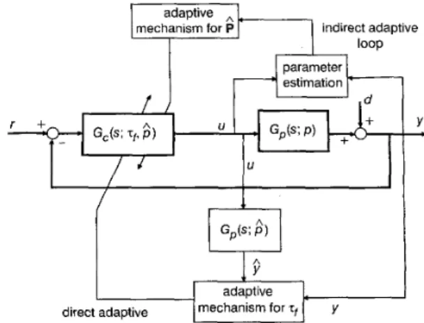
5 A dual adaptive loop (DAL) scheme for

adaptive control

Section 3 addressed adaptive control by adaptively changing zp By such an adaptation, the system will have a floating zfand obviously the system cannot have as good a performance as that expected from the nominal system. As shown in Section 4, the indirect type of adaptive control alone cannot guarantee robust stability during the period of identification. However, since the changed parameters have been identified and updated, the performance of the system can be resumed later on. In order to enjoy the advantages of both types of control, a DAL system for adaptive control is thus considered. In this DAL system, the indirect and direct adaptive mechanisms are implemented through two different loops. The overall system is shown in Fig. 2 and is implemented according to the following procedure.

1. Whenever a set-point change is made to the system, the direct adaptive loop adjusts the value of zf according to (16) and (17) in Section 3 to ensure robustness of stability and performance.

2. At the same time, the indirect loop starts to collect input

64

indirect adaptive

/

loop

Fig. 2 Dual adaptive loop (DAL) system for robust and adaptive control

and output data to estimate the system parameters. 3. When the computed matrix, @, becomes full rank, identification computation starts along with increasing N .

On-line estimation stops either when the parameter vector P converges, or when the information contents of the matrix @ become insufficient. In the latter case, the minimum singular value of @ will smaller than an assigned limiting constant. In general, this small constant is taken as small as 1.0 x

4. The parameters of the controller are updated according to the identified nominal model, and the direct loop starts again using (6).

The weakness of the indirect adaptive loop is made up for by the direct adaptive loop, which guarantees stability of the system even when the resulting nominal model is not correct. The value of zf of the direct loop is changed back to its nominal designed value when on-line identification of the indirect loop is completed. As a result,

zf

will not drift if no further parameter changes occur.

6 Example-robust and adaptive PID control

systems

Starting with a nominal model of (5) and using the IMC design to find C, the resulting G, is a PID controller of the following form:

where the parameters are given as those of (7).

It is clear that the parameters in the PID controllers are functions of both zjand those parameters in Gp. Therefore, by applying the adaptive mechanisms, the controller can be tuned- on-line to obtain a self-tuning robust and adaptive control system. This self-tuned system can alleviate the difficulties and drawbacks pointed out by Chia and Cleve- land [ 7 ] .

The proposed DAL control system is demonstrated using the following examples, which use PID controllers.

6. I Control with the proposed direct adaptive system

Example 1 : Assume that the real plant and the nominal model are

e-' (30)

1.5 22 9 G,(s) =

-

2s

+

1 s2

+

30s

+

229

(6)

1.4 5 s f 1

G,(s)

= - e-”

The above dynamic systems are simulated using the numerical Runge-Kutta method for integrating differential equations. The integration time sub-interval is taken as 0.005. The correct first-order model for G,(s) is found to be:

1‘5 e-1.15s

G,(s) = _ _

2 s + 1 (32)

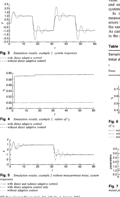
Because the given model has a modelling error compared with G;(s), the actual response has extensive oscillations as shown in Fig. 3.

If the direct loop is incorporated with the original IMC controller, ?f is changed as shown in Fig. 4. Then the oscillations are attenuated. In this case, the modelling error is within reasonable limits, thus, after incorporating the direct adaptive loop, the performance is acceptable. 6.2 Control with the DAL adaptive system Sometimes, deviations of the nominal parameters from the true ones are too large for the performance to be acceptable. Indirect adaptation via the system identification of

2.5 2.0[ -0 5 -1 0

T

-1 5

--L

, . ! f i : -2.0 -2.5 I 0 10 20 30 40 50 60 t Fig. 3

__ with direct adaptive control

- _ _ _ without direct adaptive control

Simulation results, example 1, system responses

0.60

0.58r

0.56 “05411 0.52 0.50 ~ - ...- - ... ~ ... 0.48 I 0 10 20 30 40 50 60 t Fig. 4

__ with direct adaptive control

_ _ _ _

without direct adaptive control

Simulution results, example 1. values of zf

I I I I I I 0 10 20 30 40 50 60 t -3

’

Fig. 5 responses

__ with direct and indirect adaptive control with direct adaptive control only ... without adaptive control

Simulation results, example 2 without measurement noise, system

parameter sensitivity approach should be used in addition to a directed adaptation loop to obtain better performance. In the following, example 2 illustrates the advantage of adaptive control with dual loops over that of a direct adaptive loop alone.

Example 2: Consider the same real plant as in example 1, but that the nominal model with modelling error is given as

1.2 3s

+

1

G,(s) =

-

e-’ (33) Fig. 5 shows the responses of the three systems to step set-point changes, with the simulation parameters shown in Table 1.

Because this model has a large modelling error compared with G;, the IMC control alone gives even greater oscillations than those of Example 1 at the output. Then, a direct adaptive loop is added and the zf

is adapted as shown in Fig. 6. Although the oscillations are attenuated, the performance is still unacceptable. Finally, the indirect adaptive loop is incorporated along with the direct adaptive loop. Fig. 7 shows, the estimation results of the parameters during the identification. The system takes about five units of time to finish the recursive identification. This can be seen by the sudden change of zf to a new value. The second step set-point change occurs at t=30, and since the modelling errors have been corrected, the system at this point shows extremely good performance.

In the previous simulations, it is assumed that no measuring errors exists in the sampled data. If random errors having a normal distribution N(0, 0.1) are added to the sampled output, the results are as shown in Figs. 8-10. As can be seen, the DAL adaptive scheme still works well in the presence of measurement noise.

Table 1: Simulation parameters used in example 2 Sampling i nterva I

Initial data length 20 points

c 0.05 %top 0.001 0.1 time unit - - - - - - p+

--,----I----

;;1,

I I

,

0 5 0 4 0 10 20 30 40 50 60 t Fig. 6 o f

~ with direct and indirect adaptive control

_ _ with direct adaptive control only without adaptive control

Simulation results, example 2 without measurement noise, values

6

2.5 z

n

kp n a 1.0

-

~~ V.“ 0 10 20 30 40 50 60 t Fig. 7

mated plant parameters during identiJication

Simulation results, example 2 without measurement noise, esti-

(7)

-2 -3 I I I I I I 10 20 30 40 50 60 t Fig. 8 responses

with direct adaptive control only

. . . without adaptive control

Simulation results, example 2 with measurement noise, system

I I I I I I 10 20 30 40 50 60 0.4 I t Fig. 9 7f

with direct adaptive control only

... without adaptive control

Simulation results, example 2 with measurement noise, values of

3.5r 1 .o e 0.5 I I I I I I 0 10 20 30 40 50 60 t Fig. 10

mated plant parameters during identijication

Simulation results, example 2 with measurement noise, esti-

7 Concluding remarks

A DAL system for self-tuning adaptive control has been presented. The main advantages of this design include:

1. The system changes its controller parameters through normal closed-loop operation.

2. The system can achieve tighter control performance via a self-tuning procedure in the indirect adaptive loop and can achieve robust stability via the direct adaptive loop.

Simulation results show that the proposed DAL system can be used effectively on-line to auto-tune or self-tune PID controllers. 8 1 2 3 4 5 6 7 8 66 References

LANDAU, I.D.: ‘From robust control to adaptive control’, Control Eng. Pract., 1999, 7 , p p . 1113-1124

SKOGESTAD, S., and POSTLETHWAITE, I.: ‘Multivariate feedback control-analysis and design’ (John Wiley & Sons, 1996)

BHATTACHARYYA, S.P., CHAPELLAT, H., and KEEL, L.H.: ‘Robust

control-the parametric approach’ (Prentice-Hall, 1995)

SEBORG, D.E., and EDGAR, T.F.: ‘Adaptive control strategies for process control: a survey’, AICHE J , 1986,32, (6), pp. 881-913

KRSTIC, M., KANELLAKOPOULOS, I., and KOKOTOVIC, P.:

‘Nonlinear and adaptive control design’ (John Wiley & Sons, 1995) IOANNOU, P.A., and SUN, J.: ‘Robust adaptive control’ (Prentice-Hall,

1996)

CHIA, T.C., and CLEVELAND, 0.: ‘Some basic approaches for self- tuning controllers’, Control Eng., 1992, pp. 49-52

ASTROM, K.J., and WITTENMARK, B.: ‘Adaptive control’ (Addison- Wesley, 1989) 9 10 11 12 13 14 15 16 17 18 19 20 9

NARENDRA, K.S., and ANNASWARY, A.M.: ‘Stable adaptive

systems’ (Prentice-Hall, 1989)

ORTEGA, R., and TANG, Y.: ‘Robustness of adaptive controllers-a survey’, Automatica, 1989, 25, pp. 651-677

SASTRY, S., and BODSON, M.: ‘Adaptive control: stability, conver- gence, and robustness’ (Prentice-Hall, 1989)

BUTLER, H.: ‘Model reference adaptive control: from theory to practice’ (Prentice-Hall, 1992)

RIVERA, D.E., MORARI, M., and SKOGESTAD, S.: ‘lntemal model control 4. PID controller design’, Int. Eng. Chem. Process Design Dev., BISWAS, K.K., and SINGH, G.: ‘Identification of stochastic time delay systems’, IEEE. Trans. Autom. Control, 1978, 23, pp. 504-505 GERRY, J.P., VOGEL, E.F., and EDGAR, T.F.: ‘Adaptive control of a pilot scale distillation column’. Proceedings of American Control Conference, 1983, San Francisco, USA, pp, 819-824

CHIEN, I.L., SEBORG, D.E., and MELLICHAMP, D.A.: ‘Self-tuning controller for systems with unknown or varying time delays’. Proceed- ings of American Control Conference, 1984, San Diego, USA, pp. 905- 912

LAMMERS, H.C., and VERBRUGGEN, H.B.: ‘Simple self-tuning control of processes with a slowly varying time‘ delay’. IEE Control Conference, 1985, Cambridge, UK, pp. 393-398

HUANG, H.P., and CHENG, C.C.: ‘Transfer function matrix identification of MIMO dynamic systems’, Chin. I. Ch. E., 1989, 20, (l), pp. 31-39

LJUNG, L.: ‘System identification-theory for the user’ (Prentice-Hall, 1999,2nd edn.)

HUANG, H.P., and WANG, G.B.: ‘Control and estimation for perturbed nonlinear process with dead-time’, Chem. Eng. Commun., 1992, 117, 1986, 25, pp. 252-265

pp. 117-141

Appendix

9.

I

Proof of property 1

For a step change of set-point, we have P ( S ) = 11s and

(34) Because Gc(s) is obtained by (6) and y ( s ) is obtained by

it is easy to see that

k ? y ( t =

e,)

= JL ?a

(3 5)

Furthermore, by the definitions of the PID parameters given in (7), the result is obtained as

k 7 j ( t =

e,)

= P

Tf kP

(37)

9.2 Proof of property 2 According to the definition of l ,

(3 8) and because the steady state gains Gp and

G,

are of the same sign, it is found that

l(O)F(O) 2 -1 (39)

Il(jo)F(jo)l < co as o ++ 00 (40) and

According to (39), the Nyquist map of G+Fl always starts from a point on the real axis to the right of (-1, 0). It can then be shown that for any l ( s ) , there exists a value, such that the Nyquist map of G + F l ( j o ) will never cross the real axis at a point to the left of (- 1, 0) for all

Zf 2 ??I,.

(8)

Since I Z ; + I = l V o E [ O , 0 O ) (41) we have

l%o)l

(42)

JGZj

I

G+Fe(Jw>

I

i

I

e ( j 0 )

I I

F ( j w )

I

=

Thus, for a given

e@),

assuming that the maximum value of

throughout w E [0, 00) occurs at w = coo, it is clear that

Here, is the maximum of

I

lju

1

for V u E [0, 00). For

1, the above inequality holds for,each

zf?

0. In the case where

2

> 1, there is a value for zfmrn of the following, i.e.

(44)

Here, for any ?f>

:Fin,

the following result holds true:

Thus, it ,can be concluded that, for each

zf

which is greater than zfmrn obtained by (44), the system can be stabilised

with the IMC-PID controller.