Reinforcement hybrid evolutionary learning for recurrent wavelet-based neurofuzzy systems

Abstract—This paper proposes a recurrent wavelet-based

neurofuzzy system (RWNFS) with the reinforcement hybrid evolutionary learning algorithm (R-HELA) for solving various control problems. The proposed R-HELA combines the compact genetic algorithm (CGA), and the modified variable-length genetic algorithm (MVGA) performs the structure/parameter learning for dynamically constructing the RWNFS. That is, both the number of rules and the adjustment of parameters in the RWNFS are designed concurrently by the R-HELA. In the R-HELA, indi-viduals of the same length constitute the same group. There are multiple groups in a population. The evolution of a population consists of three major operations: group reproduction using the compact genetic algorithm, variable two-part crossover, and vari-able two-part mutation. Illustrative examples were conducted to show the performance and applicability of the proposed R-HELA method.

Index Terms—Control, genetic algorithms, neurofuzzy system,

recurrent network, reinforcement learning.

I. INTRODUCTION

I

N recent years, a fuzzy system used for control problems has become a popular research topic [1]–[10]. The reason is that classical control theory usually requires a mathematical model for designing controllers. Inaccurate mathematical modeling of plants usually degrades the performance of the controllers, espe-cially for nonlinear and complex problems [11]–[14]. A fuzzy system consists of a set of fuzzy if-then rules. By convention, the selection of fuzzy if-then rules often relies on a substan-tial amount of heuristic observations to express knowledge of proper strategies. Obviously, it is difficult for human experts to examine all the input–output data from a complex system to find the proper rules for a fuzzy system. To cope with this difficulty, several approaches to generating if-then rules from numerical data have been proposed [6], [8], [11], [54].These methods were developed for supervised learning; that is, the correct “target” output values are given for each input pattern to guide the network’s learning. Lin and Chin [11] used mech-anisms of rules/neurons update based on errors, while evolving fuzzy rule-based (eR) models [54] used the informative poten-tial of the new data sample as a trigger to update the rule-base.

Manuscript received April 14, 2005; revised February 16, 2006 and May 16, 2006. This work was supported by the National Science Council, R.O.C., under Grant NSC95-2221-E-324-028.

C.-J. Lin is with the Department of Computer Science and Information Engi-neering, Chaoyang University of Technology, Taichung County 41349, Taiwan, R.O.C. (e-mail: cjlin@mail.cyut.edu.tw).

Y.-C. Hsu is with the Department of Electrical and Control Engineering, Na-tional Chiao-Tung University, Taiwan, R.O.C. (e-mail: ericbogi2001@yahoo. com.tw).

Digital Object Identifier 10.1109/TFUZZ.2006.889920

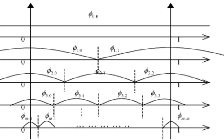
Fig. 1. Wavelet bases are overcompleted and compactly supported.

The most well-known supervised learning algorithm is back-propagation (BP) [3], [6]–[8]. It is a powerful training technique that can be applied to networks. Since the steepest descent tech-nique is used in BP training to minimize the error function, the algorithm may reach the local minima very fast and never find the global solution. In addition, the performance of BP training depends on the initial values of the system parameter. For dif-ferent network topologies, one has to derive new mathematical expressions for each network layer. If precise training data can be easily obtained, the supervised learning algorithm may be ef-ficient in many applications. For some real-world applications, precise training data are usually difficult and expensive to ob-tain. For this reason, there has been a growing interest in rein-forcement learning problems [15]–[17]. For the reinrein-forcement learning problems, training data are very rough and coarse, and they are only “evaluative” when compared with the “instructive” feedback in the supervised learning problem.

Recently, many evolutionary algorithms, programming types, and strategies, such as the genetic algorithm (GA) [18], genetic programming [19], evolutionary programming [20], and evolu-tion strategies [21], have been proposed. Since they are heuristic and stochastic, they are less likely to get stuck at the local min-imum. They are based on populations made up of individuals with specific behaviors similar to certain biological phenomena. These common characteristics have led to the development of evolutionary computation as an increasingly important field.

The evolutionary fuzzy model generates a fuzzy system au-tomatically by incorporating evolutionary learning procedures [22]–[32], such as the GA, which is a well-known procedure. Several genetic fuzzy models, that is, fuzzy models augmented by a learning process based on GAs, have been proposed [22]–[29]. In [22], Karr applied GAs to the design of the 1063-6706/$25.00 © 2007 IEEE

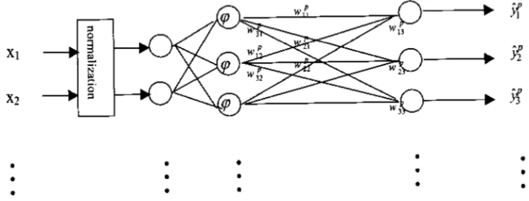
Fig. 2. Schematic diagram of the WNN.

membership functions of a fuzzy controller, with the fuzzy rule set assigned in advance. Since the membership functions and rule sets are codependent, simultaneous design of these two approaches would be a more appropriate methodology.

Based on this concept, many researchers have applied GAs to optimize both the parameters of the membership functions and the rule sets [23]–[25], [53]. Ishibuchi et al. [53] proposed a genetic-algorithm-based method for selecting a small number of significant fuzzy if-then rules to construct a compact fuzzy classification system with high classification power. The rule se-lection problem is formulated as a combinatorial optimization problem with two objectives: to maximize the number of cor-rectly classified patterns and to minimize the number of fuzzy if-then rules. Lin and Jou [27] proposed GA-based fuzzy rein-forcement learning to control magnetic bearing systems. In [28], Juang et al. proposed using genetic reinforcement learning in the design of fuzzy controllers. The GA adopted in [28] was based upon traditional symbiotic evolution, which, when applied to fuzzy controller design, complements the local mapping prop-erty of a fuzzy rule. However, the aforementioned approaches may require one or both of the following: 1) the numbers of fuzzy rules have to be assigned in advance and 2) the lengths of the chromosomes in the population must be the same.

Recently, several researchers proposed new genetic algo-rithms for solving the above-mentioned problems. In [29], Bandyopadhyay et al. used the variable-length genetic algo-rithm (VGA) that allows for different lengths of chromosomes in the population. Carse et al. [30] used the genetic algorithm [29] to evolve fuzzy rule based controllers. In [31], Tang proposed a hierarchical genetic algorithm, which enables the optimization of a fuzzy system design for a particular appli-cation. Juang [32] proposed the CQGAF to simultaneously design the number of fuzzy rules and free parameters in a fuzzy system.

In this paper, we proposed a new hybrid evolutionary learning algorithm to enhance the VGA [29]. The performance of the number of fuzzy rules in the VGA has not been evaluated, so that the best group that has the same length of chromosomes cannot be reproduced many times for each generation. In this paper, we use the elite-based reproduction strategy to keep the best group that has chromosomes of the same length. Therefore, the best group can be reproduced many times for each genera-tion. The elite-based reproduction strategy is similar to the

ma-turing phenomenon in society, where individuals become more suited to the environment as they acquire more knowledge of their surroundings.

In this paper, we present a recurrent wavelet-based neuro-fuzzy system (RWNFS) with the reinforcement hybrid evolu-tionary learning algorithm (R-HELA). The proposed R-HELA automatically determines the number of fuzzy rules and pro-cesses the variable-length chromosomes. The length of each in-dividual denotes the total number of genes in that inin-dividual. The initial length of one individual may be different from an-other individual, depending on the total number of rules encoded in it. Individuals with an equal number of rules constitute the same group. Thus, initially there are several groups in a popu-lation. We use the elite-based reproduction strategy to keep the best group. Therefore, the best group can be reproduced many times for each generation. The reinforcement signal from the environment is used as a fitness function for the R-HELA. That is, we formulate the number of time steps before failure occurs as the fitness function. In this way, the R-HELA can evaluate the candidate solutions for the parameters of the RWNFS model.

The advantages of the proposed R-HELA method are sum-marized as follows.

1) It determines the number of fuzzy rules and tunes the free parameters of the RWNFS model in a highly autonomous way. Thus, users need not give it any a priori knowledge or even any initial information on these parameters.

2) It is applicable to chromosomes of different lengths. 3) It does not require precise training data for setting the

pa-rameters of the RWNFS model.

4) It performs better and converges more quickly than some traditional genetic methods.

This paper is organized as follows. Section II introduces the RWNFS. The proposed HELA is described in Section III. Section IV introduces the reinforcement hybrid evolution learning algorithms used for constructing the RWNFS model. Section V presents the simulation results. The conclusions are given in the last section.

II. STRUCTURE OF ARECURRENTWAVELET-BASED NEUROFUZZYSYSTEM

This section introduces the structure of an RWNFS model. For traditional TSK-type fuzzy systems [5]–[7], the conse-quence of each rule is a function of the input linguistic variable.

Fig. 3. Schematic diagram of RWNFS model.

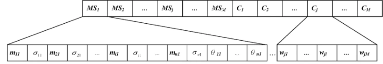
Fig. 4. Coding the adjustable parameters of a RWNFS into a chromosome in the MVGA.

Fig. 5. Coding the probability vector into the building blocks in the CGA.

A widely adopted function is a linear combination of input variables plus a constant term. This paper adopts a nonlinear combination of input variables [i.e., wavelet neural network (WNN)]. Each fuzzy rule corresponds to a sub-WNN consisting

of single-scaling wavelets [33]. We adopt the nonorthogonal and compact wavelet functions as the node function (wavelet bases).

A. Description of Wavelet Bases and Wavelet Neural Networks

A set of wavelet bases is a suitable tool for representing nonlinearity effectively. These orthogonal wavelets are infinite, continuous, and differentiable. The support of these wavelets is . Daubechies [34] presented wavelet bases, which are compactly supported but not infinitely supported.

Fig. 6. The flowchart of the parameter learning in the HELA.

Daubechies proposed using a simple wavelet neural network, which exhibits a much higher ability to generalize and a much shorter learning time, rather than a three-layered feedforward neural network. This study adopts the nonorthogonal and com-pactly supported functions in the finite range as wavelet bases. Fig. 1 shows the shape and position of the wavelet bases. All the wavelet bases are allocated over the normalized range [0, 1] in the variable space.

Neural networks employing wavelet neurons are referred to as wavelet neural networks. Fig. 2 shows a novel type of wavelet neural network model [35]. Consider input

vectors and output vectors

. This model is obtained by re-placing a sigmoidal activation function with single-scaling wavelets [35]. The wavelet neural networks are characterized by weights and wavelet bases. Each linear synaptic weight of the wavelet bases is adjustable by learning. Notably, the ordinary wavelet neural network model applications are often useful for normalizing the input vectors into the interval [0, 1]. The functions that are used to input vectors to fire up the wavelet interval are then calculated. The value is obtained as shown in the equation at the bottom of the page,

where

(1) The above equation formulates the nonorthogonal wavelets in a finite range, where denotes a shifting parameter, the maximum value of which equals the corresponding scaling parameter ; and denotes the number of wavelet bases, which equals the number of existing fuzzy rules in the RWNFS model. In the RWNFS model, wavelet bases do not exist in the initial state. The amount of wavelet bases generated by the online learning algorithm is consistent between wavelet bases and fuzzy rules. The online learning algorithm is detailed in Section III. A crisp value can be obtained as follows:

(2) where is the number of input dimensions. The final output of the wavelet neural networks is

(3)

Fig. 7. The learning diagram of the proposed ERS method.

where denotes the local output of the WNN for output and the th rule; and the link weight is the output action strength associated with the th output, th rule, and th .

B. Structure of the RWNFS Model

This section introduces the structure of the RWNFS model shown in Fig. 3. For TSK-type fuzzy networks [5]–[7], the con-sequence of each rule is a linear function of input linguistic vari-ables. A widely adopted function is a linear combination of input variables plus a constant term. This study adopts a nonlinear combination of input variables (i.e., WNN). Each fuzzy rule cor-responds to a sub-WNN consisting of single-scaling wavelets

[33]. A novel RWNFS model is composed of fuzzy rules that can be presented in the following general form:

is and is and and is

Then

and

..

Fig. 8. The pseudocode of the ERS.

where denotes the th rule; is the

network input pattern plus the

tem-poral term for the linguistic term of the precondition part ; and the local WNN model outputs and are calculated for outputs and and rule

.

Next, the signal propagation is indicated, along with the op-eration functions of the nodes in each layer. In the following description, denotes the th input of a node in the th layer and denotes the th node output in layer .

Layer 1 nodes just transmit input signals to the next layer directly, that is

(5)

where . Each premise part of the

th rule (a set of fuzzy sets) is

described here by a Gaussian-type membership function; that is, the membership value specifying the degree to which an input value belongs to a fuzzy set is determined in layer 2. The Gaussian function is defined by

(6)

where and are the mean and standard deviation, respec-tively. Additionally, the input of this layer for the discrete time

can be denoted by

(7)

where is the feedback weight. Clearly, the input of this layer contains the memory terms , which store the past information of the network. This is the apparent difference be-tween the WFNN [11] and RWNFS models.

In the proposed RWNFS model, the recurrent property is achieved by feeding the output of each membership function back to itself so that each membership value is influenced by its previous value. Although some recurrent neural fuzzy networks have been proposed and applied to dynamic system identification and control, there are still disadvantages to these network structures. In [36], we need to know the order of both the control input and the network output to participate in the autoregressive with exogenous model. We solve this problem by feeding back the output of each membership function. Only the current control input and system state are fed to the network input. The past values can be memorized by using feedback structure. In [37], a global feedback structure is adopted, and the outputs of all rule nodes, the firing strengths, are fed back and summed. In this case, the TRFN model [37] needs more adjustable parameters. However, we will show by simulation that the proposed RWNFS model achieves better performance and requires a smaller number of tuning parameters than the model in [37].

In layer 3, defining the number and the locations of the mem-bership functions leads to the partition of the premise space

. The collection of fuzzy sets pertaining to the premise part of formulates a fuzzy region in that can be regarded as a multidi-mensional fuzzy set whose membership function is determined by

(8)

Fig. 9. The variable two-part crossover operation in the HELA.

Fig. 10. The variable two-part mutation operation in the HELA.

Layer 4 only receives the signal from the output of the wavelet neural network model for an output and the th rule. The mathematical function of each node is

(9) The final output of the model is calcu-lated in layer 5. The output node together with recalcu-lated links acts as a defuzzifier. The mathematical function is shown in

(10) where denotes the output of the local model of the WNN model for an output and the th rule, is the output of layer 3, and is the th output of the RWNFS model.

III. A HYBRIDEVOLUTIONARYLEARNINGALGORITHM (HELA)

This section introduces the proposed HELA. Recently, many efforts to enhance the traditional GAs have been made [38]. Among them, one category focuses on modifying the structure of a population or the role an individual plays in it [39]–[41], such as the distributed GA [39], the cellular GA [40], and the symbiotic GA [41].

In a traditional evolution algorithm, the number of rules in a model must be predefined. Our proposed HELA combines

the compact genetic algorithm (CGA) and the modified vari-able-length genetic algorithm (MVGA). In the MVGA, the ini-tial length of each individual may be different from each other, depending on the total number of rules encoded in it. Thus, we do not need to predefine the number of rules. In this paper, indi-viduals with an equal number of rules constitute the same group. Initially, there are several groups in a population. Not following the traditional VGA notation, Bandyopadhyay et al. [29] used “#” to mean “does not care.” In this paper, we adopt the variable two-part crossover (VTC) and the variable two-part mutation (VTM) to make the traditional crossover and mutation opera-tors applicable to different lengths of chromosomes. Therefore, we do not use “#” to mean “does not care” in the VTC and the VTM.

In this paper, we divide a chromosome into two parts. The first part of the chromosome gives the antecedent parameters of a RWNFS model, while the second part of the chromosome gives the consequent parameters of a RWNFS model. Each part of a chromosome can be performed using the VTC on the overlap-ping genes of two chromosomes. In the traditional VGA, Bandy-opadhyay et al. [29] only evaluated the performance of each chromosome in a population. The performance of the number of rules was not evaluated in [29].

In this paper, we use the elite-based reproduction strategy to keep the best group that has chromosomes of the same length. Therefore, the best group can be reproduced many times for each generation. The elite-based reproduction strategy is similar to the maturing phenomenon in society, in which individuals become more suited to the environment as they acquire more knowledge of their surroundings.

In the proposed HELA method, we adopt the CGA [42] to carry out the elite-based reproduction strategy. The CGA represents a population as a probability distribution over the set of solutions and is operationally equivalent to the order-one

Fig. 11. Schematic diagram of the R-HELA for the RWNFS model.

Fig. 12. Flowchart of the R-HELA method.

behavior of the simple GA [43]. The advantage of the CGA is that it processes each gene independently and requires less memory than the normal GA. The building blocks (BBs) in the CGA represent the suitable lengths of the chromosomes, and the CGA reproduces the chromosomes according to the BBs.

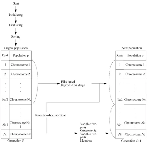
The coding scheme consists of the coding done by the MVGA and the CGA. The MVGA codes the adjustable parameters of a RWNFS model into a chromosome, as shown in Fig. 4, where represents the parameters of the antecedent of the th rule in the RENFN and represents the parameters of the conse-quent of the th rule. In Fig. 5, the CGA codes the probability vector into the BBs, where each probability vector represents the suitability of the rules of a RWNFS model. In the CGA, we must predefine the maximum number of rules and the min-imum number of rules to prevent generating the number of fuzzy rules beyond a certain bound (i.e., ).

The learning process of the HELA involves six major oper-ators: initializing, evaluating, sorting, elite-based reproduction strategy, variable two-part crossover, and variable two-part mu-tation. Fig. 6 shows the flowchart of the learning process. The whole learning process is described step-by-step as follows.

a) Initializing: The initializing step sets the initial values in the MVGA and the CGA. In the MVGA, individuals are initially randomly generated to construct a population. In order to keep the same number of rules in an RWNFS model, the number of rules for each chromosome needs to be generated chromosomes. That is, we predefine the number of chromosomes generated for each group .

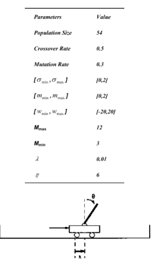
TABLE I

THEINITIALPARAMETERSBEFORETRAINING

Fig. 13. The cart-pole balancing system.

Therefore, the population size is set to

1 . In the CGA, the probability vectors of the BBs are set to 0.5 initially.

b) Evaluating: The evaluating step evaluates each chromo-some in a population. The goal of the R-HELA method is to maximize the fitness value. The higher a fitness value, the better the fitness. The fitness function is used by a re-inforcement signal in (16) that we will introduce in next section.

c) Sorting: After the evaluating step, we sort the chromo-somes in the population. After the whole population is sorted, we sort the chromosomes in each group in the top half of population. The sorting step can help us to perform the reproduction step because we can keep the best chro-mosome in each group. After sorting the chrochro-mosomes in the population, the algorithm goes to next step.

d) Elite-Based Reproduction Strategy (ERS): Reproduction is a process in which individual strings are copied ac-cording to their fitness value. A fitness value is assigned to each individual using (16). The goal of the R-HELA method is to maximize the fitness value. The higher a fit-ness value, the better the fitfit-ness. In this paper, we use an ERS to mimic the maturation phenomenon in society, in

Fig. 14. The performance of (a) the R-HELA method, (b) the R-SE method [28], and (c) the R-GA method [22] on the cart-pole balancing system.

which individuals become more suited to the environment as they acquire more knowledge of their surroundings. The CGA is used here to carry out the ERS. The CGA represents the population as a probability distribution over the set of solutions and is operationally equivalent to the order-one behavior of the simple GA. The CGA uses the BBs to represent the suitable lengths of the chromosomes and reproduces the chromosomes according to the prob-ability vector in the BBs. The best performing individ-uals in the top half of each population are used to perform

Fig. 15. The probability vectors of the ERS step in the proposed R-HELA.

the ERS. According to the results of the ERS, using the crossover and the mutation operations generates the other half of the individuals. The learning diagram of the pro-posed ERS method is shown in Fig. 7. After the ERS, the suitable length of chromosomes will be preserved and the unsuitable length of chromosomes will be removed. De-tails of the ERS are shown below.

Step 1) Update the probability vectors of the BBs ac-cording to the following equations:

if otherwise (10) where (11) Total (12) Total (13)

where is the probability vector in the BBs and represents the suitable chromosome in the group with rules in a population; is a threshold value we predefine; Avg represents the average fitness value in the whole population; Nc is the population size; is the th group size; fit is the fitness value of the th chromosome in all Nc populations; fit is the fitness value of the th chromosome in the th group; and is the best fitness value [maximum value of (16)] in the th group. As shown in (10), if

, then the suitable chromosomes in the th group should be increased. On the other hand,

Fig. 16. Angular deviation of the pole by a trained (a) R-HELA method, (b) R-SE method [28], and (c) R-GA method [22].

if , then the suitable chromo-somes in the th group should be decreased. Equation (13) represents the sum of the fitness values of the chromosomes in the th group.

Step 2) Determine the reproduction number according to the probability vectors of the BBs as follows:

Total

where (14)

Total (15)

where represents the population size, is the recorder, and a chromosome has rules for constructing an RWNFS.

Step 3) After Step 2), the reproduction number of each group in the top half of a population is obtained. Then we generate chromosomes in each group using the roulette-wheel selection method [44].

Step 4) If any probability vector in BBs reaches 1, then stop the ERS and set the probability vector to 1 for all groups with the same number of rules, according to Step 2). The lacks of the chromo-somes are generated randomly. To replace the ERS step, we use the roulette-wheel selection method [44]—a simulated roulette is spun—for this reproduction process. The pseudocode for the ERS is shown in Fig. 8.

e) Variable Two-Part Crossover: Although the ERS opera-tion can search for the best existing individuals, it does not create any new individuals. In nature, an offspring has two parents and inherits genes from both. The main op-erator working on the parents is the crossover opop-erator, the operation of which occurs for a selected pair with a crossover rate.

In this paper, we propose using the VTC to perform the crossover operation. In the VTC, the parents are selected from the enhanced elites using the roulette-wheel selec-tion method [44]. The two parents may be selected from the same or different groups. Performing crossover on the selected parents creates the offspring. Since the par-ents may be of different lengths, we must avoid misalign-ment of individuals in the crossover operation. There-fore, a variable two-part crossover is proposed to solve this problem. The first part of the chromosome gives the antecedent parameters of an RWNFS model while the second part of the chromosome gives the consequent pa-rameters of an RWNFS model. The two-point crossover is adopted in each part of the chromosome. Thus, new individuals are created by exchanging the site’s values between the selected sites of the parents’ individuals. To avoid the misalignment of individuals in the crossover op-eration, in the VTC, the selection of the crossover points in each part will not exceed the shortest length chromo-some of two parents. Two individuals of different lengths resulting from the use of the variable two-part crossover operation are shown in Fig. 9. represents the param-eters of the antecedent part of the th rule in the RENFN; represents the parameters of the consequent of the th rule in the RENFN; and M k is the number of fuzzy rules

the mutation operation. The proposed VTM is different from the traditional mutation and is applicable to chro-mosomes of different lengths. The first and second parts of the chromosome are the same as the crossover opera-tion. In each part of a chromosome, uniform mutation is adopted, and the mutated gene is drawn randomly from the domain of the corresponding variable. The VTM op-eration for each individual is shown in Fig. 10.

After the above-mentioned operations are carried out, the problem of how groups are to be constituted by the most suitable number of rules will be solved. The number of elites in other groups will decrease, and most of them will become zero (in most cases, there will be no elites). That is, our method indeed can eliminate unsuitable groups and rules.

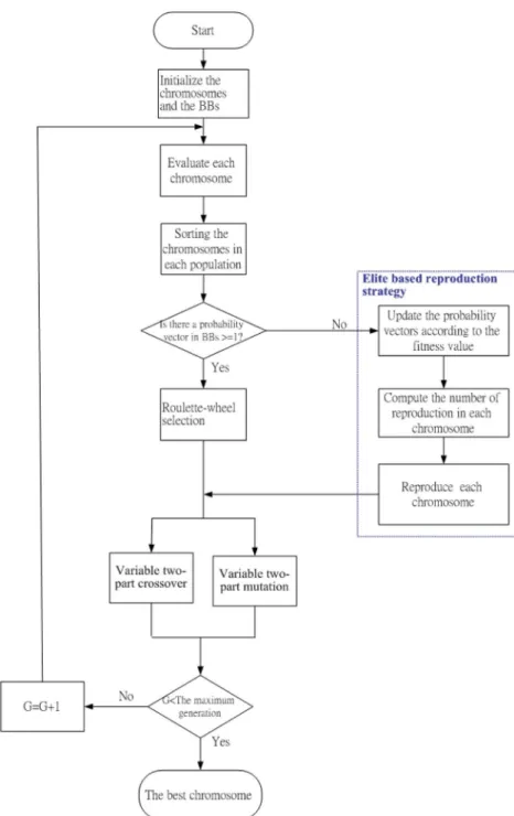
IV. REINFORCEMENTLEARNING FOR ANRWNFS MODEL Unlike the supervised learning problem, in which the cor-rect “target” output values are given for each input pattern, the reinforcement learning problem has only very simple “evalua-tive” or “critical” information, rather than “instruc“evalua-tive” infor-mation, available for learning. In the extreme case, there is only a single bit of information to indicate whether the output is right or wrong. Fig. 11 shows the R-HELA. Its training environment interacts with reinforcement learning problems. In this paper, the reinforcement signal indicates whether a success or a failure occurs.

As shown in Fig. 11, the proposed R-HELA consists of a RWNFS model, which acts as the control network that de-termines the proper action to take according to the current input vector (environment state). The structure of the proposed R-HELA is different from the actor-critic architecture of Barto

et al. [15], which consists of a control network and a critic

network. The input to the RWNFS model is the state of a plant, and the output is a control action of the state, denoted by . The only available feedback is a reinforcement signal that notifies the RWNFS model only when a failure occurs.

An accumulator plays a role which is a relative performance measure, as shown in Fig. 11. It accumulates the number of time steps before a failure occurs. In this paper, the feedback takes the form of an accumulator that determines how long the exper-iment is still a “success”; this is used as a relative measure of the fitness of the proposed R-HELA method. That is, the accumu-lator will indicate the “fitness” of the current RWNFS model. The key to the R-HELA is formulating a number of time steps before failure occurs and using this formulation as the fitness function for the R-HELA method. It will be observed that the advantage of the proposed R-HELA method is that it can meet global optimization capability.

Fig. 12 shows the flowchart of the R-HELA method. The pro-posed R-HELA method runs in a feed-forward fashion to con-trol the environment (plant) until a failure occurs. Our relative measure of the fitness function takes the form of an accumulator that determines how long the experiment is a “success.” In this way, according to a defined fitness function, a fitness value is as-signed to each string in the population where a high fitness value means a good fit. In this paper, we use a number of time steps before failure occurs to define the fitness function. The goal of the R-HELA method is to maximize the fitness value. The fit-ness function is defined by

Fitness Value TIME-STEP (16)

where TIME-STEP represents how long the experiment is a “success” with the th population. Equation (16) reflects the fact that long-time steps before failure occurs (to keep the de-sired control goal longer) means a higher fitness of the R-HELA method.

V. ILLUSTRATIVEEXAMPLES

In this section, we compare the performance of the RWNFS model using the R-HELA method with some existing models for two applications. The first simulation was performed to bal-ance the cart-pole system that was described in [45]. The second simulation was performed to balance the ball and beam system that was described in [47]. The initial parameters for the two simulations are given in Table I. The initial parameters were de-termined by practical experimentation or trial-and-error tests.

Example 1: Control of a Cart-Pole Balancing System: In

this example, we apply the R-HELA method to the classic con-trol problem of a cart-pole balancing. This problem is often used as an example of inherently unstable and dynamic sys-tems to demonstrate both modern and the classic control tech-niques [45]–[47], or the reinforcement learning schemes [27], [28], [48], and is now used as a control benchmark. As shown in Fig. 13, the cart-pole balancing problem is the problem of learning how to balance an upright pole. The bottom of the pole is hinged to a cart that travels along a finite-length track to its

TABLE III

THECOMPARISON OFCPU TIME FORVARIOUSEXISTINGMODELS INEXAMPLE1

right or left. Both the cart and the pole can move only in the ver-tical plane; that is, each has only one degree of freedom.

There are four state variables in the system: , the angle of the pole from an upright position (in degrees); , the angular velocity of the pole (in degrees/seconds); , the horizontal po-sition of the cart’s center (in meters); and , the velocity of the cart (in meters/seconds). The only control action is , which is the amount of force (in newtons) applied to the cart to move it toward left or right. The system fails when the pole falls past a certain angle ( 12 is used here) or the cart runs into the bounds of its track (the distance is 2.4 m from the center to each bound of the track). The goal of this control problem is to determine a sequence of forces that is applied to the cart to balance the pole upright. The equations of motion that we used are

(17)

(18)

(19)

(20) where

the length of the pole

kg combined mass of the pole and the cart kg mass of the pole

m/s acceleration due to the gravity (21)

TABLE IV

PERFORMANCECOMPARISON OFTHREEDIFFERENTMETHODS

Fig. 17. The ball and beam system.

where is the coefficient of friction of the cart on the track,

is the coefficient of friction of the pole on the cart, and (s) is the sampling interval.

The constraints on the variables are

m and N. A control

strategy is deemed successful if it can balance a pole for 100 000 time steps.

The four input variables and the output are normalized between zero and one over the following ranges: . The four normalized state variables are used as inputs to the proposed RWNFS model. The coding of a rule in a chromosome is the form in Fig. 4. The values are floating-point numbers assigned using the R-HELA initially. The fitness function in this example is defined in (16) to train the RWNFS model, where (16) represents how long the cart-pole balancing system fails and receives a penalty signal of 1 when the beam deviates beyond a certain angle ( C) and the cart runs into the bounds of its track ( m). In this experiment,

Fig. 18. The performance of (a) the R-HELA method, (b) the R-SE method [28], and (c) the R-GA method [22] on the ball and beam balancing system.

Fig. 19. The probability vectors of the ERS step in the proposed HELA.

the initial values were set to (0, 0, 0, 0). A total of 30 runs were performed. Each run started in the same initial state. Fig. 14(a) shows that the RWNFS model learned on average to balance the pole at the fifty-fourth generation. In this figure, each run represents that largest fitness value in the current generation being selected before the cart-pole balancing system fails. When the R-HELA method was stopped, we chose the best strings in the population in the final generation and tested them on the cart-pole balancing system. Fig. 15 shows the results of the probability vectors in CGA. In this figure, the final average optima number of rules is four. The obtained fuzzy rules of the RWNFS using the R-HELA method are shown as follows:

is and and is and is is and is and is and is Then is and is and is and is Then is and is and is and is Then

Fig. 16(a) shows the angular deviation of the pole when the cart-pole balancing system was controlled by a well-trained RWNFS model starting in the initial state: . The average angular

Fig. 20. Position deviation of the ball by a trained (a) R-HELA method, (b) R-SE method [28], and (c) R-GA method [22].

deviation was 0.01 . The results show that the trained RWNFS model had good control in the cart-pole balancing system.

We also compared the performance of our system with the re-inforcement symbiotic evolution (R-SE) [28] and the reinforce-ment genetic algorithm (R-GA) [22] when they were applied to the same problem. In the R-GA and the R-SE, the population size was set to 200 and the crossover and mutation probabilities were set to 0.5 and 0.3, respectively. Fig. 14(b) and (c) shows that the R-SE and the R-GA methods learned to balance the pole on average at the eightieth and one hundred forty-ninth genera-tions. Fig. 16(b) and (c) shows the angular deviation of the pole when the cart-pole balancing system was controlled by [28] and [22]. The average angular deviation of [28] and [22] models was 0.06 and 0.1 . As shown in Figs. 13 and 15, the control capabil-ities of the trained RWNFS model using the R-HELA are better than [22] and [28] in the cart-pole balancing system.

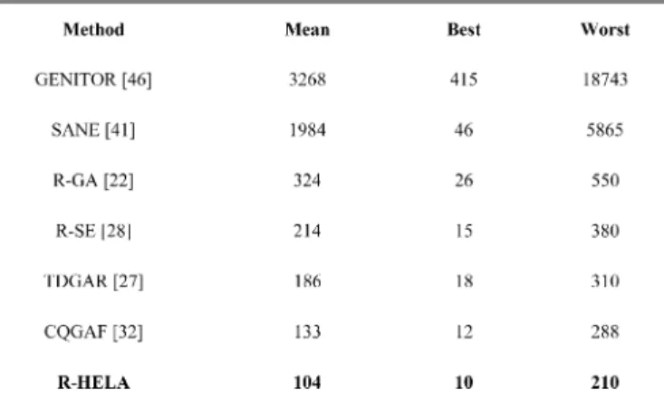
GENITOR [46], SANE [41], TDGAR [27], and CQGAF [32] have been applied to the same control problem; the simu-lation results are listed in Table II. Table II shows the number of pole-balancing trials (which reflects the number of training episodes required). In GENITOR [46], the normal evolution algorithm was used to evolve the weights in a fully connected two-layer neural network, with additional connections from each input unit to the output layer. The network consists of five input units, five hidden units, and one output unit. In SANE [41], the symbiotic evolution algorithm is used to evolve a two-layer neural network with five input units, eight hidden units, and two output units. An individual in the SANE repre-sents a hidden unit with five specified connections to input and output units. The TDGAR [27] learning scheme is a new hybrid GA, which integrates the TD prediction method and the GA to fulfill the reinforcement learning task. The CQGAF [32] fulfills the GA-based fuzzy system design in a reinforcement learning environment where only weak reinforcement signals such as “success” and “failure” are available. As shown in Table II, the proposed R-HELA is feasible and effective. We also compared the CPU times with those of other existing methods [20], [22], [27], [28], [32], [41], and [46]. The results are shown in Table III. In this experiment, we used a Pentium 4 chip with a 1.5 GHz CPU, a 512 MB memory, and the visual C++ 6.0 simulation software. The comparison in Table III shows that our proposed HELA method obtains smaller CPU times than those of other existing models [20], [22], [27], [28], [32], [41], and [46].

To demonstrate the efficiency of the proposed ERS method, three different methods were used in this example: the pro-posed R-HELA method (Type I), the propro-posed R-HELA method without ERS (Type II), and the fixed-length genetic algorithm (Type III). In Type I, the proposed R-HELA method combines the MVGA and the ERS methods. In Type II, the probability vectors are not used to determine the number of fuzzy rules. That is, only the MVGA method is used. In Type III, the number of fuzzy rules is determined by executing a genetic algorithm with a fixed string length for each specification of the number of fuzzy rules, and then the average of the generations is com-puted. Table IV shows the performance comparison of the three methods. As shown in Table IV, our proposed HELA with the ERS method performs better than the other methods.

Example 2: Control of a Ball and Beam System: A ball and

TABLE VI

THECOMPARISON OFCPU TIME FORVARIOUSEXISTINGMODELS INEXAMPLE

2

rotate in a vertical plane when a torque is applied at the center of rotation. The ball is free to roll along the beam. We require that the ball remain in contact with the beam.

The ball and beam system can be written in state space form as

(22)

where is the state of

the system and is the output of the system. The control is the angular acceleration , and the parameters and are chosen in this system. The pur-pose of control is to determine such that the closed-loop system output will converge to zero from different initial con-ditions.

According to the input/output-linearization algorithm [47], the control law is determined as follows: for state ,

com-pute , where

, and the are chosen so that is Hurwitz polynomial. Compute

and ; then .

The four input variables and the output are normalized between zero and one over the following ranges: . The values are floating-point numbers initially assigned using the R-HELA. In the proposed R-HELA method, the fitness func-tion in this example is also defined in (16) to train the RWNFS model, where (16) states how long the ball and beam system fails and receives a penalty signal of 1 when the beam devi-ates beyond a certain angle ( C) and the ball reaches the end of the beam ( m). A total of 30 runs were per-formed. Each run started in the same initial state. Fig. 18(a) shows that the RWNFS model learned on average to balance the ball in the sixty–sixth generation. In this figure, each run results in the largest fitness value in the current generation being se-lected before the ball and beam system fails. After the learning process was stopped, we chose the best string in the popula-tion in the final generapopula-tion and tested it on the ball and beam system. Fig. 19 shows the results of the probability vectors in the ERS. As shown in Fig. 19, the final average optimal number of rules is four. The obtained fuzzy rules of the RWNFS using the R-HELA method are shown as follows:

is and is and is and is Then is and is and is and is Then is and is and is and is Then is and is and is and is Then

Fig. 20(a) shows the position deviation of the ball when the ball and beam system was controlled by the well-trained RWNFS model starting at the initial state:

of the ball decays to zero gradually. The results show that the trained RWNFS model has good control in the ball and beam balancing system.

In this example, as with example 1, we also compared the performance of our method with the R-SE method [28] and the R-GA method [22]. The R-GA and the R-SE methods used the same as those used in example 1. Figs. 18(b) and (c) shows that the R-SE method and the R-GA method learned, on average, to balance the ball in the one hundred ninety-fourth generation and two hundred sixty-eighth generation. Fig. 20(b) and (c) shows the position deviation of the ball when the ball and beam system was controlled by the R-SE and the R-GA methods starting in the initial state . As shown in Figs. 17 and 19, the control capabilities of the trained RWNFS model using the R-HELA are also better than those in [22] and [28] in the ball and beam balancing system. Table V shows a performance comparison of various existing models [20], [22], [27], [28], [32], [41], [46] in Example 2. As shown in Table V, the performance indexes (i.e., mean, best, and worst generations) of the proposed learning method are better than for the methods in [20], [22], [27], [28], [32], [41], and [46]. In addition to comparing the performance of the seven models, as shown in Table VI, we also compared the CPU times of the existing models [22], [27], [28], [32], [41], [46]. From Table VI, we can see that the proposed HELA method obtains smaller CPU times than the existing models.

VI. CONCLUSION

In this paper, an RWNFS with an R-HELA was proposed for dynamic control problems. The proposed R-HELA has struc-ture-and-parameter learning ability. That is, it can determine the average optimal number of fuzzy rules and tune the free pa-rameters in the RWNFS model. The proposed learning method also processes variable lengths of chromosomes in a population. Computer simulations have shown that the proposed R-HELA performs better than the other methods. In addition to being used to solve the problems given in this paper, the proposed R-HELA method was also used in our laboratory to solve practical con-trol problems in magnetic levitation systems.

Although the R-HELA method can perform better than other methods, there are limitations to the proposed R-HELA method. In this paper, a systematic method was not used to determine the initial parameters. The initial parameters are determined by practical experimentation or by trial and error. In future works, we will find a well-defined method to determine the initial pa-rameters.

In addition, multiobjective algorithm has become an im-portant topic in the field of genetic fuzzy systems [49]–[52]. The algorithm uses evolutionary multiobjective optimization algorithms to search for a number of Pareto-optimal fuzzy rule-based systems with respect to their accuracy and their complexity. The multiobjective algorithm can overcome prob-lems like overfitting/overlearning faced by single objective algorithms. This is also an interesting future research topic that we will consider when we extend the proposed R-HELA method to evolutionary multiobjective optimization problems.

ACKNOWLEDGMENT

The authors would like to thank the reviewers for their helpful suggestions in improving the quality of the final manuscript.

REFERENCES

[1] C. T. Lin and C. S. G. Lee, Neural Fuzzy Systems: A Neuro-Fuzzy

Syn-ergism to Intelligent System. Englewood Cliffs, NJ: Prentice-Hall, 1996.

[2] G. G. Towell and J. W. Shavlik, “Extracting refined rules from knowl-edge-based neural networks,” Machine Learn., vol. 13, pp. 71–101, 1993.

[3] C. J. Lin and C. T. Lin, “An ART-based fuzzy adaptive learning control network,” IEEE Trans. Fuzzy Syst., vol. 5, no. 4, pp. 477–496, Nov. 1997.

[4] L. X. Wang and J. M. Mendel, “Generating fuzzy rules by learning from examples,” IEEE Trans. Syst., Man, Cybern., vol. 22, no. 6, pp. 1414–1427, Nov./Dec. 1992.

[5] T. Takagi and M. Sugeno, “Fuzzy identification of systems and its ap-plications to modeling and control,” IEEE Trans. Syst., Man, Cybern., vol. SMC-15, pp. 116–132, 1985.

[6] C. F. Juang and C. T. Lin, “An on-line self-constructing neural fuzzy inference network and its applications,” IEEE Trans. Fuzzy Syst., vol. 6, no. 1, pp. 12–31, Feb. 1998.

[7] J.-S. R. Jang, “ANFIS: Adaptive-network-based fuzzy inference system,” IEEE Trans. Syst., Man, Cybern., vol. 23, pp. 665–685, 1993. [8] F. J. Lin, C. H. Lin, and P. H. Shen, “Self-constructing fuzzy neural network speed controller for permanent-magnet synchronous motor drive,” IEEE Trans. Fuzzy Syst., vol. 9, pp. 751–759, Oct. 2001. [9] H. Takagi, N. Suzuki, T. Koda, and Y. Kojima, “Neural networks

de-signed on approximate reasoning architecture and their application,”

IEEE Trans. Neural Netw., vol. 3, no. 5, pp. 752–759, 1992.

[10] E. Mizutani and J.-S. R. Jang, “Coactive neural fuzzy modeling,” in

Proc. Int. Conf. Neural Networks, 1995, pp. 760–765.

[11] C.-J. Lin and C.-C. Chin, “Prediction and identification using wavelet-based recurrent fuzzy neural networks,” IEEE Trans. Syst., Man,

Cy-bern. B, CyCy-bern., vol. 34, pp. 2144–2154, Oct. 2004.

[12] K. S. Narendra and K. Parthasarathy, “Identification and control of dy-namical systems using neural networks,” IEEE Trans. Neural Netw., vol. 1, pp. 4–27, 1990.

[13] C. F. Juang and C. T. Lin, “A recurrent self-organizing neural fuzzy inference network,” IEEE Trans. Neural Netw., vol. 10, pp. 828–845, Jul. 1999.

[14] P. A. Mastorocostas and J. B. Theocharis, “A recurrent fuzzy-neural model for dynamic system identification,” IEEE Trans. Syst., Man,

Cy-bern., vol. 32, pp. 176–190, Apr. 2002.

[15] A. G. Barto, R. S. Sutton, and C. W. Anderson, “Neuron like adaptive elements that can solve difficult learning control problem,” IEEE Trans.

Syst., Man, Cybern., vol. SMC-13, no. 5, pp. 834–847, 1983.

[16] H. R. Berenji and P. Khedkar, “Learning and tuning fuzzy logic con-trollers through reinforcements,” IEEE Trans. Neural Netw., vol. 3, no. 5, pp. 724–740, 1992.

[17] C. J. Lin, “A GA-based neural network with supervised and reinforce-ment learning,” J. Chin. Inst. Electr. Eng., vol. 9, no. 1, pp. 11–25, 2002.

[18] D. E. Goldberg, Genetic Algorithms in Search Optimization and

Ma-chine Learning. Reading, MA: Addison-Wesley, 1989.

[19] J. K. Koza, Genetic Programming: On the Programming of Computers

by Means of Natural Selection. Cambridge, MA: MIT Press, 1992. [20] L. J. Fogel, “Evolutionary programming in perspective: The top-down

view,” in Computational Intelligence: Imitating Life, J. M. Zurada, R. J. Marks II, and C. Goldberg, Eds. Piscataway, NJ: IEEE Press, 1994. [21] I. Rechenberg, “Evolution strategy,” in Computational Intelligence:

Imitating Life, J. M. Zurada, R. J. Marks II, and C. Goldberg,

Eds. Piscataway, NJ: IEEE Press, 1994.

[22] C. L. Karr, “Design of an adaptive fuzzy logic controller using a ge-netic algorithm,” in Proc. 4th Int. Conf. Gege-netic Algorithms, 1991, pp. 450–457.

[23] A. Homaifar and E. McCormick, “Simultaneous design of membership functions and rule sets for fuzzy controllers using genetic algorithms,”

IEEE Trans. Fuzzy Syst., vol. 3, no. 2, pp. 129–139, 1995.

[24] M. Lee and H. Takagi, “Integrating design stages of fuzzy systems using genetic algorithms,” in Proc. 2nd IEEE Int. Conf. Fuzzy Syst., San Francisco, CA, 1993, pp. 612–617.

Syst., Man, Cybern. B, Cybern., vol. 30, pp. 290–302, Apr. 2000.

[29] S. Bandyopadhyay, C. A. Murthy, and S. K. Pal, “VGA-classfifer: De-sign and applications,” IEEE Trans. Syst., Man, Cybern. B, Cybern., vol. 30, pp. 890–895, Dec. 2000.

[30] B. Carse, T. C. Fogarty, and A. Munro, “Evolving fuzzy rule based controllers using genetic algorithms,” Fuzzy Sets Syst., vol. 80, no. 3, pp. 273–293, Jun. 24, 1996.

[31] K. S. Tang, “Genetic algorithms in modeling and optimization,” Ph.D. dissertation, Dept. Electron. Eng., City Univ. Hong Kong, Hong Kong, China, 1996.

[32] C. F. Juang, “Combination of online clustering and Q-value based GA for reinforcement fuzzy system design,” IEEE Trans. Fuzzy Syst., vol. 13, no. 3, pp. 289–302, Jun. 2005.

[33] D. W. C. Ho, P. A. Zhang, and J. Xu, “Fuzzy wavelet networks for function learning,” IEEE Trans. Fuzzy Syst., vol. 9, no. 1, pp. 200–211, 2001.

[34] I. Daubechies, “Orthonormal bases of compactly supported wavelets,”

Commun. Pur. Appl. Math., vol. 41, 1998.

[35] T. Yamakawa, E. Uchino, and T. Samatsu, “Wavelet neural networks employing over-complete number of compactly supported non-orthog-onal wavelets and their applications,” in Proc. IEEE Conf. Neural

Net-works, 1994, vol. 3, pp. 1391–1396.

[36] J. Zhang and A. J. Morris, “Recurrent neuro-fuzzy networks for non-linear process modeling,” IEEE Trans. Neural Netw., vol. 10, no. 2, pp. 313–326, 1999.

[37] S. F. Su and F. Y. Yang, “On the dynamical modeling with neural fuzzy networks,” IEEE Trans. Neural Netw., vol. 13, pp. 1548–1553, Nov. 2002.

[38] Z. Michalewicz, Genetic Algorithms+ Data Structures = Evolution

Programs. New York: Springer-Verlag, 1999.

[39] R. Tanese, “Distributed genetic algorithm,” in Proc. Int. Conf. Genetic

Algorithms, 1989, pp. 434–439.

[40] J. Arabas, Z. Michalewicz, and J. Mulawka, “GAVaPS—A genetic al-gorithm with varying population size,” in Proc. IEEE Int. Conf. Evol.

Comput., Orlando, FL, 1994, pp. 73–78.

[41] D. E. Moriarty and R. Miikkulainen, “Efficient reinforcement learning through symbiotic evolution,” Machine Learn., vol. 22, pp. 11–32, 1996.

[42] G. R. Harik, F. G. Lobo, and D. E. Goldberg, “The compact genetic al-gorithm,” IEEE Trans. Evol. Comput., vol. 3, pp. 287–297, Nov. 1999. [43] K. Y. Lee, B. Xiaomin, and P. Young-Moon, “Optimization method for reactive power planning by using a modified simple genetic algorithm,”

IEEE Trans. Power Syst., vol. 10, pp. 1843–1850, Nov. 1995.

[44] O. Cordon, F. Herrera, F. Hoffmann, and L. Magdalena, Genetic Fuzzy

Systems Evolutionary Tuning and Learning of Fuzzy Knowledge Bases

Transl.:Advances in Fuzzy Systems—Applications and Theory. Sin-gapore: World Scientific, 2001, vol. 19.

[45] K. C. Cheok and N. K. Loh, “A ball-balancing demonstration of optimal and disturbance-accommodating control,” IEEE Contr. Syst.

Mag., pp. 54–57, 1987.

[46] D. Whitley, S. Dominic, R. Das, and C. W. Anderson, “Genetic rein-forcement learning for neuro control problems,” Mach. Learn., vol. 13, pp. 259–284, 1993.

tive hierarchical genetic algorithm for interpretable fuzzy rule-based knowledge extraction,” Fuzzy Sets Syst., vol. 149, pp. 149–186, 2005. [51] H. Ishibuchi and T. Yamamoto, “Fuzzy rule selection by

multi-objec-tive genetic local search algorithms and rule evaluation measures in data mining,” Fuzzy Sets Syst., vol. 141, pp. 59–88, 2004.

[52] H. Ishibuchi, T. Murata, and I. B. Tiirksen, “Single-objective and two-objective genetic algorithms for selecting linguistic rules for pattern classification problems,” Fuzzy Sets Syst., vol. 89, pp. 135–150, 1997. [53] H. Ishibuchi, K. Nozaki, N. Yamamoto, and H. Tanaka, “Selecting fuzzy if-then rules for classification problems using genetic algo-rithms,” IEEE Trans. Fuzzy Syst., vol. 3, no. 3, pp. 260–270, 1995. [54] P. Angelov and R. Buswell, “Identification of evolving fuzzy

rule-based models,” IEEE Trans. Fuzzy Syst., vol. 10, pp. 667–677, Oct. 2002.

Cheng-Jian Lin (M’95) received the B.S. degree

in electrical engineering from Ta-Tung University, Taiwan, R.O.C., in 1986 and the M.S. and Ph.D. degrees in electrical and control engineering from the National Chiao-Tung University, Taiwan, in 1991 and 1996, respectively.

From 1996 to 1999, he was an Associate Pro-fessor in the Department of Electronic Engineering, Nan-Kai College, Nantou, Taiwan. Since 1999, he has been with the Department of Computer Science and Information Engineering, Chaoyang University of Technology. Currently, he is a Professor in the Computer Science and Information Engineering Department, Chaoyang University of Technology, Taichung, Taiwan. His current research interests are neural networks, fuzzy sys-tems, pattern recognition, intelligence control, information retrieval, e-learning, and field-programmable gate-array design. He has published more than 100 papers in referred journals and conference proceedings. He is an Associate Editor of the International Journal of Applied Science and Engineering.

Dr. Lin is a member of Phi Tau Phi, the Chinese Fuzzy Systems Association, the Chinese Automation Association, the Taiwanese Association for Artificial Intelligence, and the IEEE Computational Intelligence Society. He is an Ex-ecutive Committee Member of the Taiwanese Association for Artificial Intelli-gence.

Yung-Chi Hsu received the B.S. degree in

infor-mation management from Ming-Hsin University of Science and Technology, Taiwan, R.O.C., in 2002 and the M.S. degree in computer science and information engineering from Chaoyang University of Technology, Taiwan. He is currently pursuing the Ph.D. degree in the Department of Electrical and Control Engineering, National Chiao-Tung Univer-sity, Taiwan. His research interests include neural networks, fuzzy systems, and genetic algorithms.