以FPGA為基礎之車輛側向模糊控制系統設計與實現

全文

(1)國立交通大學電機與控制工程學系. 碩士論文. 以 FPGA 為基礎之車輛側向模糊控制系統設計與實現 Design and implementation of FPGA based vehicle lateral fuzzy control systems. 研究生: 林宜甲指導教授: 李祖添博士. 中華民國九十四年七月.

(2) 以 FPGA 為基礎之車輛側向模糊控制系統設計與實現. 研究生: 林宜甲. 指導教授: 李祖添博士. 國立交通大學電機與控制工程系碩士班摘要本篇論文是以 FPGA 為基礎設計車輛側向控制器，並整合周邊電路與感測器以完成車輛側向控制系統之實現。我們所設計的控制器分成兩個部分: PD 控制器與模糊控制器。PD 控制器乃是控制方向盤的轉動，使其能夠依照模糊控制器所給定的命令(包含了方向以及角度)動作。而模糊控制器乃是以車輛側向偏移率作為我們的控制目標。車輛側向偏移率同時受到車速以及方向盤轉角的影響。此外在轉角感測器方面，使用控制區域網路傳輸資料，可以快速且準確的得知方向盤轉角的資訊。而為了實現 FPGA 與控制區域網路之間資料的傳輸，我們亦完成了一組單晶片系統以進行設定傳輸參數與資料收發的動作。實驗結果顯示，在低速行駛下，藉由控制器對方向盤轉角提供修正角度，車輛側向偏移率確實能夠到達我們的要求。. I.

(3) Design and Implementation of FPGA Based Vehicle Lateral Fuzzy Control Systems. Student: Yi-Jia Lin. Advisor: Dr. Tsu-Tian Lee. Electrical and Control Engineering National Chiao Tung University ABSTRACT A vehicle lateral controller, which integrates peripheral circuits and sensors to accomplish the implementation, is designed on FPGA. The controller consists of two parts: a PD controller and a fuzzy logic controller. The PD controller is to control the rotations of the steering wheel in according to the commands which contain the directions and angles from the fuzzy logic controller. The fuzzy logic controller controls the yaw rate as the target. Yaw rate is affected by speed and steering angles. Besides, we use a CAN-BUS based sensor to transmit data so that we can obtain the information of steering angle fast and precisely. In addition, a 8951 single chip is employed to set the parameters for transmission and reception of data. The experimental results indicate that the controller modulates the steering angles so that the yaw rate can reach the required values at low speed.. II.

(4) 誌謝在就讀碩士班的兩年裡面，有許多要感謝的人，首先就是指導教授李祖添老師，感謝他提供了資源豐富的環境，讓我們進行研究的同時，無須擔心器材或者經費的問題，並且給予我們許多關鍵性的建議與指導，避免了很多可能發生的錯誤。此外也很感激吳炳飛老師，在我決心要加入 iTS 團隊時，給予我從事實作上的建議，讓我總是可以抱持著積極的態度進行實驗。此外十分感激彭昭暐博士，總是不厭其煩的帶著我們出外做實驗，即使失敗了，也會給予我們建議，或者討論可能的問題。此外，感激吳文真學姊給予的指導，使我從一個完全沒有基礎的情形下，變成具有解決問題的能力。另外，感謝徐斌桓以及王紹義兩位同學，總是願意和我分享實驗的經驗，在我遇到瓶頸時，也樂意與我一起討論，甚至指出我可能的錯誤。也很感謝岑瑋的幫助，特別是在實車驗證時，陪著我們紀錄實驗的資料。最後，感謝養育我二十幾年的父母，對我絕對的支持以及鼓勵，使我能夠克服所有的困難，完成學業，僅以此書獻給所有關心我的家人、同學，以及朋友。. III.

(5) CONTENTS 摘要…………………………………………………………………………………………… I ABSTRACT…………………………………………………………………………………...II 誌謝…………………………………………………………………………………………...III CONTENTS…………………………………………………………………………………..IV LIST OF FIGURES…………………………………………………………………………..VI LIST OF TABLES……………………………………………………………………………IX. CHAPTER 1 INTRODUCTION…………………………………………………………….1 1.1 Overview………..………………………………………………………………………...1 1.2 Organization of the thesis……………..…………………………………………………..2 CHAPTER 2 PERIPHERAL CIRCUITS...............................................................................3 2.1 Introduction to CAN-BUS protocol…..…………………………………………………..4 2.2 8951 subsystem…………………………..……………………………………………….5 2.2.1 Transceiver……………...…………….………………………………………..…..5 2.2.2. Stand-alone controller and 89C51……...…….………………………………..…...7. 2.2.3 Set the registers of SJA1000……………..…...……………………………………8 2.3 Steering angle sensor…………………….…………………………………….……….. 10 2.4 Sketch of the Yaw Rate Sensing System………………..……………………………….11 2.5 Actuator…………………….…………………………………………….……………...13 CHAPTER 3 DESIGN OF VEHICLE LATERAL CONTROL SYSTEMS……………..15 3.1 PD controller……………………………………………………………………….........15 3.2 Introduction to fuzzy logic controller……………………………………………….......16 3.3 Fuzzification……………………………………………………………………………..18 3.4 Rule base…………………..…………………………………………………………….19. IV.

(6) 3.5 Inference engine…………………………………………………………………………20 3.6 Defuzzification…………………………………………………………………………..21 CHAPTER 4 IMPLEMENTATION OF VEHICLE LATERAL CONTROL SYSTEMS ………………………………………………………………………………………………...22 4.1 8951 subsystem………………………………………………………………………….23 4.2 Communication with yaw rate sensor……………………………………………….…..25 4.3 Implementation of PD controller………………………………………………………..26 4.4 Implementation of fuzzy logic controller……………………………………………….29 4.4.1. Design of fuzzifier unit………………………………………………………….30. 4.4.2. Design of inference unit…………………………………………………………33. 4.4.3. Design of defuzzification unit…………………………………………………...35. 4.4.4. Design of control unit…………………………………………………………...37. 4.4.5. Lookup table for fuzzy output…………………………………………………...37. CHAPTER 5 EXPERIMENTAL RESULTS…………………………………………........39 5.1 Experimental platform…………………………………………………………………..39 5-2 Results of rotating the steering wheel to reference angle……………………………….40 5-3 Results of controlling the yaw rate……………………………………………………...44 5-4 Required resource of hardware………………………………………………………….50 CHAPTER 6 CONCLUSIONS AND FUTURE RESEARCHES………………………...51 REFERENCE…..……………………………………………………………………………52. V.

(7) List of Figures Figure 2-1:. Layer’s architecture………………………………………….………………...4. Figure 2-2:. CAN’s physical structure…...…….……….………………………………...…4. Figure 2-3:. Data frame format……...……………………………………………………....5. Figure 2-4:. CAN Transceiver……………………………………………………………….6. Figure 2-5:. CAN BUS state………………………………………………………………...6. Figure 2-6:. Block diagram of SJA1000………………………………………………….....7. Figure 2-7:. 8951 subsystem………………………………………………………………...8. Figure 2-8:. An example of acceptance filter…………………………………………….....9. Figure 2-9:. Flow diagram of reception of a message………………………………………9. Figure 2-10:. Timing diagram of transmit data to controller………………………………..10. Figure 2-11:. Steering angle sensor………………………………………………………….11. Figure 2-12:. Yaw rate sensor.……………………………………………………………….11. Figure 2-13:. Peripheral circuits of yaw rate sensor………………………………………...12. Figure 2-14:. Comparison…………………………………………………………………...12. Figure 2-15:. Block diagrams of actuator…………………………………………………...13. Figure 2-16:. The Actuator…………………………………………………………………..14. Figure 2-17:. Control signals of motor.……………………………………………………...14. Figure 3-1:. The block diagrams of proposed lateral control system……………………...15. Figure 3-2:. PD controller………………………………………………………………….15. Figure 3-3:. Basic architecture of FLC………………………..…………………………...16. Figure 3-4:. Fuzzification………………………………………………………………..…19. Figure 3-5:. Singleton inference mechanism……………………………………………....20. Figure 3-6:. Relationship between flc output and motor-steering wheel desired angle…....21. Figure 4-1:. Stratix development board. (EP1S25F780)…………………………………...22. VI.

(8) Figure 4-2:. Communication with FPGA……………………………………………….....23. Figure 4-3:. Control signals…………………………………………………………….….24. Figure 4-4:. Block diagram for converting angle value…………………………………....25. Figure 4-5:. /WR and /INTR…………………………………………………………….....26. Figure 4-6:. Block diagram of a PD controller in FPGA………………………………..…27. Figure 4-7:. Timing diagram of control block……………………………………..………27. Figure 4-8:. Input membership functions…………………………………….………….…31. Figure 4-9:. Fuzzification unit for input e….……………….………………………….......32. Figure 4-10:. Fuzzification unit for input ce……..……………………………………..…...33. Figure 4-11:. Inference unit…………………………………………………………………34. Figure 4-12:. Defuzzification unit…………………………………………………………..36. Figure 4-13:. Simulation of control unit…………………………………………………….37. Figure 4-14:. Block diagram for modification and reference steering angles………………38. Figure 5-1:. Peripheral circuit……………………………………………………………...39. Figure 5-2:. dSPACE for recording data…………………………………………………...40. Figure 5-3:. Experimental car, TAIWAN iTS-1…………………………………………....40. Figure 5-4 (a): Reference angle (+80°)……………………………………………………….41 Figure 5-4 (b): Response of the steering angle………………………………………………..41 Figure 5-5 (a): Reference angle of ±80°……………………………………………………...42 Figure 5-5 (b): Response of the steering angle………………………………………….……42 Figure 5-6 (a): Reference angle of ±80°……………………………………………………...43 Figure 5-6 (b): Response of the steering angle………………………………………….……43 Figure 5-7 (a): Speed…………………………………………………………………………45 Figure 5-7 (b): Steering angle.………………………………………………………………..45 Figure 5-7 (c): Yaw rate………………………………………………………………………46 Figure 5-8 (a): Speed……………………………………………………………...………….47 VII.

(9) Figure 5-8 (b): Steering angle………………………………………………………………...47 Figure 5-8 (c): Yaw rate………………………………………………………………………48 Figure 5-9 (a): Speed….………………………………………………………………………49 Figure 5-9 (b): Steering angle.………………………………………………………………..49 Figure 5-9 (c): Yaw rate………………………………………………………………………50. VIII.

(10) List of Tables Table 2-1:. Information of steering angle sensor………………………………………….10. Table 3-1:. Look-up table…………………………………………………………………20. Table 4-1:. Directions of rotation…………………………………………………………28. Table 4-2:. Speed of rotation……………………………………………………………...29. Table 4-3:. Storage of inputs e and ce (order)…………………………………………….31. Table 4-4:. Storage of inputs e and ce (low)………………………………………………31. Table 4-5:. Storage of input e and ce (high)………………………………………………32. Table 4-6:. Gravities of inference…………………………………………………………34. Table 4-7:. The combinations of inference output………………………………………..35. Table 4-8:. Lookup table for u and modification angle…………………………………...38. Table 5-1:. Required resource of FPGA…………………………………………………..50. IX.

(11) Chapter 1 Introduction 1.1 Overview In advanced vehicle control system, steering control plays an important role. It should take appropriate actions in according to the inputs such as speed, yaw rate and steering angle. The reason why we choose FPGA to be the experimental platform is that FPGA can be implemented for real-time applications. To implement real-time control, we also need sensitive sensors for measuring steering angle and yaw rate. We usually do some modification of steering angle while driving so that the steering angle sensor would be effective and precise enough to transmit data. Lateral velocity and yaw rate are the central in lateral control systems [1]. In this thesis, we consider the relationship between yaw rate and the steering actuator. The basic architecture we use for the lateral control system is composed of a fuzzy logic controller, a steering actuator and a vehicle for our experiment [2]. The input of the system is the desired path and the output is the real path. The steering actuator is treated as a subsystem of a lateral control system, it contains a motor, driving circuits and the steering wheel. Steer-by-wire system [3] has big advantages of packaging flexibility, advanced vehicle control system and superior performance. Steer-by-wire system has no mechanical linkage between the steering gear and the steering column. It’s possible to control the steering wheel and the front-wheels independently [6, 7]. The fuzzy logic controller (FLC) for lateral control has been proposed in [4, 5]. The parameters of FLC are tuned manually according to human experience in driving. The FLC deals the useful information, such as yaw rate, and then sends commands to the steering actuator. In this thesis, FLC receives the feedback data of yaw rate, calculates the error and error rate, determines what actions the steering actuator should take, and then transmits the 1.

(12) commands to the actuator. Hence, the output from the actuator will change with the yaw rates and the steering angles [8]. In addition to the actuator and the controller, the CAN-BUS (Controller Area Network BUS) based sensor for measuring steering angles is important. In order to receive the data from this sensor we use several devices such as 8951, CAN-BUS stand-alone controller, and a transceiver [8-12] for implementation.. 1.2 Organization of the thesis Decoding the data through CAN-BUS is the first important part of this work because it can transmit a lot of data in a short period of time. The details of CAN BUS and other peripheral circuits will be mentioned in Chapter 2. The next important step is controller design. After studying previous literatures, we know that it is necessary to control the steering angle first and then to determine the method to control the yaw rates. In the first step, we will use PD controller which can modulate both the speed and directions of steering. And then, we choose fuzzy logic for yaw rate control. Details will be discussed in Chapter 3. How to implement the system is described in Chapter 4. In previous literatures [15, 19-24], there are some ways for implementation. For convenience, we will use sequential circuits to do the work in FLC step by step. After designing the system, we must test and verify it in our experimental car. The results will be shown in Chapter 5. In Chapter 6, conclusions and future researches will be addressed.. 2.

(13) Chapter 2 Peripheral Circuits The steering control system is composed of a motor, a motor’s driver, two sensors (steering angle sensor and yaw rate sensor), and 8951 subsystem for CAN-BUS steering angle decoding [8]. The external input is pre-defined yaw rate, which is the reference command used for controlling the steering behavior. The steering angle and yaw rate are the feedback data we obtained by the two sensors. The motor is controlled with three control signals and the steering wheel is its load. In order to control the motor, the controller transmits three signals to motor’s driver with the feedback data. As the steering wheel is turning, we can get the steering angle and yaw rate immediately and reduce the difference between the output and our target. The steering controller, implemented by FPGA development board, receives the sensor’s data as the feedback. The 8951 subsystem is composed of a 89C51, a stand-alone CAN-BUS controller (SJA1000) [10] and a transceiver (PCA82C251) [11]. They convert the CAN-BUS signal to 16-bit value and transmit it to the controller with communication to the FPGA board. The A/D converter transfers the analog data to digital ones as the feedback to the controller. We use the steering angle sensor and gyro to obtain the steering wheel angle and yaw rate of the experimental car.. 3.

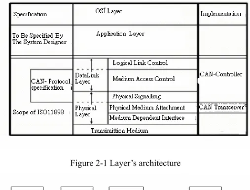
(14) 2.1 Introduction to CAN-BUS protocol. Figure 2-1 Layer’s architecture. Figure 2-2 CAN’s physical structure [10] CAN defines a physical layer and data link layers as shown in Figure 2-1 [9]. Physical layer includes the definition of transmission medium and logic level. In general, CAN network uses two signals named CANH and CANL to access the information, and the terminals should be two 120Ω resistors shown in Figure 2-2. Since it transmits data by two serial streams, the definition of logic level is different .It can be expressed as the binary values, 1/0. Binary ‘1’ is called recessive bit (CANH= CANL=2.5V) and binary ‘0’ is called dominant bit (CANH=3.5V; CANL=1.5V). Since the binary value is presented with the difference, bit level = (CANH+δ)-(CANL+δ), it has good capability of EMI noise rejection. Data link layers define the format, message filter, bit rate and arbitration. Here is some brief introduction of CAN’s characteristics. 4.

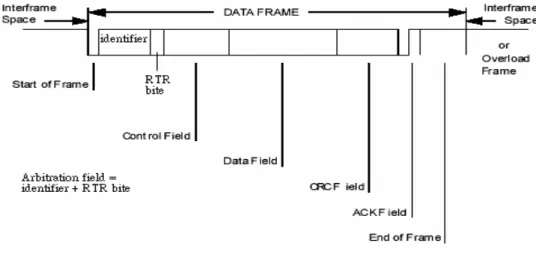
(15) Data frame:. Figure 2-3 Data frame format As shown in Figure 2-3, arbitration field includes CAN’s ID (ex. the steering angle sensor is 0C0) and RTR bit. Every message has an identifier, which is unique within the whole network since it defines content and also the priority of the message. The identifier with the lowest binary number has the highest priority. Arbitration: Whenever the bus is free, any node may start to transmit a message. If two or more nodes start transmitting messages at the same time, the bus access conflict is resolved by bit-wise arbitration using the identifier. The mechanism of arbitration guarantees that neither information nor time is lost. All nodes with lower priorities do not re-attempt transmission until the bus is available again. 2.2 8951 subsystem [9-11] In order to receive the CAN BUS signal and covert it to 16-bit data, 8951 system is composed of a transceiver (PCA82C251), a stand alone controller (SJA1000), and a 89C51. 2.2.1 Transceiver Transceiver is the interface between stand-alone controller and the physical layers of CAN network which converts CANH and CANL from physical layers to serial stream signals as the input of the stand–alone controller. So the host controller must access the data via the 5.

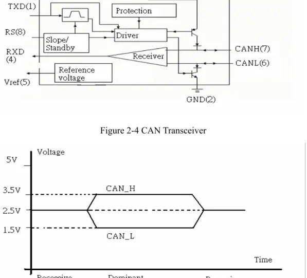
(16) transceiver. Figure 2-4 shows the transceiver’s pins and its internal blocks. The most important ones are CANH (Pin 7), CANL (Pin 6) and RXD (Pin 4). Because we use it only for receiving data, only these three pins should connect to the stand alone controller. The receiver’s comparator converts the differential bus signal to a logic level signal which is the output at RXD. The serial receive data stream is provided to the bus protocol controller for decoding. Figure 2-5 [9] shows the bus state: When CANH and CANL are both 2.5V, the bus is recessive (logic‘1’). When CANH is 3.5V and CANL is 1.5V respectively, the bus is dominant (logic‘0’).. Figure 2-4 CAN Transceiver. Figure 2-5 CAN BUS state 6.

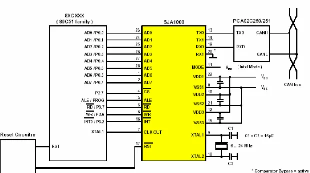
(17) 2.2.2 Stand-alone controller and 89C51. Figure 2-6 Block diagram of SJA1000 Figure 2-6 shows the block diagram of SJA1000 [10]. The CAN Core Block controls the transmission and reception of CAN frames according to the CAN. The Interface Management Logic block performs a link to the external host controller which can be a microcontroller or any other device. Every register access SJA1000 multiplexed address/data bus and controlling of the read/write strobes is handled in this unit. When receiving a message, the CAN Core Block converts the serial bit stream into parallel data for the Acceptance Filter. With this programmable filter, SJA1000 decides which messages actually are received by the host controller. All received messages accepted by the acceptance filter are stored within a Receive FIFO. Depending on the mode of operation and the data length up to 32 messages can be stored. Figure 2-7 shows the 8951 subsystem circuit [10]. Port 0 of 8951(address/data bus) is used to communicate with the stand alone controller SJA1000. We can set the register value in SJA1000 via this address/data bus. Since 8951 treats SJA1000 as the external memory, the address/data bus should cooperate with /RD and /WR signals. To set the register value, we should notice the mode of SJA1000 (reset mode or operation mode), this will be mentioned later.. 7.

(18) Figure 2-7 8951 subsystem Pin 11 of SJA1000: select the host controller family with Intel or Motorola mode. Intel mode: Mode=high Motorola mode: Mode=low The SJA1000 can operate with an on-chip oscillator or with external clock sources. Additionally CLK OUT (Pin 7) can be enabled to output the clock frequency for the host controller.. 2.2.3 Set the registers of SJA1000 When power on (SJA1000 is reset mode), we can set the registers: (a) Acceptance code. (b) Acceptance mask They can set the acceptance filter. The received data is compared bitwise with the value contained in the Acceptance Code register (ACR). The Acceptance Mask Register (AMR) defines the bit positions, which are relevant for the comparison (0 = relevant, 1 = not relevant). For accepting a message, all relevant received bits have to match the respective bits in ACR. In other words, if we set the AMR as “11111111”, all identifiers can be accepted.. 8.

(19) Figure 2-8 An example of acceptance filter Figure 2-8 explains how the acceptance filter works. The registers shown below are set in reset mode. (1) Bus-timing registers (2) Output control register (3) Command register When Pin 17 is low, SJA1000 enters operation mode. It starts receiving data and transmitting the 16-bit value to host controller. Figure 2-9 shows the flow diagram of data reception [10, 12]. The host controller reads the Status Register of the SJA1000 on a regular basis, checking if the Receive Buffer Status flag (RBS) indicates that at least one message has been received. The Receive Buffer Status flag indicates “empty” means no message has been received. The host controller continues with the current task until a new request for checking the Receive Buffer Status is generated. The Receive Buffer Status flag indicates “full” denotes one or more messages have been received.. Figure 2-9 Flow diagram of reception of a message [10,12]. 9.

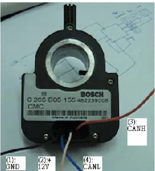
(20) Figure 2-10 Timing diagram of transmit data to controller Tx2 is a control signal generated by host controller. At its negative edge, host controller transmits high-8 bits steering angle data from Port 1. At its positive edge, host controller transmits low-8 bits steering angle data from Port 1.. 2.3 Steering angle sensor This sensor transmits signed 16-bit data (range:-7800~7800) and its identifier is 0C0 (hex), so the acceptance code of SJA1000 is 0C0 (“00001100000”). The sensor is Basic-CAN (CAN 2.0A) mode since it has 11-bit identifier. Table 2-1 Information of steering angle sensor Value in the message. Value in the message. (hex). (decimal). E188. -7800. Angle value in°. remark. -780°. Negative limit angle range. 1E78. 7800. 780°. Positive limit angle range. 7FFF. 32768. 3276.8°. 10. invalid.

(21) Figure 2-11 Steering angle sensor It is put around the steering wheel. When the steering wheel is turning, the sensor is also turning and measuring the steering angle. Figure 2-11 shows the steering angle sensor which mainly uses 4 pins: (1) GND, (2) +12V, (3) CANH, (4) CANL.. 2.4 Sketch of the yaw rate sensing system. Figure 2-12 Yaw rate sensor 11.

(22) Figure 2-12 shows the yaw rate sensor. The red wire is connected to +5V, the green wire is connected to GND and the white one is connected to output. It should be fixed to sense the yaw rate of the vehicle.. Figure 2-13 Peripheral circuits of yaw rate sensor. Figure 2-14 Comparison 12.

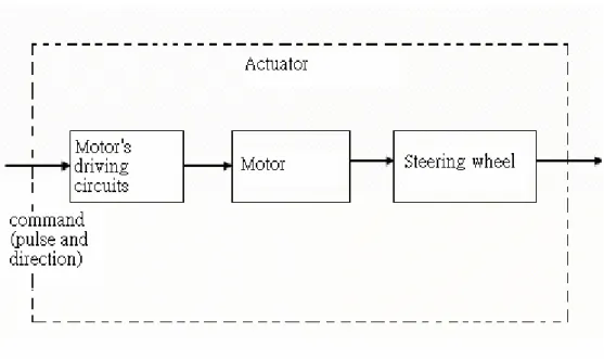
(23) Figure 2-13 shows yaw rate sensor peripheral circuits. Two OP amplifiers form a low pass filter. Since the signal from yaw rate sensor is easily disturbed by high frequency noises, the filter can reduce them. The output of low pass filter is treated as the input of ADC0804. Figure 2-14 shows the results with and without low pass filter. The upper signal is processed by low pass filter and the lower one is the original signal from yaw rate sensor. ADC0804 converts the analog sensor output to 8-bit digital input of FPGA, the pins /CS and /RD are tied at ground, and /WR control signal is fed by FPGA. At negative edge of /INTR, FPGA receives data from Pin 11 to Pin 18.. 2.5 Actuator Figure 2-15 is the block diagram of actuator which is composed of a motor, motor’s driving circuit and the steering wheel. This can implement the concept of steering by wire technique. The steering wheel is the load of motor, which is driven by the motor. Figure 2-16 shows the motor with its driving circuit and the steering wheel, there are several pins used for control. The most important is the switch which is directly operated by users so that the motor rotates if we press the switch.. Figure 2-15 Block diagrams of actuator 13.

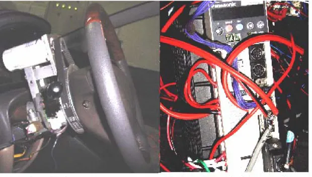
(24) Figure 2-16 The Actuator Our plant (motor) is associated with its driving circuit. In order to control the motor, we should transmit control signals to this driving circuit such as pulses. There are several methods to control the motor, the one we choose is to control rotation speed and rotation directions. Figure 2-17 shows the control signals of motor, which include the pulses and direction control signals. The higher frequency makes the steering wheel rotate faster. Sign 1 and sign 0 control the direction of rotation. But the frequency should be in the range of [0, 20khz]. High frequency may cause the motor damage.. Figure 2-17 Control signals of motor 14.

(25) Chapter 3 Design of Vehicle Lateral Control Systems Figure 3-1 describes the block diagram of proposed lateral control system. The FLC decides the desired steering angle. The inputs of FLC are error of yaw rate and the change of error. The output is treated as the command of the PD controller. It can not only reduce the difference between the actual steering angle and the desired one but also tune the speed of rotation. The desired yaw rate is predefined with the fixed path (ex: circle-path, s-path, etc.), at the low speed (ex: 20 km/h). The device “dSPACE” used to record the yaw rate.. Figure 3-1 The block diagram of proposed lateral control system 3.1 PD controller. Figure 3-2 PD controller 15.

(26) Figure 3-2 shows the PD controller [13], where kp is proportional gain and kd is derivative gain. As mentioned in Chapter 2, the direction and speed are two most important behaviors we should consider. First, we make the motor rotate in positive direction if the error is positive. (i.e. actual angle < desired angle ) and vise versa. Second, we make the motor rotate smoothly. In general, human rotates the steering wheel faster when the change of steering angle is larger. P control can implement this action. We must notice that the change of rotation speed should not be too large since the steering wheel will not rotate smoothly. In other words, D control produces little regulation to make the speed not too fast. When the error is positive, the regulation is negative. Otherwise, when the error is negative, the regulation is positive. It can improve the transient performance. For the whole system, the PD controller can be viewed as time delay since it just affects the yaw rate by means of controlling the steering wheel. And it ensures the steering angle is identical to the output of FLC.. 3.2 Introduction to FLC. Figure 3-3 Basic architecture of FLC 16.

(27) As shown in Figure 3-3, FLC is composed of four important parts [14]. (1) Fuzzifier: a fuzzifier performs the function of fuzzification which is a subjective valuation to transform measurement data into valuation of a subjective value. Hence, it can be defined as a mapping from an observed input space to labels of fuzzy sets in a specified input universe of discourse. Ex: NB (negative big); NM (negative medium); NS (negative small); ZE (zero) PB (positive big) ; PM (positive medium); PS (positive small). (2) Fuzzy rule base: fuzzy control rules are characterized by a collection of fuzzy IF-THEN rules in which the preconditions and consequents involve linguistic variables. The. general. form. of. fuzzy. control. rules. in. the. case. of. multi-input-single-output systems (MISO) is: Ri: IF x is A, AND y is B THEN z=C. (3.1). i =1,2,3,…,n where x, y and z are linguistic variables representing the process state variables and the control variables, respectively. A, B and C are the linguistic values of the linguistic variables x, y, and z in the universe of discourse U, V and W, respectively. (3) Inference engine: this is the kernel of the FLC in modeling human decision making within the conceptual framework of fuzzy logic and approximate reasoning. This is an example: IF x is A, THEN y is B. x is A1. Conclusion => y is B1. Fuzzy relation: AÆ B. 17.

(28) There are four operations usually used: a. Max-min operation. b. Max product operation. c. Max bounded product operation. d. Max drastic product operation. (4) Defuzzifier: it is a mapping from a space of fuzzy control actions defined over an output universe of discourse into a space of nonfuzzy (crisp) control actions. This process is necessary because in many practical applications crisp control actions is required to actuate the control. There is no systematic procedure for choosing a defuzzification strategy. Two common used methods of defuzzification are the center of area (COA) method and the mean of maximum (MOM) method.. ∑ µ (z )z ∑ µ (z ) n. ZCOA =. i =1 n. i =1. n. ZMOM =. c. i. c. i. i. zi. ∑n. (3.2). (3.3). i =1. 3.3 Fuzzification. Equations (3.4) and (3.5) are definitions of error and change of error for yaw rates. e (k)=r(k)-y(k). (3.4). ∆e(k ) = e(k) – e(k-1) ,. (3.5). where r (k ) is pre-defined yaw rate data, y (k ) is the actual data feedback via yaw rate sensor and e(k ) is the error. Because we get the feedback data via 8-bit A/D (ADC0804), the original yaw rate is in the range [0,255]. Where 0(“00000000”) represents -100°/s and 255(“11111111”) represents +100°/s. 18.

(29) Figure 3-4 Fuzzification. In our experiments, we don’t turn the steering wheel to extreme angles (i.e. too positive or too negative angles.) because we don’t drive the cars like this. So the error and change of error won’t be too large. (-100°/s~+100°/s) First, the inputs e(k) and ∆e(k ) must be normalized into the range [0,255] for convenience. If e(k) or ∆e(k ) is positive, it will be normalized into the range [128,255], and if e(k) or ∆e(k ) is negative, it will be normalized into the range [0,127]. Figure 3-4 is the diagram of fuzzification.. 3.4 Rule base. In Section 3.3, the inputs e(k) and ∆e(k ) both have 7 linguistic variables {NB, NM, NS, ZE, PS, PM, PB}. There are 49 rules. Let u(k) be output linguistic variable. Rule (1): IF e(k) is PB and ∆e(k ) is NB THEN u(k) is ZE. . Rule (25): IF e(k) is ZE and ∆e(k ) is ZE THEN u(k) is ZE. . . Rule (49): IF e(k) is NB and ∆e(k ) is PB THEN u(k) is ZE. These rules can be represented with a look-up table and listed in Table 3-1. 19.

(30) Table 3-1 Look-up table. 3.5 Inference engine. The method we use is singleton mechanism which is modified from max-min operation. Figure 3-5 shows singleton inference mechanism which is similar to max-min operation [15]. It is more convenient to store the centers of all triangles with lower membership values of min product so that it can reduce the complexity when defuzzyfing.. Figure 3-5 Singleton inference mechanism. 20.

(31) 3.6 Defuzzification. The output of fuzzy inference is a linguistic value. For control, we need to transfer it to a crisp value which is treated as a command of motor-steering wheel system. In our experiments, this crisp value must be mapped to the desired steering angle as shown in Figure 3-6. Use (3.2), we can derive the center of gravity so that the linguistic output of FLC can be obtained. In Section 3.5, we use singleton of inference mechanism to reduce the complexity in defuzzyfication. It is more convenient since the modified mechanism uses less point than max-min operation to calculate the crisp output. Also, it saves operation time when the implementation is done with FPGA.. Figure 3-6 Relationship between FLC output and motor-steering wheel desired angle. 21.

(32) Chapter 4 Implementation of Vehicle Lateral Control Systems FPGA (Field Programmable Gate Array) is the kernel of the system because of its speed of process and flexibility. We must write the functions with VHDL and then download them to the development board. If we will change the contents of the functions, we only re-write and download the new functions again after compiling. In Figure 4-1, ALTERA Stratix EP1S25 DSP development board is included with the DSP Development Kit, Stratix Edition. This board is a powerful development platform for digital signal processing designs, which features the Stratix EP1S25 device in the fastest speed grade 780-pin package. And we use Quartus4.0 as software for testing functions, downloading configurations to board and simulation.. Figure 4-1 Stratix development board. (EP1S25F780) 22.

(33) In FPGA, logic ‘1’ is 3.3V and logic ‘0’ is 0V. When connecting the I/O pins to external circuit (ex. 8951), we must adhere to the voltage restrictions. Specifically, the I/O pins are not 5V tolerant and should not be directly connected to logic powered from a 5V supply.. 4.1 8951 subsystem. Besides CAN stand-alone controller (SJA1000), transceiver (PCA82C250) and the steering angle sensor, it is important that 8951 communicates with FPGA. It is impossible to decode the data or control the vehicle without communication. Hence, Port 1 (Port 0, and some pins such as /WR, /RD, are used for communication with CAN stand-alone controller) and some other pins of 8951 are used for communication with FPGA, the role they play is transmitting control signals and sensing data.. Figure 4-2 Communication with FPGA 23.

(34) As shown in Figure 4-2, 8951 communicates to FPGA with 10 pins. (Port 1, P3.1, P3.5 ) Port 1 is treated as data bus which is controlled by control signal tx2. It must transmit 8-bit data twice since the sensing data is 16-bit. The high 8-bit data is transmitted when tx2 is at negative edge and the low 8-bit data is transmitted when tx2 is at positive edge. Finally, another control signal “start” requests FPGA to convert the original 16-bit data to signed decimal angle value when it is at positive edge. Figure 4-3 shows these control signals and their waveforms. The upper one is “start” and the other is “tx2”. It is important that “start” signal activates after 8951 finishes transmitting data (i.e. FPGA finishes receiving data). In other words, “start” enables when “tx2” is high in order to avoid transmitting transient values. It takes about 3.5ms to transmit 16-bit data and FPGA converts the data every 7ms.. Figure 4-3 Control signals. 24.

(35) Figure 4-4 Block diagram for converting angle value Figure 4-4 shows the block diagram of FPGA for decoding sensing data of steering angle. FPGA stores the 16-bit data after receiving 8-bit data twice and converting it to signed decimal value. Finally, FPGA shows the results with three 7-segment LEDs. Another LED shows the sign of data, it illuminates when the value is negative.. 4.2 Communication with yaw rate sensor. As mentioned in Chapter 2, FPGA should obtain yaw rate data through A/D (ADC0804) , the reason is not only receiving data but also transmitting control signal to ADC0804’s /WR pin. As the result, ADC0804’s pin /INTR transmits signal to FPGA. ADC0804 finishes converting analog data to digital data when /INTR=’0’. So we set FPGA to receive data from yaw rate sensor at /INTR’s negative edge. It is important that the frequency of /WR must be less than 10MHZ. Figure 4-5 shows the relationship between /INTR and /WR. For the purpose of control, we let ADC0804 transmit data every 0.13s.. 25.

(36) Figure 4-5 /WR and /INTR After receiving sensing data from yaw rate sensor, FPGA determines the degree of yaw rate and shows the result in several LEDs which illuminate when yaw rate reaches some values such as +10° or -10° ,etc. At the same time, FPGA calculates the error of yaw rate and the change of error which will be treated as the inputs of FLC.. 4.3 Implementation of PD controller [16, 17]. This controller is used for controlling the motor which drives our steering wheel. It controls not only the directions but also the speed of rotation. Figure 4-6 shows the block diagram of FPGA for implementation of a PD controller. The most important part is “control block” which contains several control signals playing important roles. PD parameters, kp and kd, are labeled pgain and dgain, respectively.. 26.

(37) Figure 4-6 Block diagram of a PD controller in FPGA. Figure 4-7 Timing diagram of control block 27.

(38) As Figure 4-6 shows, the reference angle is the stream “target” which comes from FLC or from user when testing. The stream “ch” is feedback data through steering angle sensor. The stream cerr1 is the difference with previous error and new error. The control block generates signals tem1, sub1, load1 and mul1 with input signals of clk and start from 8951.When signal “start” activates, the PD controller gets reference input and actual angle output in order to calculate error and change of error. The register nxt loads err1 at tem1’s positive edge; the register cer1 loads nxt-pre (change of error) at sub1’s positive edge; the register pre loads last nxt at load1’s positive edge. Finally, when mul1 is at positive edge, the multiplier enables so that it uses pgain and dgain to obtain pd as (4.1). pd= ( pgain*err1) + ( dgain*cerr1).. (4.1). where pgain is kp of the PD controller, dgain is kd of the PD controller, err1 is the error of rotation angle and cerr1 is the change of error. The first bit of the stream pd (it has 17 bits) indicates the sign of direction and the others indicate the absolute values of speed. Table 4-1 Directions of rotation pd(16)=’0’. (positive). Left (direction of rotation). pd(16)=’1’. (negative). Right (direction of rotation ). As Table 4-1 shows, the steering wheel will turn left if the sign (the first) bit is’0’ and turn right if it is ‘1’. Table 4-2 indicates the relationship between speed and the absolute value of the stream pd. The output frequency becomes large when the absolute value of pd in (4.1) is increased but the output frequency is zero when the absolute value of pd is very small. At this time, the motor doesn’t rotate and the steering angle holds at fixed value. Since the range of frequency (motor’s input) is less than 20KHZ, we set the frequency less than 19.53KHZ. The frequency is determined by division factor, which depends on the range of the absolute value of pd. And the base frequency is 39.06KHZ generated in FPGA.. 28.

(39) Table 4-2 Speed of rotation pd(15 downto 0). Division factor. Output frequency (speed). >800. 2. 19.53KHZ. 600~800. 4. 9.77KHZ. 400~600. 6. 6.51KHZ. 200~400. 8. 3.91KHZ. 100~200. 12. 3.26KHZ. 40~100. 20. 1.95KHZ. 10~40. 26. 1.5KHZ. 0~10. --. 0. For example, if sign bit of pd is ‘1’ and the absolute value of pd is 500, then the direction is right and division factor is 6, the output frequency (input of driver) is 39.06 / 6 = 6.51 KHZ.. 4.4 Implementation of FLC [16, 17]. The basic architecture of the FLC contains fuzzifier unit, inference unit, deffuzifier unit and control unit. The specifications of proposed FLC are listed below: (1) 2 inputs (error of yaw rate, change of error.) and 1 output. (2) Universe of discourse is 8-bit (0~255). (3) Membership values are 3-bit (0~7). (4) Each universe of discourse is divided into seven subsets: NB (negative big), NM (negative medium), NS (negative small), ZE (zero), PS (positive small), PM (positive medium), and PB (positive big).. 29.

(40) (5) Overlapping = 2. (6) There are 49 fuzzy rules. (7) The membership functions are stored in ROM.. 4.4.1 Design of fuzzifier unit. The main work of fuzzifier unit is converting the crisp input values to corresponding membership functions and determining activation rules, their membership values and the center of output membership functions. We use two ROMs to store these data, the crisp input value are directly treated as the address of ROMs so that it is convenient to accomplish fuzzification. Figure 4-8 illustrates how the fuzzifier unit stores the input vales as fuzzy set. As mentioned in Chapter 3, the two inputs e and ce are normalized to the range [0,255] (8-bit), and there are 7 membership functions and the overlapping =2. The input membership functions are divided into 6 orders (000~101) in according to the overlapping. And each order has two parts: high and low (low has non-increasing slopes and high has non-decreasing slopes in each order), which represent the membership values belong to two adjacent membership functions. Tables 4-3 to 4-5 illustrate how the above data will be stored.. 30.

(41) Figure 4-8 Input membership functions. Table 4-3 Storage of inputs e and ce (order) Order. 000. 001. 010. 011. 100. 101. Address(input). 0~101. 102~114. 115~126. 127~139. 140~151. 152~255. Table 4-4 Storage of inputs e and ce (low) Stored data(low) Address (input) Address (input) Address (input) Address (input) Address (input) Address (input). 111. 110. 101. 100. 011. 010. 001. 000. 0~70. 71~74. 75~78. 79~82. 83~87. 88~92. 93~97. 102~ 103 115~ 116 127~ 128 140~ 141 152~ 154. 104~ 105 117~ 118 129~ 130 142~ 143 155~ 159. 106~ 107 119~ 120 131~ 132 144~ 145 160~ 164. 108~ 109 121~ 22 133~ 134 146. 110. 111~ 112 124~ 125 136~ 137 149. 113~ 114 126. 98~ 101 --. 165~ 168. 31. 123 135 147~ 148 169~ 172. 173~ 176. 138~ 139 150~ 151 177~ 181. ---182~ 255.

(42) Table 4-5 Storage of input e and ce (high) Stored data (high) Address (input) Address (input) Address (input) Address (input) Address (input) Address (input). 000. 001. 010. 011. 100. 101. 110. 111. 0~70. 71~74. 75~78. 79~82. 83~87. 88~92. 93~97. 98~101. 102~ 103 115~ 116 127~ 128 140~ 141. 104~ 105 117~ 118 129~ 130 142~ 143. 106~ 107 119~ 120 131~ 132 144~ 145. 108~ 109 121~ 122 133~ 134. 111~ 112 124~ 125 136~ 137. 113~ 114. 146. 147~ 148. 149. 155~ 159. 160~ 164. 165~ 168. 169~ 172. 173~ 176. 177~ 181. ----152~ 154. 110 123 135. 126 138~ 139 150~ 151 182~ 255. Notice that high and low only have the values “000” or “111” when the order is “000” or “101”, because in these orders, the values are more positive or negative than those in the other orders, the weight (high or low) can take extreme values (“000”). Figures 4-9 and 4-10 indicate the block diagrams of fuzzification units for two inputs, e and ce , respectively. Each fuzzification unit is composed of multiplexers, ROMs, and control units.. Figure 4-9 Fuzzification unit for input e. 32.

(43) Figure 4-10 Fuzzification unit for input ce The control unit generates a control signal for each multiplexer and it selects e or ce as the address bus of ROM. At the same time, control unit sends a trigger signal to ROM for reading data. The data read from ROM consists of “order”, “high” and “low”. “Order” generates “order_1” with an increment circuit. Hence, “order” and “order_1” represent the activated membership functions. And the two values, “high” and “low” represent membership values in “order” and “order_1”, respectively. These data are prepared for inference.. 4.4.2 Design of inference unit. Table 4-6 illustrates the output gravities (8-bit). The first 3 bits of address come from order1 or order1_1 and the others come from order2 or order2_1. It is output gravities that the inference unit only stores since we use the method of singleton mechanism. And each gravity value needs 8 bits for storage, so it takes 49*8=392 bits of ROM for these data.. 33.

(44) Table 4-6 Gravities of inference Gravity. 00000010 00000111. 00001100. 00010010 00011000. 00011110. 00100100. 000101. 000110. Address 000000. 000001. 000010. 000011. 000100. Gravity. 00110000. 00110110. 00111100. 01000010 01001000 01010001. Address 001000. 001001. 001010. 001011. 001100. 001101. 001110. Gravity. 01100001. 01101001. 01101111. 01110101. 01110111. 01111001. Address 010000. 010001. 010010. 010011. 010100. 010101. 010110. Gravity. 01111101. 01111111. 10000000 10000001 10000010 10000100. Address 011000. 011001. 011010. 011011. Gravity. 00011010. 01011010. 01111011. 10000110. Address 100000 Gravity. 011101. 011110. 10001000 10001010 10010000 10010110. 10011100. 10100010. 100001. 10101001 10110000. 011100. 100010. 100011. 100100. 100101. 100110. 10111000. 11000011. 11001001. 11001111. 11010101. Address 101000. 101001. 101010. 101011. 101100. 101101. 101110. Gravity. 11100001. 11100111. 11101100. 11110010. 11111000. 11111101. 110001. 110010. 110011. 110100. 110101. 110110. 11011100. Address 110000. Figure 4-11 Inference unit 34.

(45) Inference unit is shown in Figure 4-11. The inputs of the multiplexers are order1, order1_1, order2, and order2_1 (all of them are 3-bit) which generates four addresses since the controller is two inputs and overlapping =2 (a maximum of 4 rules can be activated at any time.). The gravities will be stored in ROM and the output gravity (gi) will be send to defuzzifier unit. At the same time, the other multiplexer selects corresponding “low” and “high” value. The next step is to find the minimum membership (or fire strength, fi.) between the two antecedents of each active rule and the rule consequent. The minimum circuit compares the antecedents of each active rule and outputs the minimum membership value whereas linguistic labels of the antecedents address the position in the rule memory storing the corresponding consequent for each rule. A ROM enable signal, clk_2, from the control unit, enables the ROM. The selections of multiplexers are controlled by the 2-bit signal (s1 and s0) as shown in Table 4-7. Table 4-7 The combinations of inference output S1. S0. Address. MIN. 0. 0. order1&order2. low1 & low2. 0. 1. order1&order2_1. low1 & high2. 1. 0. order1_1&order2. high1 & low2. 1. 1. order1_1&order2-1 high1 & high2. 4.4.3 Design of defuzzification unit. Defuzzification unit processes the outputs of inference unit, output gravities and fire strength in order to generate a crisp output value u (command). There are at most 4 active rules since the system has two inputs and one output. And the method for defuzzification is “center of gravity” which is derived from center of area (COA) and singleton inference mechanism since the output of inference is gravity instead of area. 35.

(46) 4. u=. ∑f. i. * gi. i=1. (4.2). 4. ∑f. i. i=1. Figure 4-12 is the block diagram of fuzzy mean module for defuzzification. The inputs, gi (output gravity) and fi (fire strength) are both from inference unit. This module uses an accumulator which accumulates the numerator by adding the new product with the previous product. Another accumulator adds the fire strength of antecedents with the new fire strength as the denominator of (4.2). Each accumulator is composed of an adder and a register, and the signal “ld” controls the actions of accumulation. After accumulating four times, another signal “div” enables the divider to operate with its inputs, numerator and denominator. Finally, we can get the crisp output value u.. Figure 4-12 Defuzzification unit. 36.

(47) 4.4.4 Design of control unit. This unit is a sequential circuit which generates control signals. Figure 4-13 is the timing diagram of these signals producted by Quartus4.0 software. The inputs are clock signal (clk) and reset signal (rst); the outputs are control signals such as clk_1, clk_2, ld, div, and s.. Figure 4-13 Simulation of control unit 4.4.5 Lookup table for fuzzy output. In order to transform the output of FLC to reference angle for controlling steering wheel, we use a lookup table. The yaw rate becomes “positive large” when the steering wheel is turned right, but the steering angle becomes “negative large” at the same time. Hence, the sign of these sensors are different so that it is necessary to build a lookup table to overcome this problem. As Table 4-8 shows, we have a “dead-zone” when u is in the range of [123, 133]. In this region, modification angle is zero to avoid oscillation of steering wheel. In other words, the steering wheel is out of action at this time. Besides dead-zone, the modification of steering angle is negative when the output of FLC u is larger than 134 (it means that we should turn right). And the “value” of modification becomes larger when u leaves dead-zone more. In other words, like driven by a human, vehicle needs more “strength” to desired behavior when the offset is larger. For example, modification is -50° when u is 135. And there is a restriction to modification angle: the value should be less than 120° to 37.

(48) avoid the reference angle getting more than the extreme value of steering wheel. The reference angle of steering wheel is controlled by the modification. Like the accumulator of defuzzifier, another accumulator controlled by another control signal “an” adds previous reference angles with new signed modification angle as new ones. Figure 4-14 and (4.3) can explain how this accumulator works.. θ (k ) = θ (k − 1) + ∆θ (k ). (4.3). In (4.3), θ (k ) is the new reference angle, θ (k − 1) is the previous reference angle, and. ∆θ (k ) is modification angle. Table 4-8 Lookup table for u and modification angle Fuzzy output u. Modification angle (to steering wheel). >177. -120°. 134~177. -2.5° * (u-133). 123~133. 0°. 78~122. 2.5° * (123-u). <77. 120°. Figure 4-14 Block diagram for modification and reference steering angles. 38.

(49) Chapter 5 Experimental Results The experiments are divided into two parts: static part and dynamic part .The former tests steering wheel including CAN BUS decoding system (8951 subsystem), motor driving, and a PD controller. The latter includes not only static part but yaw rate system and a FLC. Hence, dynamic experiments show real vehicle behaviors with low speed (about 20km/h.).. 5.1 Experimental platform. As mentioned in Chapters 2 and 4, we use two sensors to obtain the data of the steering angle and the yaw rate. The platform of our experiment includes 8951 subsystem (Peripheral circuit is shown in Figure 5-1.) for receiving CAN BUS data, FPGA for control and signal process, a motor and its driving circuit as the actuator, dSPACE in Figure 5-2 for recording data, and the experimental car, TAIWAN iTS-1 (Figure 5-3.) for experiment.. Figure 5-1 Peripheral circuit. 39.

(50) Figure 5-2 dSPACE for recording data. Figure 5-3 Experimental car, TAIWAN iTS-1 5-2 Results of rotating the steering wheel to reference angle Case 1: Test of the angle (+80°). Figure 5-4 (a) is the reference of the steering angle, the command is like a step function with “height” of +80°. Figure 5-4 (b) is the response of steering angle, notice that the steering wheel can reach desired angle (+80°) within 1s and the PD controller can modulate the speed of rotation. The oscillation after 1.5s is relatively small so that it won’t affect the behavior of vehicle (rotational angle of the front tires). 40.

(51) Steering angle (degree). Time (sec) Figure 5-4 (a) Reference angle (+80°) Steering angle (degree). Time (sec) Figure 5-4 (b) Response of the steering angle. 41.

(52) Case 2: Test of bidirectional reference angles (±80°). Steering angle (degree). Time (sec) Figure 5-5 (a) Reference angle of ±80° Steering angle (degree). Time (sec) Figure 5-5 (b) Response of the steering angle As Figure 5-5 (a) shows, the command is composed of several step functions, and the reference angles are +80°, -80°, and 0°. Figure 5-5 (b) is the response of steering angle. The steering wheel rotates to desired angles. 42.

(53) and then locked by the controller at those angles. Case 3: Test of bidirectional reference angles (±200°). Steering angle (degree). Time (sec) Figure 5-6 (a) Reference angle of ±80° Steering angle (degree). Time (sec) Figure 5-6 (b) Response of the steering angle In order to prepare for “dynamic” experiments that control yaw rate of the car, it is necessary to test the bidirectional reference angles of ±200°. 43.

(54) Figure 5-6 (a) is the reference angles including +200° (t=1s) and -200° (t=5s). Figure 5-6 (b) shows the result. Obviously, the delay time is longer if the difference between actual angles and reference ones is larger. 5-3 Results of controlling the yaw rate. After examining the steering wheel and ensuring that it can be controlled at desired angles, we need to test the behavior of our experimental car. Yaw rate is the dynamic property we emphasis on. Hence, the response of yaw rate will be represented later. However, yaw rate not only depends on steering angle but also speed, so we will consider the effects of speed and steering angles. Case 1: Lower speed (Turn right). The steering angle is negative and the yaw rate is positive when we turn right. Figures 5-7(a), 5-7(b) and 5-7(c) verifies that both speed and the steering angle affect the yaw rate. At lower speed (Figure 5-7 (a),about 5km/h ~ 11km/h), the reference yaw rate is about 14°/s (Figure 5-7 (c)), but the steering angle reaches the extreme value (Fgure 5-7 (b),-420°) to maintain the reference yaw rate. In Figure 5-7 (c), the output is close to 14°/s, it means that the lateral control system controls the yaw rate as we wish. Although there is error caused by DC offset of the sensor, the controller can modulate them to the reference values.. 44.

(55) Speed (km/h). Time (sec) Figure 5-7 (a) Speed Steering angle (degree). Time (sec) Figure 5-7 (b) Steering angle 45.

(56) Yaw rate (°/s). Time (sec) Figure 5-7 (c) Yaw rate Case 2: At about 18km/h (Turn right). In Figure 5-8 (a), we will drive the experimental car at the speed about 18km/h. The steering angle shown in Figure 5-8 (b) will no longer need to rotate to extreme value for vehicle to reach the reference yaw rate (20°/s.). Figures 5-8(a), 5-8(b) and 5-8(c) verifies that both speed and the steering angles affect the yaw rate again. The controller can modulate the error of the yaw rate by modifying the steering angles. In experiments, the steering wheel modulated the angle and the rotational speed like driven by human, and the experimental car moved in a circle as expected.. 46.

(57) Speed (km/h). Time (sec) Figure 5-8 (a) Speed Steering angle (degree). Time (sec) Figure 5-8 (b) Steering angle. 47.

(58) Yaw rate (°/s). Time (sec) Figure 5-8 (c) Yaw rate Case 3: At about 18km/h (Turn left). Similar to Case 2, this case tests for turn to left and the reference yaw rate is -20°/s. Results are shown in Figures 5-9(a), 5-9(b) and 5-9(c). With the stable speed, the steering angle had a little change to maintain the steady value of yaw rate. This verifies that the controller can handle well regardless of turning right or left at low speed.. 48.

(59) Speed (km/h). Time (sec) Figure 5-9 (a) Speed Steering angle (degree). Time (sec) Figure 5-9 (b) Steering angle 49.

(60) Yaw rate (°/s). Time (sec) Figure 5-9 (c) Yaw rate 5-4 Required resource of hardware Table 5-1 indicates the resource of hardware (FPGA) used for this system. We use about. 7% LE (logic element), 124 pins and 1024 bits of memory (less than 1% of total memory) to implement the lateral control system. Table 5-1 Required resource of FPGA Total logic elements. 1780/25660(7%). Total pins. 124/598 (21%). Total memory bits. 1024/1944576(<1%). 50.

(61) Chapter 6 Conclusions and Future Researches In this work, we have developed a FPGA based fuzzy and lateral control method to design a steering controller which mainly regulates yaw rates to reference ones by means of controlling steering angles. This is antecedent to the work of lane change. Besides, we have accomplished a 8951 subsystem to receive and decode the data from the CAN-BUS based steering angle sensor The speed is as important as steering angles to control yaw rates. With the same reference yaw rates, the steering angle is larger if we drive the car at lower speed. And the reference yaw rates are user-defined. In future researches, the speed may be an input of the controller, and another input should be added is the vision information, this can replace the reference yaw rates because we could design a controller to decide the reference yaw rates instead of user-defined ones in according to the vision based input. To insure safety and avoid damage of devices such as steering wheel, there are some restrictions. For example, the modification angle of steering wheel should not be too large since this may change the yaw rate a lot in a short period of time and may cause discomfort. Hence, in future work, not only performance but also safety and comfort need to be considered.. 51.

(62) Reference [1] N. Matsumoto, H. Kuraoka, and M. Ohba, “An experimental study on vehicle lateral and yaw motion control,” Proceedings of Industrial Electronic, Control and Instrumentation International Conference, vol.1, pp.113-118, 1991.. [2] M. Fu, J. Ruan, and Y. Li, “A new kind of robust design method of intelligent vehicle lateral control,” Intelligent Control and Automation, WCICA Fifth World Congress, vol.3, pp.2438-2442, 2004. [3] M. Hosaka and T .Murakami, “Yaw rate control of electric vehicle using steer-by-wire system,” Advanced Motion Control, The 8th IEEE International Workshop, pp.31-34, 2004. [4] T. Hessburg and M. Tomizuka, “Fuzzy logic control for lateral vehicle guidance,” IEEE Control Systems Magazine, vol.14, pp.55-63, 1994.. [5] Q. Zhou and F. Wang, “Driver assisted fuzzy control of yaw dynamics for 4WD vehicles,” Proceedings of 2004 IEEE Intelligent Vehicles Symposium, pp.425-430, 2004.. [6] J. Huang, J. Ahmed, A. Kojic, and J.-P Hathout, “control oriented modeling for enhanced yaw stability and vehicle steerability,” Proceedings of American Control Conference, vol.4, pp.3405-3410, 2004. [7] S. Mammar, Sainte-Marie, and S. Glaser, “On the use of steer-by-wire systems in lateral driving assistance applications,” IEEE Robot and Human Interactive Communication, International Workshop, pp.487-492, 2001.. [8] 吳政育, 林海平, “智慧型車輛之線控轉向模擬”, 大葉大學車輛工程學系碩士論文, 民國 92 年. [9] Motorola, Bosch Controller Area Network (CAN) Version2.0 protocol standard. [10] Philips Semiconductors, SJA1000 stand-alone CAN controller application note. [11] Philips Semiconductors, PCA82C250/251 CAN Transceiver Application note.. 52.