具Quanto特性的鎖高型權益連動年金之評價 - 政大學術集成

全文

(1)國立政治大學金融系所博士論文. 指導教授：陳松男博士. 治政大Annuities with Pricing Ratchet Equity-Indexed 立 ‧ 國. 學. Quanto Features. 具 Quanto 特性的鎖高型權益連動年金之評價. ‧. n. er. io. sit. y. Nat. al. Ch. engchi. i n U. 研究生：邱于芬民國九十九年九月 1. v.

(2) 謝辭. 在這段不算短的博士班生涯中，感謝一路上有體恤我的師長以及支持我的家人，讓我得以順利的取得博士學位。首先，我要感謝的是恩師陳松男教授。陳教授是位治學嚴謹的學者，平時除了專業知識的傳授之外，更常常不厭其煩的與我們分享. 政治大. 他的人生經驗以及學術研究的心得。每每在進度延宕、心情低落時，. 立. 老師的一番鼓勵總能令我有如醍醐灌頂般豁然開朗。感謝老師在論文. ‧ 國. 學. 的方向上給我相當多的想法以及建議，並於轉任上海高級金融學院之. ‧. 後仍費心幫我安排口試相關事宜。師恩浩瀚，永銘於心。. Nat. io. sit. y. 另外，要感謝口試委員彭火樹教授、江彌修教授、鄭士卿教授以. er. 及吳庭斌教授在口試時所提供的寶貴意見，讓我的論文更趨完整。. al. n. v i n Ch 感謝我的父母總在我最需要的時候，適時的伸出援手，無怨無悔 engchi U. 的陪我走過人生的每個階段。摯愛的老公一直是我精神上以及經濟上的最大支柱，謝謝你。最後，謝謝三個親愛的小寶貝，你們是我最大的成就，也是我繼續往前的最大動力。. 2.

(3) 摘要 Quanto EIA 是一種具有選擇權特性且能連結至外幣投資的保險年金商品。以往針對權益連動年金所做的文獻中，均未考慮 Quanto 的特性。本文利用風險中立評價法求算出六種具有 Quanto 特性的鎖高型權益連動年金商品的評價公式，並進一步利用數值分析來探討各個契約及市場參數對契約價值的影響。. 立. 政治大. ‧. ‧ 國. 學. 關鍵字：權益連動年金，外匯，風險中立評價法. n. er. io. sit. y. Nat. al. Ch. engchi. 3. i n U. v.

(4) Abstract Quanto Ratchet EIAs link to foreign investments and provide options-like properties. The literature covers the pricing of the EIAs that are not quantos. to fill the hole.. This paper intends. To derive the pricing formulas, we added an exchange rate model as. well as a foreign risk-free rate model to the pricing framework of Black and Scholes. Our formulas cover quanto ratchet EIA products for both compound and simple. 政治大. versions that may have a return cap and employ two types of geometric return. 立. averaging. We further provide numerical analyses on how contract features and. ‧ 國. 學. market parameters affect the contract value.. ‧. n. al. er. io. sit. y. Nat. Keywords: Equity-indexed annuities, foreign exchange, risk-neutral valuation.. Ch. engchi. 4. i n U. v.

(5) Contents 1.. INTRODUCTION ............................................................................................................ 7. 2.. PRODUCT SPECIFICATION AND VALUATION ..................................................... 10 2.1 Product Specification..................................................................................................... 10 2.2 Risk-Neutral Valuation.................................................................................................. 12. 3.. PRICING FORMULAS.................................................................................................. 15 3.1 Quanto Ratchet EIAs without Index Averaging ............................................................ 15. 3.1.1 Simple Quanto Ratchet EIAs ...................................................................... 15 3.1.2 Compound Quanto Ratchet EIAs................................................................ 17. 政治大 3.3 Quanto Ratchet EIAs with G2 Index Averaging ........................................................... 19 立. 3.2 Quanto Ratchet EIAs with G1 Index Averaging ........................................................... 17. NUMERICAL ILLUSTRATIONS................................................................................. 22. 學. ‧ 國. 4.. 4.1 Valuation Examples....................................................................................................... 22. Impact of return cap ............................................................................. 23. 4.2.2. Impact of Return Floor Rate ................................................................ 25. 4.2.3. Impact of Participation Rate ................................................................ 26. 4.2.4. Impact of Return Averaging ................................................................. 27. y. sit. er. io. al. v i n C h of Linked IndexU.............................................. 28 Impact of the Volatility engchi n. 4.2.6. Nat. 4.2.1. 4.2.5. 5.. ‧. 4.2 Parameter Analyses ....................................................................................................... 22. Impact of the Volatility of Exchange Rate ........................................... 29. 4.2.7. Impact of the correlation coefficient of log(S(t)) and log(C(t)) ........... 30. 4.2.8. Impact of the Domestic Risk-Free Rate ............................................... 31. 4.2.9. Impact of the Foreign Risk-Free Rate .................................................. 32. CONCLUSIONS ............................................................................................................ 33. References ............................................................................................................................... 37. 5.

(6) Table of Figures. Figure 1: Impact of Return Cap c ................................................................................ 24 Figure 2: Impact of return floor rate f .......................................................................... 25 Figure 3: The impact of Participation rate ................................................................... 27 Figure 4: Impact of Return Averaging ......................................................................... 28 Figure 5: Impact of the volatility of the linked index .................................................. 29. 政治大 Figure 6: Impact of the volatility of exchange rate ...................................................... 30 立. ‧ 國. 學. Figure 7: Impact of the correlation coefficient of log(S(t)) and log(C(t)) ................... 31. ‧. Figure 8: Impact of the domestic risk free rate ............................................................ 32. n. al. er. io. sit. y. Nat. Figure 9: Impact of the foreign risk free rate ............................................................... 33. Ch. engchi. 6. i n U. v.

(7) 1. INTRODUCTION. Since the recent turmoil in financial markets, products that eliminate the downside risk while still providing upside potential are in great demand.. Equity-indexed. annuities (EIAs) are such products. An EIA is a hybrid between a variable and a fixed annuity that allows the policyholder to participate in the potential appreciation of the stock market while eliminating the downside risk by a minimum return guarantee.. 政治大 The sales in 2008 is $26 billion, a 6% increase over 2007, and the sales 立. ‧ 國. 學. in 2009 is $30.1 billion, a 15.4% increase over 2008. 1. ‧. The product designs of EIAs are diverse, but can be divided into three major. sit. n. al. er. The return of the point-to-point EIA is determined by the. io. Asian-end designs).. y. Nat. categories: point-to-point, ratchet, and look-back (including the high-water-mark and. Ch. i n U. realized return of the linked index between two time points.. engchi. v Ratchet EIAs are more. favorable because returns are credited periodically with a guaranteed minimum and the account value never decreases once the return is credited.. A popular design of. the look-back EIA is the high-water-mark that earns the highest return on the index attained during the life of the contract. Among the three categories, ratchet EIAs are the most popular in the markets. Ratchet EIAs may vary in contract features such as reset frequency, return 1. Please see online reports on Advantage Compendium (http://www.indexannuity.org) 7.

(8) accumulation, return cap, and return averaging.. Most ratchet EIAs have the. annual-reset feature meaning that the return is credited to the contract annually. annual return may be accumulated in two ways.. The. The simple version of ratchet EIAs. add the annual returns up to give the final payout while the returns in the compound version are accumulated compoundedly.. To reduce the costs of EIAs, the insurer. may place a fixed upper limit, also called ceiling or cap, on the annual return.. It may. 政治大. also employ an averaging scheme in calculating the annual return to reduce the. 立. volatility of credited returns and thus the costs of guarantees.. For instance, an. ‧ 國. 學. insurer may calculate the geometric average of the index return over several. ‧. sub-periods as the credited return of the period.. Nat. io. sit. y. The pricing and hedging of EIAs have been studied by several researchers, and. er. many of them adopted the Black-Scholes assumptions (Black and Scholes, 1973).. al. n. v i n C solutions Tiong (2000) derived closed-form U major product designs by h e n gforcthe h ithree means of Esscher transforms.. Gerber and Shiu (2003) provided closed-form. formulas for lookback options and dynamic guarantees embedded in EIAs.. Lee. (2003) proposed four designs of EIAs to increase participation rates and derived the associated pricing formulas. ratchet EIAs.. Hardy (2004) presented a lattice method for valuing. Extending the Black-Scholes assumption of constant risk-free rate to. stochastic interest rates, Lin and Tan (2003) determined the fair participation rates for 8.

(9) the three major designs of EIAs numerically under Vasicek (1977) short rate model. Jaimungal (2004) assumed that the underlying index followed a geometric Variance-Gamma process and developed closed-form expressions for prices of point-to-point and ratchet EIAs.. Recently, Kijima and Wang (2007) adopted the. extended Vasicek model and derived the explicit pricing formulas for ratchet EIAs. Our contribution to the literature in this dissertation is that we derive the. 政治大 A contract is a quanto or. pricing formulas for ratchet EIAs with the quanto feature.. 立. cross-currency if the linked index is dominated in a different currency (e.g., Baxter. ‧ 國. 學. and Rennie, 1996; Hull, 2006). For instance, the contracts pay off in Australian. ‧. dollar and the linked index is S&P 500 which is dominated in US dollar.. Many variable (also called unit-linked). io. sit. y. Nat. feature is common in the derivatives market.. The quanto. Target customers. er. products of life insurance and annuities also have this feature.. al. n. v i n include the people interested in C international for their portfolios and h e n gdiversification chi U the people who live in the countries with less-developed capital markets and want to invest in more-developed markets.. Quanto ratchet EIAs are particularly popular in. areas such as Asia and Australia.. To incorporate the quanto feature, we add an. exchange rate model to the pricing framework.. The results of this dissertation are. mainly closed-form solutions for various ratchet EIA products with the quanto feature.. 9.

(10) 2. PRODUCT SPECIFICATION AND VALUATION. 2.1 Product Specification The fundamental variable in pricing ratchet EIAs is the annual return calculated based on the linked index.. Let T be the maturity of an EIA contract and S(t) be the linked. index at t ≤ T . Then the annual return of the linked index over the tth year will be: Rt =. 立. S (t ) , 治 t = 1,2, T . 政 S (t − 1) 大. (1). Insurers often take averages of the index returns over sub-periods of a year. ‧ 國. 學. when calculating the annual return to reduce the guarantee costs through dampening We analyze two types of geometric averaging in. y. Nat. io. sit. In the first case (which we refer as G1 hereafter), the annual return. er. this dissertation.. ‧. the volatility of credited returns.. over the tth year, Rt ,G1 , is taken as the geometric average of index sampled at an. n. al. interval of 1/m.. That is,. Ch. engchi. i n U. v. 1. i +1  m  S t ( − 1 + ) m 1 −  m  . Rt ,G1 = ∏   i =0 S (t − 1 + i )  m   For the second case (referred as G2 hereafter), the annual return over the tth year is denoted by Rt ,G 2 as follows:. 10. (2).

(11) 1. Rt ,G 2. i m  − + S ( t 1 ) m  m  . = ∏   i =1 S (t − 1)   . (3) 2. The next step after calculating the annual return is to calculate the return to be credited to the contract each year.. The general formula is as follows:. ~ Rt = 1 + min (max(α (Rt ,⋅ − 1), f ), c ) ,. (4). where Rt ,⋅ denote the annual return over the tth year with or without geometric. 治政 averaging, α is the participation rate in the linked index,大 f denotes the minimum 立 ‧ 國. 學. guaranteed return rate (also called floor), and c represents the cap rate.. The. participation rate is usually less than 100%, which is reasonable in the sense that. ‧. investors sacrifice some of the upside potential for the downside protection of the. sit. y. Nat. io. n. al. er. minimum guarantee. When f = 0, the product provides a principal/premium. i n U. v. guarantee.. The cap rate or ceiling rate c is the maximum rate that can be credited. each year.. Placing a cap on the credited return is a direct way to reduce the product. cost.. Ch. engchi. The product with no cap can be deemed as a special case of the capped product. with c → ∞ . The annual return can then be accumulated in two ways.. For the compound. version of ratchet EIAs, the total return at maturity T is calculated as:. 2. Note that equation (1) can be deemed as the special case of setting m =1 in equations (2) and (3) that means no return averaging. 11.

(12) T ~ R CR = ∏ Rt . t =1. (5) The version without compounding, which often referred as simple ratchet EIAs, would pay out:. (. ). T T ~ ~ R SR = 1 + ∑ Rt − 1 = 1 − T + ∑ Rt , t =1. (6). t =1. at maturity T based on an initial premium of $1 at time 0.. 治. 政 2.2 Risk-Neutral Valuation. 立. 大. ‧ 國. 學. Since the contracts we considered are quantos, we add an exchange rate model to the pricing framework of Black and Scholes.. The typical Black-Scholes assumptions. ‧. are commonly seen in the insurance literature, e.g., Hardy (2004), Lee (2003), Gerber We assume that the linked index S(t) and. n. er. io. al. sit. y. Nat. and Shiu (2003), and Tiong (2000).. i n U. v. exchange rate C(t) follow geometric Brownian motions and that the interest rate r (for. Ch. engchi. local currency) and rf ( for foreign currency) are constants.. More specifically,. dS (t ) = µ S dt + σ S dz1 (t ), S (t ) dC (t ) = µ C dt + σ C [ρdz1 (t ) + ρ dz 2 (t )], C (t ) dB(t ) = rdt , B(t ) dD(t ) = r f dt , D(t ). where z i (t ) , i =1,2 are independent Brownian motions, σ S is the volatility of the linked-index, σ C is the volatility of the exchange rate, ρ is the correlation 12. (7).

(13) coefficient of log(S (t )) and log(C (t )) , ρ = 1 − ρ 2 is the orthogonal complement of ρ . B(t ) and D(t ) denote the local and foreign money market accounts, respectively. We call the model defined in (7) the Black-Scholes quanto model (Baxter and Rennie, 1996).. To make the model more concrete, we may imagine the case that the. local currency is Australian dollar and the linked index is denominated in US dollar.. 政治大. The model thus have three tradable assets in Australian dollar: the Australian dollar. 立. cash bond B(t ) , the Australian dollar worth of the US-dollar denominated bond. ‧ 國. 學. C (t )D(t ) , and the Australian dollar worth of the linked index C (t )S (t ) . Based on the. ‧. Girsanov’s theorem and the martingale representation theorem (see, for example,. Nat. sit. y. Bjork (2004)), there exists a unique measure Q under which both the discounted. n. al. The processes S(t). er. io. processes C (t )D(t ) B(t ) and C (t )S (t ) B(t ) are martingales.. Ch. engchi. and C(t) under Q can hence be written as:. i n U. v. dS (t ) = (r f − ρσ S σ C )dt + σ S dz1 (t ), S (t ) dC (t ) = (r − r f )dt + σ C [ρdz1 (t ) + ρ dz 2 (t )], C (t ). (8). where z1 (t ) and z 2 (t ) are independent standard Brownian motions under measure Q. According to the risk-neutral valuation principle (see, for example, Harrison and Kreps (1979) and Harrison and Pliska (1981)), the no-arbitrage price of the EIA 13.

(14) contracts can be represented as:. [. ]. V * = EQ e − rT R * ,. (9). ⋅ denotes the expectation operator under measure Q, and the asterisk may where EQ [] be CR or SR.. 立. 政治大. ‧. ‧ 國. 學. n. er. io. sit. y. Nat. al. Ch. engchi. 14. i n U. v.

(15) 3. PRICING FORMULAS Under risk neutral measure Q, it is well known (e.g., Hull, 2006) that log(Rt ) are independent normal random variables with common mean r f − ρσ S σ C − variance σ S2 .. σ S2 2. and. ~ To compute R * , which is a function of Rt , we first rearrange equation. (4) as:. ~ Rt = (1 − α ) + α min(max( f α , Rt ), cα ). 政治大. (10). ≡ (1 − α ) + αX t. 立. where f α = 1 + f α and cα = 1 + c α .. Set X t = min (max( f α , Rt ), cα ) .. Then it is. ‧ 國. 學. easy to see that X t ' s are independent censored lognormal random variables with. ‧. censored values fα and cα .. er. io. sit. y. Nat. n. a l EIAs without Indexi vAveraging 3.1 Quanto Ratchet Ch. n U engchi. 3.1.1 Simple Quanto Ratchet EIAs Rewrite equation (6) using (10) and substituting into (9), we obtain. [ ]. V SR = e − rT EQ RMSR. [. ]. = e −rT 1 − αT + αTEQ ( X 1 ) .. It then remains to compute EQ(X1).. (11). We first write. EQ ( X 1 ) = f α P(R1 ≤ f α ) + EQ [R1 ; f α ≤ R1 ≤ cα ] + cα P(R1 ≥ cα ) . Representing R1 as 15. (12).

(16) [(. ]. ). exp r f − ρσ S σ C − σ S2 2 + σ S N (0,1) ,. (13). and letting. d1 =. d2 =. log f α − r f. σS log cα − r f. σS. +. 2 ρσ C + σ S , 2. (14). +. 2 ρσ C + σ S , 2. (15). we obtain. P(R1 ≤ f α ) = P(N (0,1) ≤ d1 ) = Φ (d1 ),. 政治大. P(R1 ≥ cα ) = P(N (0,1) ≥ d 2 ) = Φ (− d 2 ),. 立. ‧ 國. 學. EQ [R1 ; f α ≤ R1 ≤ cα ] r f − ρσ S σ C −σ S2 2 +σ S ⋅ z. d1. Nat. =e. r f − ρσ S σ C. ⋅ φ (z )dz. ‧. d2. =∫ e. (17). [Φ(d 2 − σ S ) − Φ(d1 − σ S )],. y. and. (16). n. al. er. io. sit. where φ (⋅) and Φ (⋅) are the density function and the cumulative distribution. i n U. function of standard normal random variable, respectively.. Ch. engchi. and (17), we get the explicit formula for EQ ( X 1 ) : EQ ( X 1 ) = f α Φ (d1 ) + cα Φ (− d 2 ) + e. r f − ρσ S σ C. vCombining equations (16). [Φ(d 2 − σ s ) − Φ(d1 − σ S )].. (18). With equations (11) and (18), the following proposition is straight-forward.. Proposition 1 The time-0 price of a T-year simple quanto ratchet EIA without index averaging is:. {. V SR = e − rT 1 − αT + αT [ f α Φ (d1 ) + cα Φ (− d 2 )] + αTe 16. r f − ρσ S σ C. [Φ(d 2 − σ s ) − Φ(d1 − σ S )]},.

(17) (19) where d1 and d2 are defined as in equations (14) and (15).. 3.1.2 Compound Quanto Ratchet EIAs Following the same approach as in the previous section, equation (5) can be rewritten as. [ 治 ] 政 )] , = e [1 − α + αE ( X 大. V CR = e − rT EQ RMCR − rT. 立. (20). T. Q. 1. ‧. ‧ 國. 學. The result below follows by substituting equation (18) into (20).. Proposition 2 The time-0 price of a T-year compound quanto ratchet EIA without. sit. y. Nat. io. {. [. n. (dl1 ) + cα Φ(− d 2 ) + e V CR = e − rT 1 − α + α f α Φa. Ch. r f − ρσ S σ C. er. index averaging is:. (Φ(di2v− σ s ) − Φ(d1 − σ S ))]} ,. n U engchi. T. (21). where d1 and d2 are defined as in equations (14) and (15).. 3.2 Quanto Ratchet EIAs with G1 Index Averaging Under G1 index averaging, the annual return over the tth year is given by equation (2). It is easy to show that log(Rt ,G1 ) are independent normal random variables with.  σ2  mean µ G1 = 1  r f − ρσ S σ C − S  and σ G2 1 = σ S2 m . m 2 17. Set.

(18) X t ,G1 = min (max( f α , Rt ,G1 ), cα ).. (22). Following similar derivations to those in section 3.1, we have EQ ( X 1,G1 ) = f α Φ (d1,G1 ) + cα Φ (d 2,G1 ) + e. 1 2. µ G 1 + σ G2 1. [Φ(d. 2 , G1. − σ G1 ) − Φ (d1,G1 − σ G1 )], (23). where. d1,G1 =. log f α − µ G1. ,. σ G1 log cα − µ G1 . d 2 ,G 1 = σ G1. (24) (25). 政治大. With some simple algebra, we can obtain similar pricing formulas for both. 立. simple and ratchet quanto EIAs under G1.. We summarize the results in the. ‧ 國. 學. following two propositions.. ‧. Nat. io. sit. y. Proposition 3 The time-0 price of a T-year simple quanto ratchet EIA, with G1 index. n. al. er. averaging adopted, is given by:. VGSR1. i n U. v. 1 − αT + αT [ f α Φ (d1,G1 ) + cα Φ (− d 2,G1 )]   − rT  =e  1 , µ G 1 + σ G2 1 + αTe 2 [Φ (d 2,G1 − σ G1 ) − Φ (d1,G1 − σ G1 )]. Ch. engchi. (26). where d1,G1 and d 2,G1 are defined as in equations (24) and (25).. Proposition 4 The time-0 price of a T-year compound quanto ratchet EIA, with G1 index averaging adopted, is given by: T. CR G1. V. =e. − rT. 1  µ G 1 + σ G2 1    1 − α + α  f α Φ (d1,G1 ) + cα Φ (− d 2,G1 ) + e 2 (Φ (d 2,G1 − σ G1 ) − Φ (d1,G1 − σ G1 ))  ,    . 18.

(19) (27) where d1,G1 and d 2,G1 are defined as in equations (24) and (25).. 3.3 Quanto Ratchet EIAs with G2 Index Averaging We first rewrite the annual return defined in equation (3) as: 1. Rt ,G 2. i m   m S (t − 1 + m )  = ∏   i =1 S (t − 1)   . 立. 政治大 1. ‧ 國. 學.  S (t − 1 + 1 m ) S (t − 1 + 2 m ) S (t )  m = ⋅ ⋅ S (t − 1) S (t − 1)   S (t − 1) 1 m. (28). ‧.   = ∏ Yi  ,  i =1 . er. al. n. k 2 σS . m. io. variance. σ2  i   r f − ρσ S σ C − S  and m 2 . y. Nat. Each Yi follows the lognormal distribution with mean. sit. m. Ch. engchi. i n U. v. Since Yi’s are dependent variables and difficult to analyze with, we need to make transformations.. Set. Z 1 ≡ log(Y1 ), Z 2 ≡ log(Y2 ) − log(Y1 ),  , Z m = log(Ym ) − log(Ym −1 ) .. It is easy to see that Zi’s are non-overlapping Brownian motion increments, and. σ S2  1   thus are independent and normally distributed with mean r f − ρσ S σ C − m  2  and variance. 1 2 σ S . Taking log on both sides of equation (28), we have: m 19.

(20) log Rt ,G 2 =. 1 m 1 log Yi = [Z 1 + (Z 1 + Z 2 ) +  + (Z 1 + Z 2 +  + Z m )] , ∑ m i =1 m. (29). It then follows that log Rt ,G 2 are independent normal random variables with mean. µG2 =. σ2  m +1 (m + 1)(2m + 1) σ 2 .  r f − ρσ S σ C − S  and variance σ G2 2 = S 2m  2  6m 2 Defining X t ,G 2 = min (max( f α , Rt ,G 2 ), cα ) and then employing the same logics. in deriving the previous propositions, we obtain the pricing formulas for quanto EIA contracts with G2 index averaging. The results are summarized below.. 立. 政治大. ‧ 國. 學. Proposition 5 The pricing formula for the simple quanto ratchet EIAs with G2 index averaging scheme is:. 1 − αT + αT [ f α Φ (d1,G 2 ) + cα Φ (− d 2,G 2 )]    1  , µ G 2 + σ G2 2 2 + αTe [Φ(d 2,G 2 − σ G 2 ) − Φ(d1,G 2 − σ G 2 )]. y. sit. io. Where. al. n log f α − µ G 2. d1,G 2 =. σ G2. d 2 ,G 2 =. log cα − µ G 2. σ G2. ,. Ch. engchi. ,. i n U. v. (31) (32). µG2 =. σ2  m +1  r f − ρσ S σ C − S  , 2m  2 . σ G2 2 =. (m + 1)(2m + 1) σ 2 . 6m. (30). er. =e. ‧. V. − rT. Nat. SR G2. (33). (34). S. Proposition 6 The pricing formula for the compound quanto ratchet EIAs with G2 index averaging scheme is: 20.

(21) CR G2. V. =e. − rT. 1  µ G 2 + σ G2 2   2 ( ) ( ) (Φ(d 2,G 2 − σ G 2 ) − Φ(d1,G 2 − σ G 2 ))  f d c d e 1 α α − + Φ + Φ − +   α 1,G 2 α 2 ,G 2    . , (35) where d1,G 2 , d 2,G 2 , µG 2 and σ G2 2 are defined as in equations (31) to (34).. 立. 政治大. ‧. ‧ 國. 學. n. er. io. sit. y. Nat. al. Ch. engchi. 21. i n U. v. T.

(22) 4. NUMERICAL ILLUSTRATIONS. 4.1 Valuation Examples We consider the case that the domestic currency is Australian dollar and the linked index is S&P 500, which is denominated in US dollar.. Using the monthly data from. January 2000 to June 2010, we estimate the volatility and correlation parameters as. 政治大. follows: σ S = 16.47% (the volatility of S&P 500) , σ C = 13.84% (the volatility of. 立. the exchange rate USD/AUS), ρ = -0.52 (the correlation coefficient of log(S (t )). ‧. ‧ 國. 學. and log(C (t ))). A typical contract usually has maturity 3 to 7 years. We thus select T = 5 years. We set. y. Nat. al. er. io. sit. annual ceiling rate c = 30%, annual floor rate f = 0%, participate rate α= 100%. We. n. use 5-year treasury rates of June 30, 2010 to proxy the risk free rates. Therefore, the. Ch. engchi. i n U. v. 5-year risk free rate of Australian dollar r is set to 4.78% and the 5-year risk free rate of US dollar rf is set to 1.83%. We also set the number of averaging in a year m = 4 (when applicable). Above combination of model parameters and contract features is our benchmark example.. 4.2 Parameter Analyses In this section, we use the previous benchmark example to illustrate how various. 22.

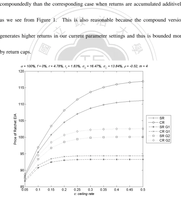
(23) contract features and model parameters may affect the value of the contract. For each set of parameters we examine six product specifications: •. SR: Simple version of Ratchet EIAs. •. CR: Compound version of ratchet EIAs. •. SR G1: Simple version of Ratchet EIAs with G1 averaging scheme. •. CR G1: Compound version of ratchet EIAs with G1 averaging scheme. •. SR G2: Simple version of Ratchet EIAs with G2 averaging scheme. •. CR G2: Compound version of ratchet EIAs with G2 averaging scheme. 立. 政治大. ‧ 國. 學 ‧. 4.2.1 Impact of return cap. Nat. The. io. sit. y. The value of the contract with various return cap shows in Figure 1.. er. contract value increases with the return cap, as expected, because capping the return. al. n. v i n C htruncates the upsideUpotential. The value increases that can be credited to the contract engchi at a diminishing rate (i.e., all curves are concave).. This is reasonable because the. probability of hitting the upper bound decreases at an increasing rate when the upper bound rises as long as the probability density of positive returns is a decreasing function of returns. We further observe that the impact of return cap is the most significant when there is no return averaging and is the least significant when returns are averaged by the first type of scheme.. The underlying reason is that the first type 23.

(24) of averaging scheme has the most significant averaging effect.. It averages over. non-overlapping sub-periods while the second type averages on cumulative returns of sub-periods.. The stronger return averaging effect decreases the probability of hitting. the upper bound more and thus reduces the impact of return cap. The impact of return cap is more significant when returns are accumulated compoundedly than the corresponding case when returns are accumulated additively as we see from Figure 1.. 政治大. This is also reasonable because the compound version. 立. generates higher returns in our current parameter settings and thus is bounded more. ‧. ‧ 國. 學. io. sit. y. Nat. n. al. er. by return caps.. Ch. engchi. i n U. v. Figure 1: Impact of Return Cap c. 24.

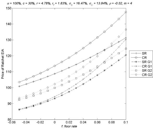
(25) 4.2.2 Impact of Return Floor Rate The value of the contract increases with the return floor as Figure 2 shows. The impact of return floor is more significant when returns are accumulated compoundedly than the corresponding case when returns are accumulated additively.. 立. 政治大. ‧. ‧ 國. 學. n. er. io. sit. y. Nat. al. Ch. engchi. i n U. v. Figure 2: Impact of return floor rate f We observe that return floor has the least impact on the contract without return averaging and has the greatest impact on the contract with the G1 averaging, given the same way of return accumulation. More specifically, the percentage change of the contract value given a change in the return floor is the smallest when there is no return. 25.

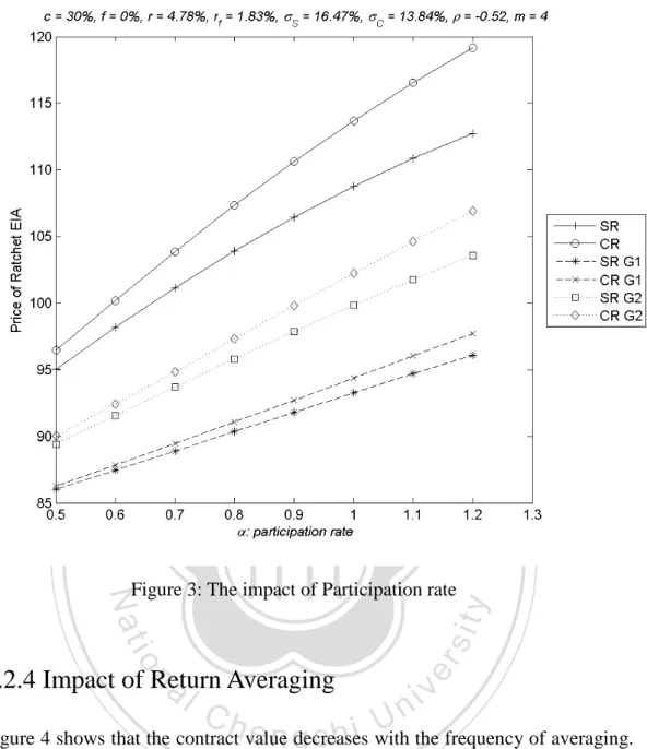
(26) averaging and is the largest when returns are averaged by the first type of scheme. The underlying reason is that the value contributed by the return volatility decreases with the floor rate.. The reduction in the contract value due to the volatility. dampening of return averaging thus decreases with the floor rate as well.. Therefore. we observe that the value increase the fastest/slowest with the floor rate for the contract with the strongest/weakest return averaging scheme.. 政治大. 立 4.2.3 Impact of Participation Rate. ‧ 國. 學. The value of the contract increases with the participation rate as Figure 3 shows. It. ‧. is interesting to seeing that the contract value is nearly linear function of participation 1.2. Also, the impact of participation rate is more significant. y. α ≤. io. sit. ≤. Nat. rate for 0.5. er. when returns are accumulated compoundedly than the corresponding case when. al. n. v i n C hBesides, the participation returns are accumulated additively. has the greatest impact engchi U. on the contract with no return averaging but has the least impact on the contract with the G1 averaging scheme.. The rationale is that the participating rate. amplifies/condenses the effect of return averaging since it is the multiplier to the annual return in equation (4).. The reduction in the contract value due to return. averaging thus increases with the participating rate.. 26.

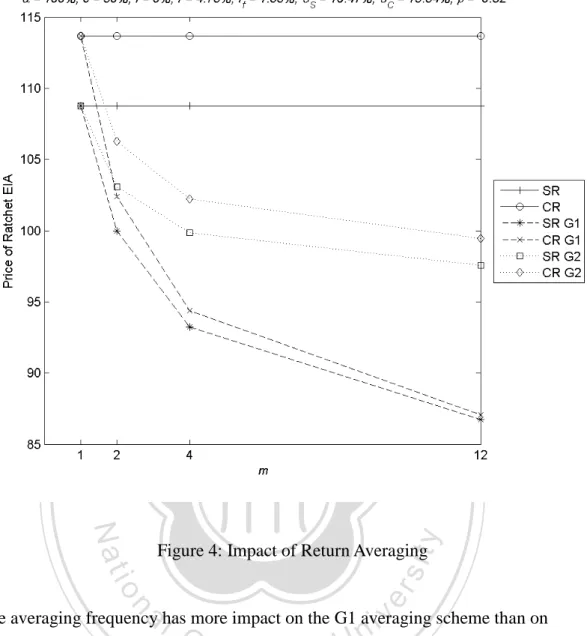
(27) 立. 政治大. ‧. ‧ 國. 學. 4.2.4 Impact of Return a Averaging. er. io. sit. y. Nat. Figure 3: The impact of Participation rate. n. iv l C n U the frequency of averaging. h e n gdecreases Figure 4 shows that the contract value c h i with The impact of return averaging can be rather significant.. The frequency of return. averaging would decrease the contract value because higher frequencies produce stronger averaging effects and reduce the volatilities of annual returns. The reduced volatilities decrease the value of the options embedded in the ratchet EIA products. The impact of return averaging is more significant for the compound version than for the simple version. 27.

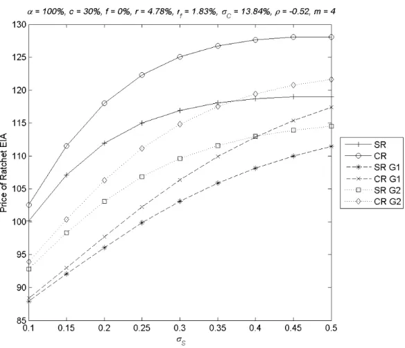
(28) 立. 政治大. ‧. ‧ 國. 學 y. Nat. n. al. er. io. sit. Figure 4: Impact of Return Averaging. i n U. v. The averaging frequency has more impact on the G1 averaging scheme than on G2.. Ch. engchi. Remember that G1 averages returns over non-overlapping sub-periods while G2. averages on cumulative returns of sub-periods.. The marginal effect of increasing the. number of sub-periods is thus larger for G1.. 4.2.5 Impact of the Volatility of Linked Index The value of the contract increases with the volatility of the linked index as Figure 5 shows. The impact of with the volatility of the linked index is also more significant 28.

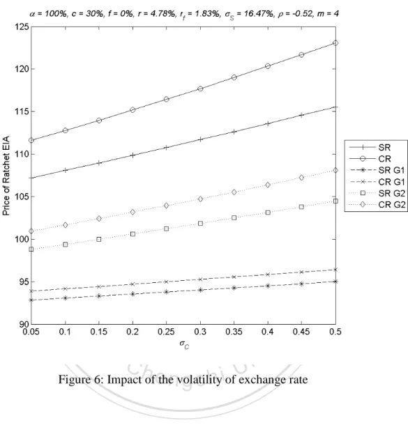
(29) when returns are accumulated compoundedly than the corresponding case when returns are accumulated additively. When the volatility of the linked index is greater than 30%, the increase in contract value of SR and CR becomes very minor. This is because the annual return is capped at 30%.. 立. 政治大. ‧. ‧ 國. 學. n. er. io. sit. y. Nat. al. Ch. engchi. i n U. v. Figure 5: Impact of the volatility of the linked index. 4.2.6 Impact of the Volatility of Exchange Rate The value of the contract increases with the volatility of exchange rate as Figure 6 shows. It is interesting to seeing that the contract value is nearly linear function of the 29.

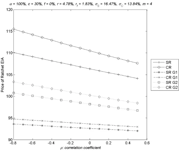
(30) volatility of exchange rate. The impact of the volatility of exchange has no big difference for CR and SR versions.. 立. 政治大. ‧. ‧ 國. 學. n. er. io. sit. y. Nat. al. Ch. engchi. i n U. v. Figure 6: Impact of the volatility of exchange rate. 4.2.7 Impact of the correlation coefficient of log(S(t)) and log(C(t)) The value of the contract decrease with the correlation coefficient of log(S(t)) and log(C(t)) as Figure 7 shows. It is interesting to noting that the contract value is nearly linear function of the correlation coefficient of log(S(t)) and log(C(t)). The impact of 30.

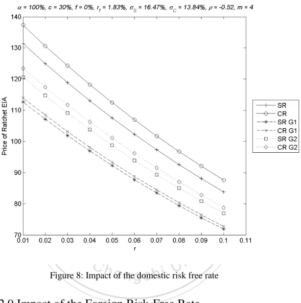
(31) ρ has no big difference for CR and SR versions. Please note that ρ = 0 is corresponding to the “non”-quanto case. From Figure 7, it is clear that the contacts are mispriced if the quanto feature has been ignored.. 立. 政治大. ‧. ‧ 國. 學. n. er. io. sit. y. Nat. al. Ch. engchi. i n U. v. Figure 7: Impact of the correlation coefficient of log(S(t)) and log(C(t)). 4.2.8 Impact of the Domestic Risk-Free Rate The value of the contract decreases with the domestic risk-free rate as Figure 8 shows, because the present value of the cash flow at maturity is a decreasing function of the domestic risk-free rate. The curves show little convexity since the contract maturity is 31.

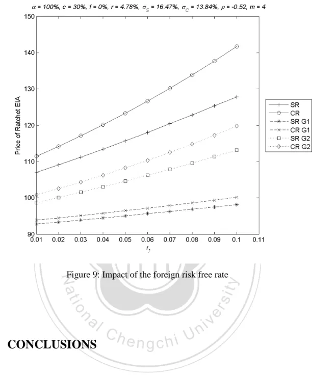
(32) merely 5 years.. The impacts of r on the contract values look to be similar across. return accumulation methods and return averaging schemes.. 立. 政治大. ‧. ‧ 國. 學. n. er. io. sit. y. Nat. al. Ch. engchi. i n U. v. Figure 8: Impact of the domestic risk free rate. 4.2.9 Impact of the Foreign Risk-Free Rate The value of the contract increases with the foreign risk-free rate at a moderately increasing speed as Figure 9 shows. This effect is the most appearing when there is no return averaging and is the least significant with the G1 return averaging.. Figure 9. further shows that the differences in the contract values between the compound and simple versions increase with the foreign risk-free rate. 32.

(33) 立. 政治大. ‧. ‧ 國. 學. n. al. er. io. sit. y. Nat. Figure 9: Impact of the foreign risk free rate. 5. CONCLUSIONS. Ch. engchi. i n U. v. Equity-indexed annuities are one innovative product brought into the insurance market recently and the sales have been growing rapidly.. Among several product. designs of EIAs, ratchet EIAs are the most popular probably because returns are credited periodically with a guaranteed minimum and the account value never decreases once the return is credited. Pricing ratchet EIAs is, however, challenging. 33.

(34) due to the complex contract features and payoff structures.. For instance, Hardy. (2004) claimed that the value of the simple version of ratchet EIAs is not analytically tractable.. Kijima and Wong (2007) could not obtain closed-form solutions for the. compound version with a return cap either. Our major contribution in this dissertation is that we derive the pricing formulas for various ratchet EIA contracts under the Black-Scholes assumptions.. 政治大. formulas cover both simple and compound versions of ratchet EIAs.. 立. Our. They may have. a return cap and can adopt either no return averaging or two types of averaging. ‧ 國. 學. schemes.. The broader coverage of our closed-form solutions make the analyses of. ‧. various contract features easier than the numerical methods provided by the literature.. Nat. io. sit. y. Our pricing formulas will be a useful tool for actuaries to design ratchet EIA contracts. er. in terms of controlling guarantee costs and market variable risks such as interest rate. al. n. v i n C hThe numerical analyses level and linked-index’s volatility. e n g c h i U using these formulas can further assist actuaries to evaluate how contract features such as return cap, return averaging, and return accumulation affect the contract value.. Our numerical results. show that the value of the contract increases with the return cap, decreases with the frequency of averaging, and is higher for the compound version.. Furthermore, the. results demonstrate that the impacts of contract features are affected by each other. The impact of return cap is the most significant when returns are accumulated 34.

(35) compoundedly and when there is no return averaging.. The impact of return. averaging is reduced significantly by return cap, and the impact of return accumulation is reduced by both return cap and return averaging.. Actuaries. therefore should always take into account contract features simultaneously when designing and managing ratchet EIA products. Our formulas will also be useful in hedging the risks of the ratchet EIA products.. 政治大. Insurers can hedge the risks introduced by embedded options using a passive. 立. approach or the dynamic-hedging approach (Boyle and Hardy, 1997).. Under the. ‧ 國. 學. passive method the insurance company offsets the liability associated with the. ‧. embedded option by purchasing appropriate options in an exchange and/or from For instance, the insurer may purchases call options. io. sit. y. Nat. another financial institution.. er. with the same underlying stock indexes in an exchange to hedge the embedded call. al. n. v i n C h These exchange-traded EIA products. engchi U. options in the ratchet. options have short. maturities only, but the insurer may roll them over to provide longer-term protections. If the insurer is concerned with the basis risk resulted from the complex contract features of the ratchet EIA products (e.g., return averaging), it may purchase average rate options in an over-the-counter market. an investment bank.. It may even arrange an equity swap with. Our formulas will help insurers to assess the due prices/costs of. the above hedging arrangements. 35.

(36) Insurers can employ our formulas in the dynamic hedging as well.. Under the. dynamic-hedging approach, the assets of the portfolio are adjusted on an ongoing basis so that the fund at maturity provides the minimum guaranteed amount when the guarantee is operative and the value of the assets otherwise.. The insurer can employ. our formulas to derive the compositions of the replicating portfolios that will be adjusted dynamically to reflect the changing indexes and time to maturity.. Due to. 政治大. the existence of transactions costs, the insurer has to adjust the replicating portfolios. 立. discretely rather than continuously and will incur hedging errors.. It therefore faces. ‧ 國. 學. the tradeoff between discrete hedging errors and transaction costs.. Hardy (2003;. ‧. chapter 8) provides detailed descriptions and assessments on this dynamic-hedging. Nat. y. Her results, in general, showed that the pricing formulas derived under. io. sit. approach.. er. simple Black-Scholes assumptions can have good hedging capacity for more general. al. n. v i n assumptions about linked-indexC and which provide another justification hinterest e n grate, chi U for using the B-S framework.. 36.

(37) References. Baxter, M., and A. Rennie. 1996. Financial Calculus: An Introduction to Derivative Pricing. Cambridge University Press. Black, F. and M. Scholes. 1973. The pricing of options and corporate liabilities. Journal of Political Economy 81: 637-654. Bjork, T. 2004. Arbitrage Theory in Continuous Time, 2nd eds. Oxford University. 立. Press.. 政治大. ‧ 國. 學. Gerber, H., and E. Shiu. 2003. Pricing lookback options and dynamic guarantees.. ‧. North American Actuarial Journal 7: 48–67.. y. sit. n. al. er. io. Colloquium.. Nat. Hardy, M. 2004. Ratchet equity indexed annuities. In 14th Annual International AFIR. Ch. i n U. v. Hardy, M. 2003. Investment Guarantees: Modeling and Risk Management for. engchi. Equity-Linked Life Insurance. Wiley. Harrison, J. M., and D. M. Kreps. 1979. Martingales and arbitrage in multiperiod security markets. Journal of Economics Theory 20: 381–408. Harrison, J. M., and S. R. Pliska. 1981. Martingales and stochastic integrals in the theory of continuous trading. Stochastic Processes and their Applications 11: 215–260.. 37.

(38) Hull, J. C. 2006. Options, Futures, and Other Derivatives Securities, 6th eds. Prentice Hall International Editions. Jaimungal, S. 2004. Pricing and hedging equity indexed annuities with Variance-Gamma deviates. Http://www.utstat.utoronto.ca/sjaimung/papers/eiaVG.pdf. Kijima, M., and T. Wong. 2007. Pricing of ratchet equity-indexed annuities under. 政治大. stochastic interest rates. Insurance: Mathematics and Economics 41: 317-338.. 立. Insurance, Mathematics, and Economics 33: 677–690.. 學. ‧ 國. Lee, H. 2003. Pricing equity-indexed annuities with path-dependent options.. ‧. Lin, S. X., and K. S. Tan. 2003. Valuation of equity-indexed annuities under. Nat. io. sit. y. stochastic interest rates. North American Actuarial Journal 6: 72–91.. er. Tiong, S. 2000. Valuing equity-indexed annuities. North American Actuarial Journal. n. al. i n C 4: 149–163; Discussions 4: 163-170 5: 128-136. h e nand gchi U. v. Vasicek, O. 1977. An equilibrium characterization of the term structure. Journal of Financial Economics 5: 177-188.. 38.

(39)