國
立
交
通
大
學
資訊科學與工程研究所
博 士 論 文
利用志願型運算
解決電腦遊戲問題
On Solving Computer Game Problems
Based on Volunteer Computing
研 究 生:林宏軒
指導教授:吳毅成 教授
利用志願型運算解決電腦遊戲問題
On Solving Computer Game Problems
Based on Volunteer Computing
研 究 生:林宏軒
Student:Hung-Hsuan Lin
指導教授:吳毅成
Advisor:I-Chen Wu
國 立 交 通 大 學
資 訊 科 學 與 工 程 研 究 所
博 士 論 文
A DissertationSubmitted to Institute of Computer Science and Engineering College of Computer Science
National Chiao Tung University in partial Fulfillment of the Requirements
for the Degree of Doctor of Philosophy
in
Computer Science
July 2013
Hsinchu, Taiwan, Republic of China
利用志願型運算解決電腦遊戲問題
研究生:林宏軒
指導教授:吳毅成 博士
國立交通大學資訊科學與工程研究所博士班
摘要
電腦遊戲是人工智慧(Artificial Intelligence)中一項非常重要的研究領域,其中有 些問題需要非常大量的運算才能解出,而志願型運算(Volunteer Computing)非常適合用 來解決這些問題。由於電腦遊戲的特性,大部份問題需要即時地產生及取消工作,這 在傳統的志願型運算上會非常沒有效率,因為傳統的志運型運算為非連線模式,無法 即時更改工作。本論文提出工作層級運算模式(Job-level Computing Model),並以此模 式為基礎發展一套新的且具有一般化之工作層級志願型運算系統,此系統使用的是連 線模式,以避免傳統志願型運算解決電腦遊戲效率不佳的問題。本論文利用傳統型志 運型運算與工作層級志願型運算分別解決兩個電腦遊戲問題:數獨最小提示數問題 (Minimum Sudoku Problem)與六子棋開局問題(Connect6 Opening Problem)。在解決數獨最小提示數問題中,本論文亦改善了 2006 年的數獨 Checker 程式, 加快了約 128 倍效率,使用此改善程式可將原本需要約 30 萬年單核時間的數獨最小提 示數問題減少成約 2417 年可解。而在解決六子棋開局問題中,成功地將證明數搜尋演 算法應用於工作層級志運型運算系統中,並提出了延遲兄弟節點產生法及假設證明數 相同之方法來展開搜尋樹節點,成功地解出許多六子棋盤面的勝敗,其中包含多個開 局,例如米老鼠開局,此開局在過去是很受歡迎的開局之一。根據實驗數據顯示,在 16 核的環境下其速率可提升 8.58 倍。
On Solving Computer Game Problems
Based on Volunteer Computing
Student:Hung-Hsuan Lin
Advisor:Dr. I-Chen Wu
Institute of Computer Science and Engineering
National Chiao Tung University
Abstract
Computer game is an important field of research in artificial intelligence, while some computer game problems take huge amount of computation time to solve, which is suitable to use volunteer computing to solve. However, due to the property of computer games, most computer game problems generate or abort jobs dynamically when solving, which makes computer game problems cannot be solved efficiently on traditional volunteer computing, which uses connectionless model and cannot support the function. This thesis proposes job-level computation model, and based on this model to propose a new generic job-level volunteer computing system, which is a connection model, to solve compute game problems efficiently. This thesis uses traditional volunteer computing and job-level volunteer computing to solve the minimum Sudoku problem and Connect6 game openings, respectively.
For solving the minimum Sudoku problem, this thesis speedups the Sudoku program Checker written by McGuire in 2006 by a factor of about 128, and reduce the computation time for solving the minimum Sudoku problem from about 300 thousand year on a one-core
machine to about 2417 years. For solving Connect6 openings, this thesis successfully incorporates proof number search into the job-level volunteering computing system, and proposes postponed sibling generation and virtual-equivalence methods to generate nodes in search trees. Based on this system, many new Connect6 game positions are solved efficiently, including several Connect6 openings, especially the Mickey-Mouse Opening, which was one of the popular openings. The experiments showed 8.58 speedups in a system with 16 cores.
致謝
經過了孜孜矻矻的多年,終於在 2013 年提出博士學位口試。 非常感謝指導老師吳毅成教授多年來的照顧,老師除了在課業及學術方面指導我 之外,更常教導我人生方面的道理,對於我在課業以外的困難更是不遺餘力地幫忙。 老師更是常利用平常假日的休閒時間指導我們,讓我們每當有問題時都能及時地與老 師討論。 感謝口試委員王才沛教授、吳毅成教授、林秉宏博士、林順喜教授、徐慰中教授、 徐讚昇教授、陳穎平教授、許舜欽教授和顏士淨教授(以上按姓氏筆劃排列),提出 論文與報告的不足之處並提出改進方法,讓我的論文與表達能更加進步。 感謝待了十年的交通大學(大學四年、研究所一年完逕博、博士五年),讓我能 順利完成學士與博士學位,也感謝在碩博六年的期間的實驗室同學兼好友們,包括林 秉宏學長、黃裕龍學長、典餘學長、RC 學長、哲毅學長、汶傑學長、冠翬、柏甫、 益嘉、聰哥、宜智、平平、賴打、小雄、gy、家茵、柏廷、郁雯、修全、tataya、正宏、 草莓、蔡心、mark、派大星、拉拉、kk、小吉、嘉嘉、青蛙、左左、piggy、東東、小 閔、TF、Miso、黑月、博玄、包子、庭築、Ting、阿賢與小康。 最後,我要感謝我最愛的父母,沒有他們就不會有我,也非常謝謝他們對於我讀 博士班的支持與鼓勵,在我遇到任何困難的時候我都可以回到溫暖的家找我父母閒聊, 在我高興的時候也能與他們分享我的喜悅,也感謝所有親戚對我的關心與支持,謹以 此論文獻給我最摯愛的家人與所有的親朋好友。 林宏軒 2013 年 7 月 22 日Contents
摘要 ... i
Abstract ... ii
致謝 ... iv
List of Figures ... vii
List of Tables ... ix
Chapter 1 Introduction ... 1
1.1 Computer Games and Computer Game Problems ... 2
1.1.1 Minimum Sudoku Problem ... 4
1.1.2 Connect6 Game Openings ... 6
1.2 Traditional Volunteer Computing ... 6
1.3 Motivation and Goal ... 8
1.4 Organization ... 11
Chapter 2 Solving Games Using BVC... 12
2.1 Introduction ... 12
2.2 Traditional Approach ... 15
2.2.1 Finding 17-clue Puzzles ... 16
2.2.2 Checking All 16-clue Puzzles ... 17
2.2.2.1. Phase 1: Unavoidable Sets and Finding Unavoidable Sets ... 18
2.2.2.2. Phase 2: Searching 𝑛-clue Puzzles ... 23
2.3 DMUS Algorithm ... 27
2.3.1 Basic DMUS Algorithm ... 28
2.3.2 Improved DMUS Algorithm ... 30
2.4 Experiment ... 33
2.4.1 The Results in Phase 2 ... 34
2.4.2 The Results in Phase 1 ... 36
2.4.3 Overall Performances ... 38
2.4.4 Different Sequences of Shrinks in the Improved DMUS Algorithm ... 39
2.4.5 Node Counts in Phase 2 ... 39
2.4.6 The Analysis of primitive grids ... 44
2.5 Conclusion ... 45
Chapter 3 Job-Level Volunteer Computing ... 47
3.1 JLVC Model ... 47
3.2 Generic Search ... 49
Chapter 4 Solving Games Using JLVC ... 53
4.1 Background ... 53
4.1.1 Proof Number Search ... 53
4.1.2 Connect6 and NCTU6 ... 54
4.2 Job-Level Proof Number Search ... 56
4.2.1 Proof/Disproof Number Initialization ... 57
4.2.2 Postponed Sibling Generation ... 58
4.2.3 Policies in the Pre-Update Phase ... 60
4.2.3.1. Virtual-Win, Virtual-Loss, and Greedy ... 61
4.2.3.2. Flag ... 63
4.2.3.3. Modified Flag ... 64
4.2.3.4. Virtual-Equivalence ... 66
4.3 Experiments ... 69
4.3.1 Experiments for Benchmark ... 72
4.3.2 The Analysis for Virtual-Equivalence ... 73
4.3.3 Flag Mechanism ... 75
4.3.4 Experiments for Difficult Positions ... 75
4.4 Discussion ... 77
4.4.1 Past Job-level-like Work... 77
4.4.2 Miscellaneous Issues ... 78
4.5 Conclusion ... 79
Chapter 5 Conclusions ... 81
List of Figures
Figure 1: (a) A 17-clue puzzle and (b) its complete grid. ... 5
Figure 2: The roles of volunteer computing ... 7
Figure 3: The complete grid with 29 17-clue puzzles. ... 17
Figure 4: Three minimum unavoidable sets. ... 19
Figure 5: Removing a region of digits, (a) one box row and (b) 2x2 boxes, from a complete grid. ... 21
Figure 6: Another solved complete grid. ... 21
Figure 7: The search tree in Phase 2 of Checker. ... 25
Figure 8: Data structures for the set of MUSs. ... 26
Figure 9: Finding the next disjoint MUS. ... 29
Figure 10: Shrink the 𝑍3 to the intersection of 𝑍3 and 𝑆. ... 31
Figure 11: The numbers of (a) visited nodes and (b) disjoint MUSs ... 40
Figure 12: (a): D3(i) (b): the ratio D3(i)/(r+1) ... 41
Figure 13: Neq,3(i) and Ngt,3(i) ... 42
Figure 14: Neq,none,4(i), Neq,shrink,4(i), Neq,prune,4(i) and Ngt,4(i) ... 43
Figure 15: The average number of children generated from each of the Neq,4(i) nodes ... 43
Figure 16: The ratio of computation time for each part compared to the average time ... 44
Figure 17: The job-level volunteer computing model ... 47
Figure 18: The messages between a client and the job-level system ... 48
Figure 19: Outline of a job-level computation model for single core ... 49
Figure 20: Outline of a job-level model ... 50
Figure 21: Expanding 𝑛3 and 𝑛 (to generate 𝑛4) simultaneously... 59
Figure 22: (a) Virtual win policy. (b) Virtual loss policy... 61
Figure 23: The pseudo code for VW, VL, and GD. ... 62
Figure 24: A starvation example for virtual-win policy. ... 62
Figure 25: The pseudo code for FG... 63
Figure 26: An example FG policy. ... 64
Figure 27: The pseudo code for MF. ... 65
Figure 28: Assign the maximal proof numbers of children for fully-flagged nodes. ... 66
Figure 29: The pseudo code for VE. ... 67
Figure 30: The search tree in Figure 28 with FG-VE policy. ... 68
Figure 32: The twelve solved openings. ... 70
Figure 33: A path in the winning tree of the Mickey-Mouse Opening. ... 71
Figure 34: The efficiencies for all 35 positions for each policy. ... 72
Figure 35: The pseudo code of counting the distance. ... 74
Figure 36: Illustrates the measurement of each distance. ... 74
Figure 37: The speedups relative to FG policy for solving 35 Connect6 positions with different policies. ... 75
Figure 38: The improvement of speedup for the most difficult 15 positions from FG to MF-VE. ... 76
List of Tables
Table 1: The complexity of computer games ... 3
Table 2: The descriptions of all versions ... 34
Table 3: The averaged time of solving one primitive grid in Phase 2 for each version ... 35
Table 4: The number of MUSs for each size found by the programs ... 37
Table 5: The averaged time of solving one primitive grid for each version ... 38
Table 6: The average solving times of using different sequences ... 39
Table 7: Game Status and the corresponding initializations. ... 57
Chapter 1 Introduction
Computer game is an important field of research in artificial intelligence, while the goal of artificial intelligence is to make computers to be more intelligent and useful. Schaeffer and Herik [45] said “chess is to AI as the fruit fly is to genetics”, which shows the importance of chess, a kind of computer game, for artificial intelligence. A milestone in the field of computer game was that Deep Blue beat the chess championship, Kasparov [10].
The research topics for computer games include solving computer games and computer game problems. However, many computer games or computer game problems difficult to solve have high complexity. The solution to solve these with low cost is to use volunteer computing. This thesis uses BOINC [5], a kind of traditional volunteer computing, to solve the minimum Sudoku problem.
However, many computer game problems cannot be solved efficiently on the traditional volunteer computing because the problems may generate or abort the jobs dynamically, which will be described in Section 1.2. Thus, this thesis also proposes a
job-level computation model. Based on this model, we propose a new generic job-level volunteer computing system [63] to solve these kind of computer game problems efficiently.
This thesis uses Connect6 openings to demonstrate the job-level volunteer computing. This chapter is organized as follows. Section 1.1 introduces computer games and computer game problems. Section 1.2 introduces traditional volunteer computing. Section 1.3 describes the motivation and goal. Section 1.4 describes the organization of this thesis.
1.1 Computer Games and Computer Game Problems
Computer games can be categorized as single player games, two-player games, and multi-player games, according to the number of players. For example, the game Sudoku, Connect6, and Mahjong are popular single player game, two-player game, and multi-player game, respectively. Also, computer games can be categorized as perfect information games, imperfect-information games, and stochastic games, according to the information obtained by each player. Each player can get all the information in a perfect information game, but some information is not available in an imperfect-information game. For example, the games Sudoku and Connect6 are perfect information games, and the game Mahjong is an imperfect-information game. Stochastic games include the element of possibility such as dice rolls.
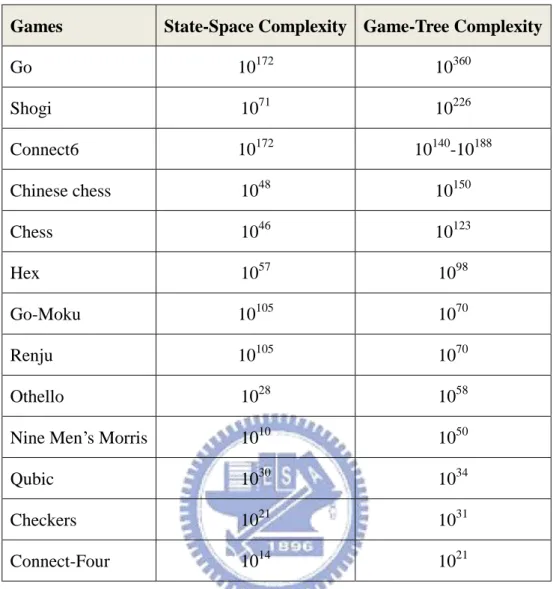
For computer games, there are two kinds of complexities to decide how hard to prove the results of the games, state-space complexity and game-tree complexity [21]. State-space complexity presents the total number of positions or states of a game. Game-tree complexity presents the number of positions needed to be evaluated in a minimax search manner [51] to determine the value of initial state of a game.
A computer game with low state-space complexity can be solved by brute-force methods, namely, by evaluating the results of all the positions in the game. And, a computer game with low game-tree complexity can be solved by knowledge-based method, namely, by heuristic searching.
Games State-Space Complexity Game-Tree Complexity Go 10172 10360 Shogi 1071 10226 Connect6 10172 10140-10188 Chinese chess 1048 10150 Chess 1046 10123 Hex 1057 1098 Go-Moku 10105 1070 Renju 10105 1070 Othello 1028 1058
Nine Men’s Morris 1010 1050
Qubic 1030 1034
Checkers 1021 1031
Connect-Four 1014 1021
Table 1: The complexity of computer games
As shown in Table 1, Go [40], Shogi [25], and Chinese chess [69] have the highest, second highest, and third highest complexity, 10360, 10226, and 10150, respectively.
Many researchers have been trying to solve computer games. Some computer games have been weakly solved since the games have low state-space complexity and game-tree complexity, such as Connect-Four [1] and Qubic [37]. Some computer games have mainly been weakly solved by brute-force methods because they have low state-space complexity, such as Nine Men’s Morris [19] and Nine-Layer Triangular Nim [49]. And, some computer games have mainly been weakly solved by knowledge-based methods, such as Go-Moku [3], Renju [57], checkers [46], and k-in-a-row games.
Unsolved and hard computer games are tournament items for computer game tournaments. For example, many computer game tournaments were held, such as TCGA Tournaments [54], TAAI Tournaments [28][70], ICGA Tournaments [24], etc, and many computer games competition were held in these tournaments, such as chess, Chinese chess, Connect6, Go, Hex, Shogi, etc.
Besides the above, there are some computer game problems, such as building the opening databases, solving the endgame positions, or some other interesting problems. Here we introduce two computer game problems which this thesis tends to solve, the minimum Sudoku problems and Connect6 game openings.
1.1.1 Minimum Sudoku Problem
Sudoku is a popular puzzle game invented by Harold Garns (cf. [33]) in 1979 and has been popular and printed in daily newspapers, magazines, and websites since 2005. A
Sudoku puzzle is played on a 9×9 grid which is divided into nine boxes each with 3×3 cells.
In a puzzle, some digits between 1 and 9 are initially given on the grid as the clues.
The aim of a Sudoku puzzle is to fill the 9×9 grid up from the initial grid of Sudoku puzzle into a valid Sudoku complete grid, or simply called a complete grid, where each column, each row and each box contains distinct digits 1-9.
(a)
(b)
Figure 1: (a) A 17-clue puzzle and (b) its complete grid.
A Sudoku puzzle is called a valid Sudoku puzzle, or simply a valid puzzle, if it is solved with a unique complete grid. A valid puzzle with 𝑛 clues initially is called an 𝑛-clue
puzzle. Figure 1 (a) illustrates a 17-clue puzzle, while Figure 1 (b) shows the complete grid
of this puzzle. And, the minimum Sudoku problem is investigating the minimum of clues for Sudoku puzzles. This thesis uses traditional volunteer computing, BOINC [5], to help solve this problem by exhaustively checking all 16-clue puzzles.
1.1.2 Connect6 Game Openings
Connect6 [61][62] is a kind of six-in-a-row game that was introduced by Wu et al. Two players, named Black and White, alternately play one move by placing two black and white stones respectively on empty intersections of a Go board (a 1919 board) in each turn. Black plays first and places one stone initially. The winner is the first to get six consecutive stones of his own horizontally, vertically or diagonally.
One issue for Connect6 is that the game lacks openings for players, since the game is still young when compared with other games such as chess, Chinese chess and Go. Hence, it is important for the Connect6 player community to investigate more openings quickly. This problem is not suitable to solve on traditional volunteer computing, and this thesis proposes job-level volunteer computing to help solve.
1.2 Traditional Volunteer Computing
As described above, some computer game problems are hard to solve and need huge amount of computing resources. Volunteer computing can be used to help solve these problems with low cost. Volunteer computing uses the spare time of computers without influencing the users’ usage. For most computers, CPU idle percentage is very high. If the idle CPU can support, then many problems can be solved. For example, BOINC [5], Berkeley Open Infrastructure for Network Computing, is a popular middleware for
volunteer computing. Many projects are running on it, such as SETI@home [6][48], Einstein@home [14], and PrimeGrid [39], etc.
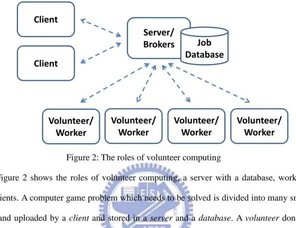
Figure 2: The roles of volunteer computing
Figure 2 shows the roles of volunteer computing, a server with a database, workers, and clients. A computer game problem which needs to be solved is divided into many small
jobs, and uploaded by a client and stored in a server and a database. A volunteer donates
spare time and helps run the jobs, which performs as a worker. These workers download jobs from the server and send the results back to the server after the jobs are completed, and the server will verify the results.
Traditional volunteer computing uses connectionless model. The workers connect to the server when they download the jobs, which can be run offline. The workers will connect to the server again when they want to upload the results and download more jobs. For example, as a worker of BOINC, the worker can download many jobs at a time which may take tens of days to run, and upload the results after completed.
The connectionless model cannot solve most computer game problems efficiently because the computer game problems are usually highly dynamic as follows. When solving the computer game problems, the result of a job may generate new jobs or abort other jobs
Server/
Brokers
Volunteer/
Worker
Volunteer/
Worker
Volunteer/
Worker
Volunteer/
Worker
Job
Database
Client
Client
and makes the jobs dynamically changes. For example, for the game Connect6, the player to move needs to consider every possible move and verify how good the moves are, and then choose the best one to move. If the player finds that one of the possible moves can get a win, then other moves can be aborted immediately. However, the traditional volunteer computing uses connectionless model and the server cannot ask the workers to abort the jobs, so the workers would waste much time on running useless jobs when solving computer game problems.
1.3 Motivation and Goal
This thesis uses volunteer computing to solve two computer game problems, the minimum Sudoku problem and the Connect6 game openings. The minimum Sudoku problem can be divided into many small independent jobs which can be run in parallel, so the problem can be solved on the traditional volunteer computing, and this thesis uses BOINC [5] to help solve.
For solving the minimum Sudoku problem, this thesis modifies the program written by McGuire in 2006 [34], and speedups the program by a factor of about 128, which reduces the computation time of solving the minimum Sudoku problem from about 300,000 one-core years to about 2417 one-core years. After improving the program, we started to solve the minimum Sudoku problem using BOINC framework [5]. At the end of July 2013, our project has completed the checking of more than 93% primitive grids, and no 16-clue grids have been found yet. We expect to complete the result soon.
Independently, McGuire also improved his own program Checker. According to his article [35], their modified Checker was about twice faster than mine and he took one whole year to run the jobs through January 2011 to December 2011. They claimed the result that
no 16-clue puzzles exist in January 2012, while our BOINC was still running at that time. Our project still continues on BOINC. At the end of July 2013, our project has completed the checking of more than 93% primitive grids, and no 16-clue grids have been found yet. We expect to complete the result soon.
Another problem this thesis uses volunteer computing to solve is the Connect6 game openings. However, as described above, the problem of solving Connect6 game openings is highly dynamic and cannot be solved efficiently on the traditional volunteer computing. Thus, this thesis proposes a new generic job-level volunteer computing system, which is connection model, to help solve the problem efficiently. This thesis introduces a new approach, named generic job-level search, where a search tree is maintained by the client. Search tree nodes are evaluated or expanded/generated by leveraging the game-playing programs which are already well-written and encapsulated as jobs, usually heavy-weight jobs requiring tens of seconds or more. The generic job-level search approach also has the following advantages:
Develops jobs (usually heavy-weight jobs or well-written programs) and the job-level search independently, except for a few extra processes required to support job-level search from these jobs. As described in this thesis, these processes are relatively low-level.
Dispatches jobs to remote processors in parallel. Job-level search is suited to parallel processing since the jobs are heavy-weight.
Maintains the job-level search tree inside the memory of clients without much problem. Since well-written game-playing programs normally support accurate domain-specific knowledge to a certain extent, the search trees require fewer nodes to solve the game positions (when compared with a best-first search such as proof number search [4] using one process only). In our experiments for Connect6, the search tree usually
contains no more than one million nodes, which fits well into (client) process memory. For example, assume that it takes one minute to run a job (to generate one node). A parallel system with 60 processors takes about 11 days to build a tree of up to one million nodes. Should we need to run much more than one million nodes, we can split the job-level search tree into several nodes, each per client.
Easily monitors the search tree. Since the maintenance cost for the job-level search tree is low, the client that maintains the job-level search tree can support more GUI utilities to let users easily monitor the running of the whole job-level search tree in real time. In fact, our client is embedded into a game record editor environment. An extra benefit of this is to allow users or experts to look into the search tree during the running time, and to help choose the best move to search in the case that the program does not find the best move to win (see [59][65]).
For node generation of generic job-level search, we need to select nodes and then expand them. For node expansion, this thesis proposes a method, named postponed sibling
generation method, to help expand the selected nodes.
This thesis also proposes a new policy, named virtual-equivalence. In this policy, it is assumed that the value of a game position is close to (or equal to) that of the position for the best move, and that the value for the 𝑛th best move is close to (or equal to) that for the (𝑛 + 1) best move. This thesis also proposes some variants of virtual-equivalence. The experiments showed that one of the virtual-equivalence variants performed the best and improved the virtual-win/virtual-loss policies by a factor of about 1.86.
Using proof number search to maintain the search tree with the job NCTU6, on desktop grids (a kind of volunteer computing system1 [5][16][48][59]), this thesis solved
1 A desktop grid is developed for volunteer computing which aimed to harvest idle computing resources for
several Connect6 positions including several difficult 3-move openings, as shown in Figure 32 (in Section 4.3). For some of these openings, none of the human Connect6 experts had been able to find the winning strategies. These solved openings include the popular
Mickey-Mouse Opening2, [55], as shown in Figure 32 (i).
1.4 Organization
The organization of this thesis is as follows. Chapter 2 uses traditional volunteer computing, BOINC [5] volunteer computing (BVC), to solve the minimum Sudoku problem. Chapter 3 defines job-level volunteer computing (JLVC). Chapter 4 uses JLVC to solve Connect6 game openings. Chapter 5 concludes this thesis.
2 The opening was so called by Connect6 players since White 2 and Black 1 together look like the face of
Chapter 2 Solving Games Using BVC
The first problem this thesis tends to solve is: what is the minimum number of clues for a valid Sudoku puzzle? This is the so-called minimum-clue Sudoku problem, or the
minimum Sudoku problem.
Since this problem can be divided into many small jobs, which can be run independently, this problem is suitable to be solved on the traditional volunteer computing. This thesis uses BOINC [5] volunteer computing (BVC) to help solve this problem.
This chapter is organized as follows. Section 2.1 introduces this problem. Section 2.2 describes traditional approaches for the minimum Sudoku problem including the program Checker [34]. Section 2.3 describes our new approach. Section 2.4 does experiments for analyzing the performance improvements by our approach. Section 2.5 makes concluding remarks.
2.1 Introduction
The minimum Sudoku problem is asking for the smallest 𝑛 for valid 𝑛-clue puzzles. Currently, many 17-clue puzzles have been found. One of these puzzles is shown in Figure 1 (a). The approach to solving the problem is briefly described as follows.
For a given grid, we can easily generate more isomorphic grids [42] by the following operations.
Relabel digits. For example, relabel all 2s and 5s to 5s and 2s, respectively.
Permute single rows (columns) within the same box row (column), or permute box rows (columns). A box row (column) indicates the three boxes in the same rows
(columns). For example, permute the first and second rows; permute the first box column (the leftmost three boxes) and the second box column (the middle three boxes). Rotate and mirror boards.
An important assertion is: if a puzzle 𝑃 with initial grid 𝐺 is valid, then another puzzle 𝑃' with initial grid 𝐺' which is isomorphic to 𝐺 is valid, too. The puzzle 𝑃' is said to be isomorphic to 𝑃. For simplicity of discussion, let 𝑖𝑠𝑜(𝐺) denote the group of
isomorphic grids generated from 𝐺. Note that 𝐺 is also included in 𝑖𝑠𝑜(𝐺). From above,
if a puzzle with initial grid G is valid, all the puzzles with initial grids in 𝑖𝑠𝑜(𝐺) are valid too.
The numbers of isomorphic grids in groups are usually enormous. For example, a complete grid may have up to 2*9!*68 = 1,218,998,108,160 isomorphic complete grids.
Similarly, a valid puzzle such as the one in Figure 1 (a) normally has enormous isomorphic valid puzzles, too. Thus, it becomes less interesting to find valid puzzles which are isomorphic to some found valid puzzles. Currently, Royle [41] collected 49151 17-clue puzzles, each of which is not isomorphic to any others. These puzzles are called essentially
different Sudoku puzzles.
The total number of complete grids is 6,670,903,752,021,072,936,960 [17]. In fact, many of them are isomorphic. The total number of distinct isomorphic groups is 5,472,730,538 [42]. Fowler [18] also generated 5,472,730,538 complete grids, one for each isomorphic group. These complete grids are essentially different Sudoku grids, and are called primitive grids in this thesis. Two features of primitive grids are as follows.
1. Each complete grid is isomorphic to one of these primitive grids. 2. Each primitive grid is not isomorphic to any other primitive grids.
An important approach to solving the minimum Sudoku problem is investigating exhaustively all these primitive grids only to check whether 16-clue puzzles exist in these
primitive grids or not. The approach must be able to find one 16-clue puzzle, if there exists a 16-clue puzzle, for the following reason. Assume that some 16-clue puzzle 𝑃 can be solved with a unique complete grid 𝐺. From the first feature, there exists one and only one primitive grid 𝐺', isomorphic to 𝐺. This implies that there exists a 16-clue puzzle 𝑃' solved with the complete grid 𝐺' uniquely. Namely, we can translate the initial grid of puzzle 𝑃 into that of 𝑃' by using the same transformation from 𝐺 to 𝐺'. Thus, the puzzle 𝑃' should be found when the primitive grid 𝐺' is investigated.
Using this approach, McGuire [34] wrote a program, named Checker, in 2006 to help solve this problem. Given a number 𝑛 and a complete grid, the program checks whether there exist 𝑛-clue puzzles which can be solved with the complete grid, and outputs the found 𝑛-clue puzzles, if any. Hence, we can solve the minimum Sudoku problem by using Checker to search 16-clue puzzles from all the 5,472,730,538 primitive grids.
This approach has two advantages. First, the program does not need to investigate isomorphic complete grids redundantly. Second, these primitive grids can be checked independently. That is, they can be done on top of traditional volunteer computing, such as BOINC volunteer computing [5].
Unfortunately, the total computation time for solving the problem is still too high. According to our experiment (see Section 2.4), the program Checker written in 2006 actually required on the average about 1792.31 seconds to check a primitive grid on one core of a computer equipped with the CPU, Intel(R) Xeon(R) E5520 @ 2.27GHz. Thus, for 5,472,730,538 primitive grids, it would take about 311,000 years. The total time was unfortunately too long.
In this thesis, we propose a new approach to improve the program Checker. We design a new algorithm, named DMUS algorithm [29], incorporate it into the program Checker, and make some more tunings on the program. According to our experiment (see Section
2.4), the modified program could check one on the average on one core of a computer in 13.93 seconds. Thus, it would only take about 2417 years to check all 5,472,730,538 primitive grids.
Since the 5,472,730,537 primitive grids are independent, we can have many independent jobs to run on traditional volunteer computing, such as BOINC. We started our Sudoku project to solve the minimum Sudoku problem on BOINC on October 2010. At the end of July 2013, the Sudoku project has completed the checking of more than 93% primitive grids, and no 16-clue grids have been found yet. We expect to complete the result soon.
McGuire, the author of the program Checker, with his team also improved their own program independently. According to their article [35], their modified Checker was about twice faster than mine and he took 7.1 million core hours on the Stokes machine, an SGI Altix ICE 8200EX cluster with 320 compute nodes, to solve the minimum Sudoku problem. They started running the jobs in January 2011, finished in December 2011, and claimed the result that no 16-clue puzzles exist in January 2012. In contrast, our first paper was submitted to TAAI in June 2010 [30] and we started running jobs in October 2010. Although the minimum Sudoku problem was solved by McGuire in January 2012, we still continued our project because our independent program can also help verify the result.
2.2 Traditional Approach
Solving the minimum Sudoku problem is a very difficult job as described above. Most researchers tend to seek 16-clue or 17-clue puzzles at random, instead of searching all cases exhaustively. In case that there exists some 16-clue puzzle, the 16-clue puzzle implies the existence of another 65 17-clue puzzles by simply filling one more cell on the 16-clue
puzzle. On the other hand, if one of the 65 17-clue puzzles is found, then we can easily find the 16-clue puzzle by removing one clue and checking whether or not it is still valid. Most researchers seek 17-clue puzzles in this approach.
In the rest of this section, Subsection 2.2.1 describes the traditional approaches of finding more 17-clue puzzles, while Subsection 2.2.2 describes the traditional approaches of checking whether or not 16-clue puzzles exist.
2.2.1 Finding 17-clue Puzzles
One of the most popular algorithms of finding new 17-clue puzzles is called gene
restructuring in [23][32]. This algorithm starts with an 𝑛-clue puzzle and then performs the
following operation. First, remove 𝑝 existing clues on the puzzle, and then add 𝑞 clues back to the puzzle. For simplicity, let – 𝑝 + 𝑞 indicate such an operation.
We introduce two common methods from the Sudoku Forum [53] to obtain more 17-clue puzzles from the existing valid puzzles as follows:
1. Do −𝑘 + 𝑘 operations from 17-clue puzzles.
2. Do the following from 𝑛-clue puzzles, where 18 𝑛 23.
a. Repeat −2 + 1 operations until 18-clue puzzles are obtained.
b. Then, repeat −1 + 1 operations many times to obtain more 18-clue puzzles. c. Finally, do one −2 + 1 operation to obtain more 17-clue puzzles.
The first method starts with 17-clue puzzles and does a −𝑘 + 𝑘 operation to obtain new 17-clue puzzles. Running with 𝑘 2 is very fast, while it takes much longer time with 𝑘 ≥ 4.
The second method starts with 𝑛 -clue puzzles where 18 𝑛 23 , and repeats −2 + 1 operations until it gets 18-clue puzzles. Also it does an extra −1 + 1 operation many times on the 18-clue puzzles to obtain more 18-clue puzzles. Finally, a −2 + 1
operation is used on these 18-clue puzzles to get 17-clue puzzles.
Both methods above are very useful to find 17-clue puzzles. Many of the 49151 17-clue puzzles were obtained in this way. However, since no 16-clue puzzles were found, they failed to conclude whether or not any 16-clue puzzles exist.
2.2.2 Checking All 16-clue Puzzles
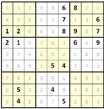
Another approach to solving the minimum Sudoku problem is to exhaustively search for 16-clue puzzles. This can be done by the program Checker [34], written by McGuire in 2006. This program was motivated when Royle (cf. [34]) found a special complete grid shown in Figure 3, where we can find exactly 29 17-clue puzzles. That is, these 29 17-clue puzzles can be solved uniquely with this complete grid. Since a 16-clue puzzle could produce 65 17-clue puzzles as describe above, it is more likely that this complete grid contains a 16-clue puzzle, though no other 16-clue puzzles have been found from this puzzle by Checker.
Given a complete grid and a number 𝑛, the program Checker runs in the following two phases. Phase 1 is to search the grid for unavoidable sets, defined in Subsection 2.2.2.1. Phase 2, described in Subsection 2.2.2.2, uses these unavoidable sets to search 𝑛-clue puzzles.
2.2.2.1. Phase 1: Unavoidable Sets and Finding Unavoidable Sets
In a complete grid, an unavoidable set is a set of cells on which the digits can be permuted to form another distinct complete grid. In other words, if we remove all the digits in an unavoidable set from the complete grid and let the remaining digits form a new puzzle, then the new puzzle can be solved with more than one complete grid. For example, for a complete grid including the bolded digits shown in Figure 4, the four bolded digits, two 1s and two 2s, in the upper left corner form an unavoidable set. The complete grid is transformed to another complete grid by exchanging the 1s and 2s in this unavoidable set. In fact, all bolded 4s and 5s form one unavoidable set; all bolded 6s, 7s, 8s and 9s form one; and all of these 1s, 2s, 4s and 5s also form one. From the definition, we have the following assertion, which is important in Phase 2 of Checker.
Figure 4: Three minimum unavoidable sets.
Assertion 1. Assume 𝑃 to be a valid puzzle uniquely solved with a complete grid 𝐺. For each unavoidable set in 𝐺, at least one of the cells in the unavoidable set must be a clue in 𝑃. ▌
An unavoidable set 𝑆 is called a minimal unavoidable set, or simply called a MUS in this thesis, if there exist no other smaller unavoidable sets 𝑆' ⊂ 𝑆. For example, in Figure 4, there are three MUSs: one with all bolded 1s and 2s, one with all bolded 4s and 5s, and one with all bolded 6s, 7s, 8s and 9s. The unavoidable set with all bolded 1s, 2s, 4s and 5s is not a MUS. In this example, the smallest size of MUSs is four and the second smallest size is six. In fact, four is also the smallest size among all MUSs.
Here, we introduce two approaches used in Checker to find MUSs from a complete grid in the following two subsections respectively.
Remove-Region Approach
The first, called the remove-region approach, is to quickly find the MUSs in a designated region of a complete grid. This approach is performing the following four steps. 1. Remove the digits from the designated region of a complete grid 𝐺, and let the
remaining digits form a new puzzle 𝑃.
2. Use a solver to solve 𝑃, producing many complete grids.
3. For each of the solved complete grids, the cells with different digits from those in 𝐺 form an unavoidable set.
4. Among these found unavoidable sets, keep the minimum ones (MUSs).
(b)
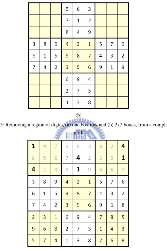
Figure 5: Removing a region of digits, (a) one box row and (b) 2x2 boxes, from a complete grid.
Figure 6: Another solved complete grid.
Let us illustrate the approach by the complete grid, denoted by 𝐺, shown in Figure 1 (b). By using the approach, remove the upper box row (the upper three boxes) from the
complete grid 𝐺 as a puzzle as shown in Figure 5 (a). Then, use a solver to solve the new puzzle. Surely, the original 𝐺 must be one of the solved complete grids. Another one of the solved complete grids is shown in Figure 6, where the digits on the gray cells are different from those in the original 𝐺. Obviously, these gray cells form an unavoidable set, which is also a MUS since there exist no smaller unavoidable sets.
In the remove-region approach, the program Checker tried to remove three kinds of regions. The first is to remove a box row or a box column as shown in Figure 5 (a). Since there are three box rows and three box columns in a Sudoku grid, Checker needs to check six times for this kind of regions. The second is to remove 2x2 boxes as shown in Figure 5 (b). For this kind of regions, Checker needs to check nine times for a Sudoku grid. The third is to select three distinct digits, say 1, 2 and 3, and then remove all the 1s, 2s and 3s in the complete grid. For this kind of regions, Checker needs to check C(9,3) (=84) times for a complete grid.
The advantages of the remove-region approach is to find quickly all the MUSs in a designated region, regardless of the sizes of MUSs, sometimes up to 20 or more. However, the drawback of this approach is that some MUSs with small sizes cannot be found. For example, some MUSs with sizes about 10 cannot be found in this approach. Note that the search in Phase 2, described in the next subsection, performs more efficiently for smaller size MUSs.
Brute-Force Approach
The second, called the brute-force approach, uses a kind of brute-force method that is to search exhaustively all MUSs with different sizes, starting from 4 (the smallest size of MUSs). Namely, an initial set of MUSs with different sizes is prepared in advance, such as the one with all 1s and 2s in Figure 4. For each of these MUSs, the method checks all of its
isomorphic to another MUS, if both are the same after we relabel digits and rotate/mirror columns or rows of one like those described in the beginning of this chapter. Surely, the MUSs in the initial set are not isomorphic to one another.
The advantage of the brute-force approach is that one can find MUSs with small sizes that cannot be found in the above approach. In Checker, most MUSs3 with sizes 12 or less were prepared in this approach.
The drawback of the approach is that checking all the isomorphic MUSs performs inefficiently since one MUS has many isomorphic MUSs but a complete grid contains only a few of them. Since Checker took much longer times in Phase 2 (about 1754.89 seconds for a primitive grid, described in greater details in Section 2.4), the overhead incurred by the brute-force becomes negligible. Thus, the brute-force approach is also used in Checker.
2.2.2.2. Phase 2: Searching 𝒏-clue Puzzles
Phase 2 is to use a tree search to find 𝑛-clue puzzles based on the MUSs found. By Assertion 1 described above, for each MUS, at least one clue in a valid puzzle must be located on one of cells in the MUS. Thus, given a number 𝑛, a complete grid 𝐺, and a set of MUSs, the program Checker in this phase is to find 𝑛-clue puzzles by recursively calling the tree search routine, named ProcessTuple(𝑛, 𝐺, 𝑋𝑐𝑢𝑟, 𝐶), where 𝑋𝑐𝑢𝑟 is the set of active MUSs and 𝐶 is the set of clues being chosen. A MUS is called active in this thesis, if none of cells in the MUS are chosen as clues (in 𝐶) yet, and inactive, otherwise. Initially, all MUSs are viewed as active MUSs, and there are no clues initially. The routine is described as follows.
Routine ProcessTuple(𝑛, 𝐺, 𝑋𝑐𝑢𝑟, 𝐶):
3 Checker prepares 47 kinds of MUSs for size 10, 44 for size 11, and 417 for size 12 in the initial set
1. If there exists at least one active MUS in 𝑋𝑐𝑢𝑟, do the following.
a. If the number of clues, denoted by |𝐶|, is already 𝑛, return without any puzzles found.
b. If |𝐶| < 𝑛, find the active MUS, 𝑆, with the smallest size of cells. For each cell 𝑐 in 𝑆, do the following.
i. Choose 𝑐 as a clue, and add it into 𝐶.
ii. Update 𝑋𝑐𝑢𝑟 according to 𝑐. Namely, remove all active MUSs containing 𝑐 from 𝑋𝑐𝑢𝑟.
iii. Recursively call the routine.
2. If there exists no active MUSs, that is, the set 𝑋𝑐𝑢𝑟 is empty, do the following. a. If |𝐶| = 𝑛, check whether the puzzle with these 𝑛 clues is valid or not. If valid,
return this puzzle, an 𝑛-clue puzzle. If not, simply return without any puzzles found.
b. If |𝐶| < 𝑛, repeatedly perform the operations 1.b.i to 1.b.iii for each non-clue 𝑐 ∉ 𝐶 on the grid 𝐺.
At Step 1, the routine checks whether there exists at least one active MUS in 𝑋𝑐𝑢𝑟, and performs, if so, the substeps 1.a and 1.b as follows. Consider the case that the routine has chosen 𝑛 clues and at least one of MUSs is still active, not containing any clues. Then, the chosen 𝑛 clues do not form a valid puzzle according to the Assertion 1. Thus, no more search is required, as described in Substep 1.a.
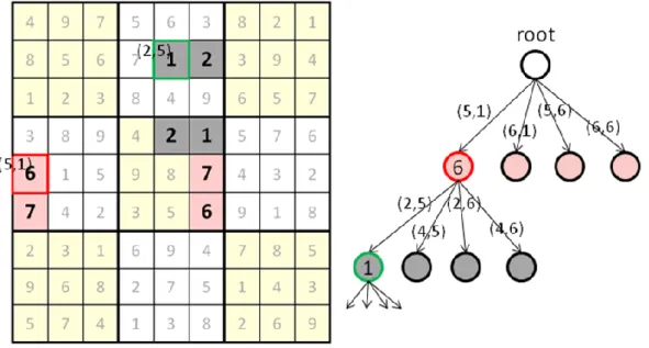
Figure 7: The search tree in Phase 2 of Checker.
In the case that the routine has chosen less than 𝑛 clues (as described in Substep 1.b), choose one MUS 𝑆 for further search. For each cell in 𝑆, add it into 𝐶, update the set of MUSs 𝑋𝑐𝑢𝑟 accordingly, and search more 𝑛-clue puzzles by recursively calling the routine itself. Note that the routine chooses the MUS with the smallest size of cells, since the one with less cells will expand a less number of subtrees. For example, in the complete grid given in Figure 7, if the cell with digit 6 at (5, 1)has been chosen, the routine finds another MUS with size 4 next, marked as gray in the figure, chooses one of these cells in the MUS as a clue, say the cell with digit 1 at (2, 5), and then recursively calls the routine to find more.
At Step 2, the routine performs Substeps 2.a and 2.b when no more active MUSs exist. In the case that the routine has chosen 𝑛 clues (Substep 2.a), a solver is used to check whether the puzzle with the 𝑛 clues is valid. If the puzzle can be solved with at least two distinct complete grids, the solver reports invalid. Otherwise, the solver reports valid, that is, a puzzle with 𝑛 clues is found.
In the case that the routine has chosen less than 𝑛 clues (Substep 1.b), it becomes more promising to find 𝑛-clue puzzles. In this case, we need to check all non-clue cells by
recursively performing the operations 1.b.i to 1.b.iii to search all 𝑛-clue puzzles.
The above routine needs to maintain the set of active MUSs efficiently. The maintenance includes the following two important operations, (a) finding the active MUS with the smallest size of cells, and (b) removing all MUSs containing a designated cell (chosen as a clue).
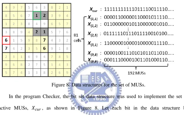
Figure 8: Data structures for the set of MUSs.
In the program Checker, the bit set data structure was used to implement the set of active MUSs, 𝑋𝑐𝑢𝑟, as shown in Figure 8. Let each bit in the data structure be corresponding to a designated distinct MUS. Namely, the ith bit with 1 indicates the ith MUS to be inactive, while that with 0 indicates active. It is the same when switching the representation of values 0 and 1. Thus, for 192 MUSs, the default setting of Checker, the data structure requires 6 words each with 32 bits.
For operation (a), we can arrange the MUSs with small sizes to the front. For example, the MUSs with size 4, if any, are arranged to the front of bits of 𝑋𝑐𝑢𝑟. So, if we want to find the active MUS with the smallest size, we simply scan bits of 𝑋𝑐𝑢𝑟 from the front to rear and find the first bit with 0 (indicating active). For example, if there exists some active MUS with size 6 and no active MUSs with size 4, we will find a MUS with size 6 by the scanning.
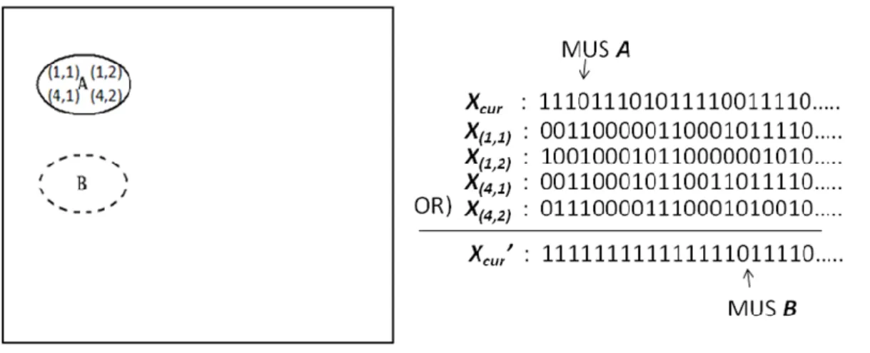
For operation (b), for each cell 𝑐, we initialize a set of MUSs 𝑋𝑐 that contain the cell 𝑐. If we choose the cell 𝑐 to be a clue, then the MUSs which contain the cell 𝑐 become all inactive. Using bit set data structure, we can easily use bitwise operations to remove the MUSs from the set of active MUSs easily. Let 𝑋𝑐 be also implemented by a bit set data structure. The ith bit in 𝑋𝑐 is set to 1 to indicate that the ith MUS contains the cell 𝑐, and 0, otherwise. For example, in Figure 8, if we choose one more cell with digit 1 at (2,5) to be a clue, 𝑋𝑐𝑢𝑟 becomes the value of performing OR operation on the original 𝑋𝑐𝑢𝑟 and 𝑋(2,5). Since a Sudoku grid contains 81 cells, only 81 𝑋𝑐 need to be initialized.
From above, it can be shown that all the 𝑛-clue puzzles, if any, can be found by Checker. In addition, some more optimizations are done by this program. For example, the same set of clues are not searched again. Namely, if the routine selects the clue at (5,1) and then at (6,1), the routine will not search again in the sequence, selecting the one at (6,1) and then at (5,1).
2.3 DMUS Algorithm
As described at the beginning of this chapter, it would take a huge amount of time to solve the minimum Sudoku problem by Checker even in the job-level computation model with a lot of resources. In this section, we design a new algorithm in Phase 2, named Disjoint MUSs (DMUS) algorithm, and tune the code to improve the performance of Checker. The details of code tuning in both two phases are omitted in this thesis. This section focuses on the DMUS algorithm. Subsection 2.3.1 proposes the basic DMUS algorithm, while Subsection 2.3.2 proposes the improved DMUS algorithm.
2.3.1 Basic DMUS Algorithm
The basic DMUS algorithm improved the program Checker by modifying Step 1.b, described in Subsection 2.2.2.2. In Step 1.b, an initial operation is added to find 𝑟 + 1 disjoint active MUSs. Let r denote 𝑛 – |𝐶|, representing the number of remaining clues to be chosen, where |𝐶| is the number of clues in 𝐶. A set of MUSs are called disjoint
MUSs, if any two of these MUSs do not overlap (namely, any two do not contain the same
cells). An important assertion related to disjoint MUSs is described as follows.
Assertion 2. Use the program Checker to find 𝑛-clue puzzles as described in Subsection 2.2.2.2. If there exists at least 𝑟 + 1 disjoint active MUSs as above, then there exist no 𝑛-clue puzzles with 𝐶4. ▌
From Assertion 1 in Subsection 2.2.2.1, for each MUS, a valid puzzle must include at least one clue in the MUS. Since there exist at least 𝑟 + 1 disjoint active MUSs in addition to the clues in 𝐶, a valid puzzle with 𝐶 must also contain at least 𝑟 + 1 disjoint clues, each from one distinct MUS. Thus, the number of clues in the valid puzzle must be at least |𝐶| + (𝑟 + 1) = |𝐶| + (𝑛– |𝐶| + 1) = 𝑛 + 1. This implies that there exist no 𝑛-clue puzzles with 𝐶, that is, Assertion 2 is satisfied.
Given a set of MUSs, the problem of finding the largest number of disjoint active MUSs can be reduced to the maximum clique problem (cf. [34]). Unfortunately, the maximum clique problem is NP-complete [7]. Since it is intractable to find a maximum clique, it is also intractable to find the largest number of disjoint active MUSs via finding the maximum clique.
In the basic DMUS algorithm, we simply use a greedy algorithm to find 𝑟 + 1 disjoint active MUSs one by one without exhaustively searching all kinds of disjoint active
MUSs, such as backtracking. The algorithm repeatedly performs the following two operations until 𝑟 + 1 disjoint active MUSs are found or no more disjoint active MUSs exist.
1. Choose one additional disjoint active MUS with the smallest size in 𝑋𝑐𝑢𝑟. 2. Add the chosen MUS into the set of disjoint MUSs.
In the first operation above, we choose the one with the smallest size, since it is more likely to find 𝑟 + 1 disjoint active MUSs in this way. This operation is the same as operation 1.b in Subsection 2.2.2.2, and therefore can be implemented by using the same bit operation.
Figure 9: Finding the next disjoint MUS.
In the second operation, we add the chosen MUS, 𝑆, into the set of disjoint MUSs. We can implement it by pretending to select all cells in 𝑆 as clues. Namely, we simply remove all the active MUSs in 𝑋𝑐 from 𝑋𝑐𝑢𝑟 for all cells 𝑐 in 𝑆. Thus, all the next chosen MUSs must not contain any cells in 𝑆. For example, in Figure 9, after we find the active MUS 𝐴, we can simply update the 𝑋𝑐𝑢𝑟 by removing 𝑋𝑐 for all the four cells 𝑐 in 𝐴. Thus, the next chosen MUS must not have any intersected cells with MUS 𝐴.
In fact, the operation can be easily improved by making a union of 𝑋𝑐 for all cells 𝑐 in 𝑆 in advance. At the beginning of Phase 2 (or the end of Phase 1), for each MUS 𝑆, we
make an 𝑋𝑆 which is the value of doing the OR operation on 𝑋𝑐 for all cells 𝑐 in 𝑆. Thus for the case in Figure 9, after selecting MUS 𝐴, we can simply update 𝑋𝑐𝑢𝑟 by making one OR operation for 𝑋𝐴, instead of four 𝑋𝑐 for all cells 𝑐 in 𝐴.
In the case that 𝑟 + 1 disjoint active MUSs are found by using the above algorithm, we can prune the whole subtree, since there exist no 𝑛-clue puzzles according to Assertion 2. In the case that 𝑟 disjoint active MUSs or less are found, the program simply goes back to the normal operation 1.b (in Subsection 2.2.2.2) to traverse the whole search subtree.
2.3.2 Improved DMUS Algorithm
This subsection further improves the basic DMUS algorithm described in the previous subsection in the case that exactly 𝑟 disjoint active MUSs are found. Let the 𝑟 disjoint active MUSs be 𝑆1, 𝑆2, … , 𝑆𝑟. Combining both Assertion 1 and Assertion 2, we obtain the following assertion.
Assertion 3. Use the program Checker to find 𝑛-clue puzzles as described in Subsection 2.2.2.2. Assume one finds 𝑟 disjoint active MUSs, denoted by 𝑆1, 𝑆2, … , 𝑆𝑟, as above. An 𝑛-clue puzzle with 𝐶 must contain at least one of the cells as clues in each 𝑆𝑖 with 1 𝑖 𝑟. ▌
Based on the assertion, a straightforward search tree needs to search about 𝑖|𝑆𝑖| puzzles, where |𝑆𝑖| is the size of 𝑆𝑖. In general, the performance is related to the sizes of these 𝑆𝑖. So, if these sizes are reduced, the performance is further improved.
In this subsection, we propose a new method to reduce the size of each 𝑍𝑖, subset of 𝑆𝑖, while maintaining Assertion 4 (below), similar to Assertion 3, where 𝑍1, 𝑍2, …, 𝑍𝑟 are disjoint sets of cells, initialized to 𝑆1, 𝑆2, …, 𝑆𝑟, respectively.
Assertion 4. From above, for each set 𝑍𝑖, where 1 𝑖 𝑟, an 𝑛-clue puzzle with 𝐶 must contain at least one of the cells in the set as clues. ▌
Assertion 4 is satisfied initially from Assertion 3. The new method to reduce the size of each 𝑍𝑖 is described in the following routine.
Routine Shrink(i):
1. Let 𝑍 = (𝑍1 𝑍2… 𝑍𝑟) − 𝑍𝑖.
2. For each active MUS 𝑆 (without containing any clues in 𝐶) disjoint with 𝑍, let 𝑍𝑖 = 𝑍𝑖 𝑆.
Let us illustrate by an example in Figure 10. Assume that 𝑟 is three, and assume to find the three active disjoint MUSs 𝑆1, 𝑆2 and 𝑆3. As described above, 𝑍1, 𝑍2 and 𝑍3 are initialized to 𝑆1, 𝑆2 and 𝑆3, and Assertion 4 is satisfied initially.
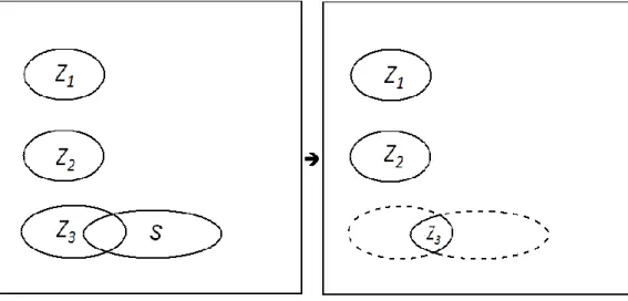
Figure 10: Shrink the 𝑍3 to the intersection of 𝑍3 and 𝑆.
Since 𝑟 is three, we need to choose three more clues, each of which must be located in 𝑆1, 𝑆2 and 𝑆3, respectively. Let us use Shrink(3) to shrink 𝑍3. In the routine, 𝑍 is initially set to 𝑍1 𝑍2. Assume that some other active MUS 𝑆 is disjoint with 𝑍 (both 𝑍1 and 𝑍2) as shown in the left of Figure 10. The set 𝑍3 is shrunk to be the intersection of the original 𝑍3 and 𝑆 as shown in the right of Figure 10.
Assertion 4 still holds for the new 𝑍3 together with both 𝑍1 and 𝑍2 for the following reason. Assume for contradiction that none of clues in an 𝑛-clue puzzle with 𝐶
are located in the new 𝑍3. From above, the clue that is located in the original 𝑍3 must be outside the MUS 𝑆. Since 𝑆 is an active MUS disjoint with both 𝑍1 and 𝑍2, none of clues are located in 𝑆. Thus, according to Assertion 1, the 𝑛-clue puzzle is not valid, contradicting the assumption. This shows that the clue in the original 𝑍3 must be in the new 𝑍3, too.
Based on the above illustration, it can be easily derived that Assertion 4 still holds after performing Shrink(i). Namely, if Assertion 4 holds currently, then it will also hold after
Shrink(i). By induction, Assertion 4 is maintained by repeatedly performing the routine Shrink.
Since the set 𝑍𝑖 may shrink after Shrink(i), it becomes very likely to shrink other 𝑍𝑗 further, where 𝑗 𝑖. Therefore, it is reasonable to repeatedly perform Shrink many times.
Many strategies can be used to perform Shrink repeatedly. For the example in Figure 10, we may choose the sequence, Shrink(1), Shrink(2) and then Shrink(3), or the sequence,
Shrink(3), Shrink(2) and then Shrink(1). We may even choose the sequence, Shrink(1), Shrink(2), Shrink(3), Shrink(2) and then Shrink(1). More discussion is given in our
experiments in Subsection 2.4.4.
In the case that some 𝑍𝑖 becomes empty after the routine Shrink(i) is finished, we can easily derive from above that none of 𝑛-clue puzzles exist. Thus, we can prune the whole subtree at Step 1.b in the routine ProcessTuple (in Subsection 2.2.2.2), like the case that we have 𝑟 + 1 MUSs. In fact, the case of 𝑟 + 1 disjoint active MUSs can be simply viewed as a special case. Let 𝑍1, 𝑍2, …, 𝑍𝑟 be the first 𝑟 disjoint active MUSs. Then, for
Shrink(r), the set 𝑍𝑟 becomes empty when choosing the last disjoint MUS 𝑍𝑟+1 as 𝑆. Namely, 𝑍𝑟 = 𝑍𝑟 𝑆 = 𝑍𝑟 𝑍𝑟+1 is empty.
In the case that none of 𝑍𝑖 becomes empty, we choose the one, say 𝑍𝑗, with the smallest size among all 𝑍𝑖, and then continue the search in the operation 1.b by using 𝑍𝑗,
instead of the original 𝑆1, the MUS with smallest size. Thus, the branching factor of the search tree becomes smaller, and therefore the size of the whole search tree is greatly reduced.
Besides the algorithm above, we also did many other tunings on the modified program. The details of these tunings are omitted in this thesis.
2.4 Experiment
We implemented the basic DMUS algorithm and the improved one as described in the previous section by modifying the program Checker. For performance analysis, all experiments were done on a personal computer equipped with the CPU, Intel(R) Xeon(R) E5520 @ 2.27GHz. In the rest of this thesis, one core indicates the above computing power.
Since it took a long time for the original program Checker to find 16-clue puzzles from one primitive grid, we only chose 100 at random among the 5,472,730,538 primitive grids (generated by the Fowler’s program [18] as mentioned above) as our benchmark for comparisons. The 100 primitive grids are listed in the webpage of the Sudoku project [52]. For simplicity of discussion, all experimental results in the rest of this section are given on the average of the chosen 100.
In the rest of this section, Subsection 2.4.1 analyzes the performance results in Phase 2 by comparing different versions of the program. Subsection 2.4.2 shows the results of the modified program in Phase 1. Subsection 2.4.3 shows the overall performance by including tuning the performances in Phase 1 of the program using different techniques. Subsection 2.4.4 compares the performances for different sequences of Shrink(i) in the DMUS algorithm. Subsection 2.4.5 shows the number of nodes in each level of Phase 2 in Checker.
2.4.1 The Results in Phase 2
In addition to the DMUS algorithm described in Section 2.3, our implementation also included many tunings, which are either omitted or briefly described due to tediousness. In this subsection, we analyze the performances of the following versions of implementations.
Version IDs Descriptions of versions
V1 Original Checker
V2 V1 with some turnings like reordering MUSs
V3 V2 with basic DMUS algorithm
V4 V3 with improved DMUS algorithm
V5 V4 with some tunings on Phase 2
V6 V5 with MUSs generated by new Phase 1 Table 2: The descriptions of all versions
As shown in Table 2, all versions are described as follows. The original version of Checker is denoted by V1. Before implementing the basic DMUS algorithm, we tuned the program by reordering the selection sequence of MUSs based on the sizes of MUSs and some other factors. After the tuning, the version is denoted by V2. The version is denoted by
V3 after incorporating only the basic DMUS algorithm into V2. Similarly, the version is denoted by V4 after incorporating only the improved DMUS algorithm into V3. Then, we made additional tunings on Phase 2 of version V4, such as reordering the sequences of MUSs and cells in MUSs during search, and the version is denoted by V5. All the MUSs used in the versions V1 to V5 were generated by the original Checker. The last version, denoted by V6, was the same as V5, except that all the MUSs were generated in Phase 1 by our modified program. Since this subsection focuses on the performances in Phase 2, the version V6 will be discussed in the next subsection, not in this subsection.
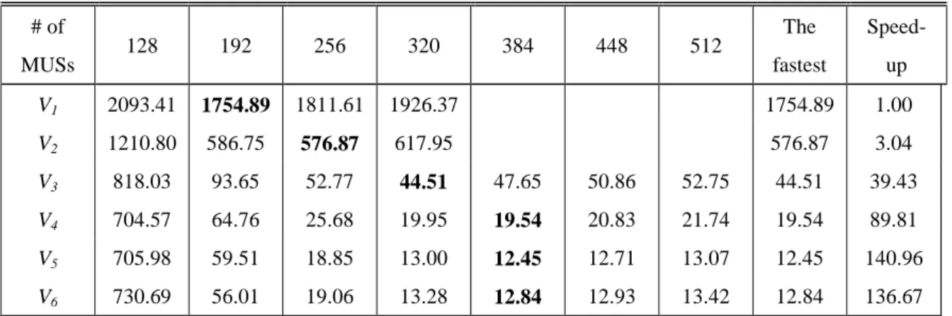
# of MUSs 128 192 256 320 384 448 512 The fastest Speed- up V1 2093.41 1754.89 1811.61 1926.37 1754.89 1.00 V2 1210.80 586.75 576.87 617.95 576.87 3.04 V3 818.03 93.65 52.77 44.51 47.65 50.86 52.75 44.51 39.43 V4 704.57 64.76 25.68 19.95 19.54 20.83 21.74 19.54 89.81 V5 705.98 59.51 18.85 13.00 12.45 12.71 13.07 12.45 140.96 V6 730.69 56.01 19.06 13.28 12.84 12.93 13.42 12.84 136.67
Table 3: The averaged time of solving one primitive grid in Phase 2 for each version Table 3 shows the averaged time of solving one primitive grid in Phase 2 in each version. In this table, we also tried different numbers of MUSs, such as 128, 192, 256, 320, 384, 448 and 512. As described above, all the MUSs used in the versions V1 to V5 were generated by the original Checker. According to our experiments, about 358.4 MUSs were generated on average for a primitive grid. The versions V1 and V2 did not run the cases for 384 MUSs or more simply because the original Checker did not support them.
In general, the more MUSs we used, the smaller search tree. Assume that more MUSs are available in Phase 2. Then, it is more likely to choose Substep 1.a to stop calling recursively. Thus, it makes the search tree smaller. Besides, more active MUSs may also help prune the search tree in our DMUS algorithm.
Searching smaller trees usually tends to raise performance, but on the other hand more MUSs may incur extra overhead. From Table 2, we observe the following: The version V1 reached the best performance for 192 MUSs, version V2 for 256, version V3 for 320, and version V4 and V5 for 384. When the numbers of MUSs decreased from the above numbers (for the best performances), the corresponding performances went down. On the other hand, when the numbers of MUSs increased from the above values, the performances went down due to the overhead incurred by the large set of MUSs.
respect to the version V1 were 3.04, 39.43, 89.81 and 140.96 respectively for versions V2 to
V5. More specifically, the DMUS algorithm improved significantly the performance by a factor of 29.54 (through V2 to V4), especially that the basic DMUS algorithm improved by a factor of 12.97 (through V2 to V3). Except the DMUS algorithm, the other tunings (through
V1 to V2 and through V4 to V5) improved by a factor of 4.77.
2.4.2 The Results in Phase 1
In this subsection, we want to discuss the experimental results in Phase 1. As described in Subsection 2.2.2.1, Phase 1 of the original Checker used both remove-region and brute-force approaches to find MUSs.
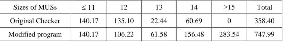
According to our experiments, for the remove-region approach, the original Checker found the MUSs in the designated regions and kept the MUSs with sizes 14 or less. The program with this approach ran very fast in about 0.5 seconds in Phase 1, and it was able to find only about 222.54 MUSs on average for a complete grid, among which 139.41 have sizes 12 or less.
In fact, the program also used the brute-force approach to search the MUSs with size 12 or less and was able to find about 358.4 MUSs on average for a complete grid, but it took much longer time, about 37.4 seconds, to find MUSs for a complete grid. Since the original Checker took a much longer time in Phase 2 (about 1754.89 as shown in the previous subsection), the computation time, 37.4 seconds, is negligible. Thus, it is more important for the program to use the above approach to find higher quality MUSs.
However, since our DMUS algorithm improves the performance significantly in Phase 2 as described in the previous subsection, the computation time for Phase 1 also becomes critical. Thus, we need to improve the performance in Phase 1. Our approach is to investigate the remove-region approach instead of the brute-force approach.