在毫微米波段下使用最佳化理論之混合式空間分割多重接取波束形成技術

國 立 交 通 大 學

電信工程學系

碩 士 論 文

在毫微米波段下使用最佳化理論之混合式

空間分割多重接取波束形成技術

Hybrid Beamforming Using Convex

Optimization for SDMA

in Millimeter Wave Radio

研究生：林科諺

在毫微米波段下使用最佳化理論之混合式空間分割多重接取波束形成技術

Hybrid Beamforming Using Convex Optimization for SDMA

in Millimeter Wave Radio

研 究 生：林科諺 Student：Ko-Yen Lin

指導教授：伍紹勳 Advisor：Sau-Hsuan Wu

國 立 交 通 大 學

電 信 工 程 學 系

碩 士 論 文

A Thesis

Submitted to Department of Communication Engineering College of Electrical and Computer Engineering

National Chiao Tung University in partial Fulfillment of the Requirements

for the Degree of Master

in

Communication Engineering September 2008

Hsinchu, Taiwan, Republic of China

在毫微米波段下使用最佳化理論之混合式空間分割多重接取波束形成技術

學生：林科諺

指導教授

：

伍紹勳 博士

國立交通大學電信工程學系﹙研究所﹚碩士班

摘

要

使用平面天線陣列來呈現射頻及基頻混合式空間分割多重接取(SDMA)

的波束形成架構，此平面天線陣列的每個單元天線都有相位移位器，把陣

列分區為許多區塊且每個區塊可共享一個數位處理路徑。為了壓抑波束圖

形的旁瓣輻射及維持使用者的訊號與干擾及雜訊比(SINR)，最佳化理論被

應用在設計此混合式空間多重接取的波束形成。兩種設計方式如下：一種

為在限制所有使用者的 SINR 下令其使用之傳送能量為最小；而另一種為在

總傳送能量限制下令其所有使用者中最差的 SINR 要最大。考慮實際上會遇

到的不同影響因素，依據此兩種設計方式，我們可以進一步的討論對於兩

個使用者的 SDMA 系統之下的混和式波束形成技術的可行性及效能。此外，

在某些程度的波束誤差下，兩種強健型波束形成技術可用來確保每個使用

者的 SINR。模擬結果顯示出，使用最佳化理論可有效改善混合式波束形成

技術的 SINR 及指向性，此外，混和式波束形成技術擁有強健性去對抗一些

延伸的影響因素，如相位變動、波束誤差及通道不確定性。

Hybrid Beamforming Using Convex Optimization for SDMA

in Millimeter Wave Radio

Student：Ko-Yen Lin

Advisor：Dr. Sau-Hsuan Wu

Department of Communication Engineering

National Chiao Tung University

ABSTRACT

A radio-frequency and baseband hybrid beamforming (HBF) scheme is

presented for spatial division multiple access (SDMA) of 60GHz applications

using planar antenna arrays (PAA). PAA with phase shifters for each element

antenna is partitioned into sub-blocks and each block is applied a common

baseband beamforming weight. To suppress the grating lobes of beam pattern

and to maintain the signal to interference plus noise ratio (SINR) of users in the

SDMA system, we study the design of this HBF using convex optimization.

Two design criteria are considered herein: one minimizes the transmit power

subject to a SINR constraint, and the other maximizes the worst case SINR

subject to a total power constraint. Based on these two criteria, the feasibility

and performance of HBF are extensively studied for a two-user SDMA system,

taking into account various factors faced in practice. Moreover, to ensure the

SINR of each user under a certain degree of beam misalignment, two robust

HBF schemes are also proposed according to the design criteria. Simulation

results show that both the SINR and directivity of HBF can be significantly

improved by making use of the convex optimization technique. In addition, the

HBF scheme is robust to some extend to phase variations, beam misalignment

and channel uncertainties.

誌

謝

能夠完成此篇論文，首先要感謝我的指導教授－伍紹勳老師，老師在

我就讀碩士班的兩年當中，很有系統地培養我成為一位研究人員，從一開

始基礎能力的訓練，到之後研究方向的找尋以及論文方法的討論，老師都

一步步耐心地從旁指導，幫助我解決問題，更在平時不斷地鼓勵我們，教

導我們正確的研究態度；在研究之餘，老師同時也很注重生活上的照顧，

將所有資源全部投注在我們身上，讓我們能夠無憂無慮的專注於研究上。

還有感謝老師的鼓勵與支持，讓我有機會可以參加國際會議，藉此增廣不

少視野。為此，在這邊深深的感謝老師。

再來，感謝 MBWCL 實驗室成員們的幫助與支持，這兩年來，實驗室

有著良好的研究環境，且大家相處的非常和樂融洽，感謝學長姊們，詔元、

晉豪、建勝及汀華，平時的照顧及熱心的回答我所遇到的疑問。感謝同屆

的同窗愈翔、沛霓、新栗，這兩年來互相的照顧和勉勵。感謝實驗室的學

弟們，人維、永宗、榮東，讓實驗室的氣氛更加活潑熱鬧，還有陪伴我一

起打籃球。接著要特別感謝俊凱、麟凱學長及縱輝博士，給我研究上的莫

大幫助，還有要感謝明虔學弟辛苦的幫忙我模擬程式，感謝各位！

最重要，要由衷感謝我的父母，辛苦提拔我至碩士畢業，有了他們在

背後默默的付出，我才有機會能順利地完成學業。最後，對所有一路陪伴

我走過來的朋友們！再次獻上我最真誠的感謝！

謝謝！

誌於 2009.10 新竹 交通大學

科諺

Contents

Contents 2

List of Figures 4

1 Introduction 1

2 The Configurations of Planar Antenna Arrays 4

2.1 SDMA using reconfigurable PAA . . . 8

3 SDMA Using Hybrid Beamforming 10 3.1 HBF based on the MD beamforming . . . 12

4 Multiuser hybrid beamforming based on convex optimization 15 4.1 HBF based on the constrained minimization of power . . . 15

4.1.1 Power minimization based on LCMP . . . 16

4.1.2 Power minimization based on SOCP . . . 17

4.2 HBF based on the constrained maximization of SINR . . . 19

5 The practical implementation for hybrid beamforming 21 5.1 The finite resolution of the phase shifters for HBF . . . 21

5.2 Robust beamforming for HBF under the steering angle mismatch . . . . 24

5.2.0.1 HBF based on the SINR constraint within a certain region 25

6 Simulation Results 33

6.1 Hybrid beamforming scheme . . . 33

6.2 Robust beamforming for HBF . . . 37

7 Conclusions 41

8 Appendix 42

List of Figures

2.1 Antenna arrays of 8 × 8 planar antennas and the position of the element

antennas with respect to the Cartesian coordinate. . . 5

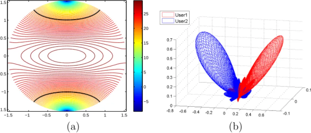
2.2 The contour plot of the antenna pattern when P=30dB and the array

factors of the 2-user SDMA based on the partition in Fig. 2.3(a). . . 6

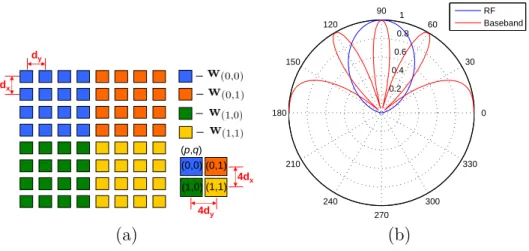
2.3 Partitions of the planar antenna arrays. Patch antennas in different color belong to different block. Polar plot of the beamforming pattern of the

hybrid scheme in PAA when θ = π/2. . . . 7

3.1 Configurations of the rearranged planar antenna arrays respect to base-band beamforming weights and polar plot of the beamforming pattern of

the hybrid scheme in rearranged PAA when θ = π/2. . . . 12

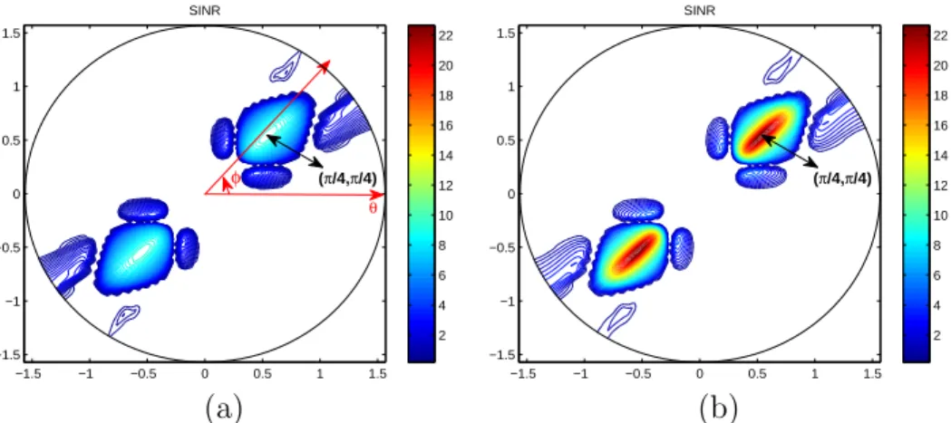
6.1 The contour plots of SINR for user 1, using the RF beamforming and the HBF of LCMP, with the desired directions of user one and two set at

(φ1, θ1)=(π/4, π/4) and (φ2, θ2)=(3π/4, π/4), respectively. . . . 34

6.2 The beam patterns of user two using the RF beamforming and the HBF

of LCMP, with the desired direction set at (φ2, θ2)=(3π/4, π/4). . . . 35

6.3 The beam patterns of user 1 using the RF BF and the HFB of (5.22),

with the desired direction in (φ1, θ1)=(π/8, π/4). . . . 36

6.4 The beam pattern of user 2 using the HFB of (5.22), with the desired

6.5 The contour plots of SINR for user 1 and user 2 when using the HBF

with-out the uncertainties, with the desired directions at (φ1, θ1)=(π/8, π/4)

and (φ2, θ2)=(7π/8, π/4), respectively. . . . 37

6.6 The contour plots of SINR for user 1 when using the exhausting method and simplest method to determine the phase for the HBF with the finite

resolution case, with the desired direction at (φ1, θ1)=(π/8, π/4). . . . . 38

6.7 The contour plots of SINR for user 1 when using the simplest method to determine the phase for the HBF and using Algorithm 2 and the boundary approach to compensate the uncertainties, with the desired direction at

Abstract

A radio-frequency and baseband hybrid beamforming (HBF) scheme is presented for spatial division multiple access (SDMA) of 60GHz applications using planar antenna arrays (PAA). Taking into account the cost of practical implementations, PAA is par-titioned into sub-blocks and each block is applied a common baseband beamforming weight. To suppress the grating lobes of beam pattern and to maintain the signal to interference plus noise ratio (SINR) of users in the SDMA system, we study the design of this HBF from the perspective of convex optimization. Two design criteria are con-sidered herein: one minimizes the transmit power subject to a SINR constraint, and the other maximizes the worst case SINR subject to a total power constraint. Based on these two criteria, the feasibility and performance of HBF are extensively studied for a two-user SDMA system, taking into account various factors faced in practice. Moreover, to ensure the SINR of each user under a certain degree of beam misalignment, two robust HBF schemes are also proposed according to the design criteria. Simulation results show that both the SINR and directivity of HBF can be significantly improved by making use of the convex optimization technique. In addition, the HBF scheme is robust to some extend to phase variations, beam misalignment and channel uncertainties.

Chapter 1

Introduction

The increasing demands on bandwidth for personal and indoor wireless multimedia applications have driven the research and development for a new generation of broadband wireless personal area network (WPAN) [1–4]. This new WPAN is intended to support data rate up to 5Gbps or more and allows for wireless interconnection among devices, such as laptops, camcorders, monitors, DVD players and cable boxes, etc. Besides, it could also serve as a wireless alternative to the High-Definition Multimedia Interface (HDMI).

In addition to its very large bandwidth, the new WPAN also demands for short-range and secure wireless connections. The characteristics of broad unlicensed bandwidth [5], high penetration loss [6, 7] and significant oxygen absorption [8] at 60GHz radio make it an ideal wireless interface for the next generation WPAN. Furthermore, the millimeter wavelength of 60GHz radio also makes it possible to use tens of tiny antennas to steer radio signals with high directivity to the intended receivers. This feature of high-directivity beam pattern not only improves the wireless link quality [9] but also increases the spatial reuse factor, allowing for multiple users to gain access to the wireless channel at the same frequency and time. In view of the great potential of 60GHz radio on WPAN

we present in this article a cost-effective hybrid beamforming (HBF) technique for spatial division multiple access (SDMA) using planar antenna arrays (PAAs).

Digital beamforming has been used to compensate the rather fixed radiation patterns of switch-beam or beam-selection antennas to create more flexible hybrid beam patterns [10–12]. In conjunction with the phase shifters of the element antennas of PAAs, a hybrid type of BF is considered in [13] which exploits the advantage of BF both in the baseband and the radio-frequency (RF) ranges. Motivated by the above results and taking into account the practical limitation and implementation cost of the full digital BF, we study herein a special type of digital and RF HBF for SDMA that only requires four digital processing paths to support HBF on a 8 × 8 PAA illustrated in Fig. 2.1.

The entire PAA of Fig. 2.1 is partitioned into four blocks of patch antennas. Each block is driven by a digital BF weight, while each element patch antenna in a block is equipped with an individual phase shifter. To suppress the grating lobes resulting from the over-reduced number of digital BF weights [14], and to maintain the quality of service (QoS) for users in the SDMA systems, we study the design of this HBF based on the convex optimization [15].

Convex optimization has found many applications in BF designs [16–22], among which [16, 17] apply convex optimization for the synthesis of the desired array pattern, while [18] considers BF design for the maximization of the signal to interference-plus-noise ratio (SINR). Besides, [19–21] design BF weights to compensate the effects of wireless channels at the transmitter side. In addition to the growing applications of convex optimization, recent developments on the numerical tools [23,24] further provide a simple and fast approach for solving the convex optimization problems in many BF designs. Motivated by the results in [21], we study herein HBF designs for a two-user SDMA system using PAA. A number of design criteria are investigated in the sequel, which include the maximization of the SINRs for users in the system subject to a total power constraint on PAA as well as the minimization of the total power consumption

subject to a SINR constraint for users in the SDMA system.

For practical applications, we consider the finite resolution of the phase shifters, since it is the pratical feasiblely implemetation of the phase shifter. There are a lot of uncertainties for the realistic phonemomial, such as the steering angle mismatch, antenna array geometry error, and environmental noise. In this paper, we consider the phase uncertainties for the hybrid beamforming scheme. In order to compensate the effect of those uncertainties, the concept of robust beamforming can be applied [25–28]. Two strageties of the robust beamforming are considered, which include the SINR constraints within a certain region as well as the boundary approach for the worst-case SINR constraints.

Simulation results show that both the SINR and directivity of HBF can be improved with the convex optimization techniques and are much higher than those obtained with conventional BF schemes such as the linear constrained minimum power method [29].

The content of this article is organized in the following order. First, some concept and the configuration about PAA will be reviewed in Section II and applied to SDMA using reconfigurable PAA. In Section III, the baseband-and-RF hybrid beamforming (HBF) will be introduced for SDMA, and a classical digital BF technique will be reap-plied to this new setting of PAA HBF over mmWave radio. In Section IV, the same HBF idea for SDMA will be elaborated with more advanced BF algorithms based convex optimization. In Section V, the finite resolution of the phase shifters for pratical appli-cation is considered,and the robust beamforming methods are used to compensate the phase uncertainties. The performance and tradeoffs of the various aforementioned HBF schemes will be analyzed and evaluated in Section VI. Some simulations on an OFDM-based WPAN will also be conducted to verify the performance of HBF for SDMA over mmWave radio. Enclosed below are some brief descriptions for the content of this article.

Chapter 2

The Configurations of Planar

Antenna Arrays

We specify in this section the configurations of planar antenna arrays (PAA) for hybrid beamforming. Sixty-four identical patch antennas are aligned to form an 8 × 8 antenna matrix as shown in Fig. 2.1(a). Then, we define the position of each element antenna for the N × M antenna arrays in Fig. 2.1(b). The patch antenna at the coordinate of (n, m) denotes the phase shifter corresponding to the position which is at the n-th number on the x-axis and m-th number on the y-axis. For convenience of expression, we call the antenna at the coordinate of (n, m) as the (n, m)-th patch antenna where n ∈ {0, 1, . . . , N − 1} and m ∈ {0, 1, . . . , M − 1}. Each element antenna is equipped with a phase shifter to maneuver the phase of the signal radiating through it. Given the large number of antennas available for 60GHz applications, it is beneficial to use the antennas to serve multiple users in addition to increasing the received signal to noise ratio (SNR) of a single user. Taking into account the practical limitations of circuit implementations, the arrays of antennas are partitioned into blocks, and each of which is driven by a baseband signal processing path. In other words, the baseband beamforming weights are applied to the antennas on a block basis. Antennas within

x z θ φ W L x d y d y r W L h x y 0 0 1 2 1 2 M-1 N-1 … … … … … … (a) (b)

Figure 2.1: Antenna arrays of 8 × 8 planar antennas and the position of the element antennas with respect to the Cartesian coordinate.

the same block are applied the same baseband beamforming weight. Depending on the applications, several types of partitions will be considered in the sequel. To begin with, we first characterize the beam pattern of this hybrid type of radio-frequency (RF) and baseband (BB) beamforming.

To facilitate the analysis and highlight the performance of hybrid beamforming (HBF), the coupling effects among element antennas are neglected in the sequel. As a result, the total beam pattern of a block of a partition can be expressed as the prod-uct of the electric field of a single antenna and the array factor corresponding to the block [14].

The far-zone electric field of a single element antenna is given by

E(φ, θ) = Eθ−→aθ + Eφa→−φ+ Er−→ar (2.1) where Eθ = j hW kE0e−jkr πr · cos φ cos X µ sin Y Y ¶ µ sin Z Z ¶¸ (2.2)

−1.5 −1 −0.5 0 0.5 1 1.5 −1.5 −1 −0.5 0 0.5 1 1.5 −5 0 5 10 15 20 25 (a) (b)

Figure 2.2: The contour plot of the antenna pattern when P=30dB and the array factors of the 2-user SDMA based on the partition in Fig. 2.3(a).

Eφ= j

hW kE0e−jkr

πr

·

cos θ sin φ cos X µ sin Y Y ¶ µ sin Z Z ¶¸ (2.3)

and Er ∼= 0 as r À 2LW_λ (see [14] for the far field definition). The physical meaning

of some parameters are illustrated in Fig. 2.1, and E0 is a constant. For convenience

of expression, we also define X , kL

2 sin θ cos φ, Y , kW2 sin θ sin φ, Z , kh2 cos θ and

k , 2π

λ with λ being the radio wavelength.

The contour plot of the electric field is shown in Fig. 2.2(a) as P |E(φ, θ)|2 _{in dB in the}

cylindrical coordinate, with P = 30dB. The dimensions of the element patch antenna used in the simulation are L = W = 1mm, h = 0.1mm and the distances between adjacent antennas are set to dx = dy = 2.5mm. The radial coordinate is mapped to the elevation angle θ and the angular coordinate is to the azimuth angle φ of the antenna pattern. The vertical coordinate displays the antenna gain in decibel. We note that the antenna pattern is not symmetric with respect to the azimuth angle, φ. The pattern is narrower in the direction of φ = ±π/2.

The array factor of each block depends on its relative position in the PAA. For the

4dx 4dy dx dy (0,0) (0,1) (1,0) (1,1) (p,q) 0.2 0.4 0.6 0.8 1 30 210 60 240 90 270 120 300 150 330 180 0 RF Baseband (a) (b)

Figure 2.3: Partitions of the planar antenna arrays. Patch antennas in different color belong to different block. Polar plot of the beamforming pattern of the hybrid scheme in PAA when θ = π/2.

the PAA. Given the index pair (p, q) of a block, the corresponding array factor follows

A(p,q)(φ, θ) = ejpN(Ψx+βx,(p,q)) N X n=1 ej(n−1)(Ψx+(−1)p_βx,(p,q)) ×ejqM(Ψy+βy,(p,q)) M X m=1 ej(m−1)(Ψy+(−1)q_βy,(p,q)) (2.4)

where Ψx , kdxcos φ sin θ and Ψy , kdysin φ sin θ. The distances in the x and y

directions between adjacent patch antennas are denoted by dx and dy, respectively. And

βx,(p,q) and βy,(p,q) are the corresponding phase differences in the x and y directions

between adjacent patch antennas. The number of antennas in the x direction of a block is M and the number of antennas in the y direction is N. Given the desired direction (φd,(p,q), θd,(p,q)) set for the block (p, q), βx,(p,q) and βy,(p,q) are equal to

βx,(p,q) = (−1)p+1kdxsin θd,(p,q)cos φd,(p,q)± 2c1π (2.5)

where c1 and c2 are any integers. It is noted that the array factor (2.4) is a periodic

function with a period of 2π and is zero whenever (φ, θ) satisfy either one of the following two conditions

Ψx+ (−1)pβx,(p,q)= 2c3π/N (2.7)

Ψy + (−1)qβy,(p,q) = 2c4π/M (2.8)

when c3 and c4 are integers not equal to the multiples of N and M, respectively.

2.1

SDMA using reconfigurable PAA

Adjusting the antenna phases of a block based on (2.4) ∼ (2.8), the main beams of different blocks can be tuned towards the directions of different users, offering spatial division to support multiple access (SDMA) of users. Despite the array gain provided by (2.4), the signal to interference-plus-noise ratio (SINR) of SDMA also depends on the antenna pattern of (2.1) and the beam patterns of adjacent users.

Suppose that all patch antennas in Fig. 2.3(a) are used to support a single user. The

maximum achievable array gain in this case is 20 log₁₀(64)= 36 dB when.

Ψx+ (−1)pβx,(p,q)= 2c5π (2.9)

Ψy+ (−1)qβy,(p,q) = 2c6π, {c5, c6} ∈ Z (2.10)

Scaling the power by 1/MN for each element antenna of the M × N PAA, the maximum

effective array gain is 10 log₁₀(64)= 18 dB..

On the other hand, if each block in Fig. 2.3(a) serves a user with an 4 × 4 antenna

array, the maximal array gain now reduces to a smaller value of 20 log₁₀(16) = 24 dB..

Except for the smaller array gain, each user’s signal is also interfered by the signals of adjacent users. Fig. 2.2(b) shows the array factors for the 2-user SDMA based on the

partition in Fig. 2.3(a). The two beams are pointed toward the elevation angle of π

4 and

the azimuth angles of 0 and π, respectively. As can be seen from the figures, the side beams of adjacent users overlap with the main beam of the user of interest, making it difficult to maintain the SINR in practice. To provide a better control for the SINRs of users supported with PAA, a hybrid approach of beamforming (HBF) is introduced in the next section to take the advantage of baseband beamforming techniques.

Chapter 3

SDMA Using Hybrid Beamforming

The SDMA method introduced in Section 2.1 is based on phase adjustment with the phase shifter of each element antenna. However, adjusting only the phases of the radio signals sometimes may not be able to achieve the desired SINR for the user of interest, as the beam direction of the user might be severely jammed by the side beams of other users. To overcome this difficulty, baseband beamforming techniques can be used to jointly steer the beam patterns and suppress the interference for all users. More specifically, in addition to steering the main beam towards the direction of interest, the baseband array factor can be nulled as well in the directions of other users’ main beams. However, it is impractical to apply a baseband beamforming weight for each element antenna of the 8 × 8 PAA. Taking into account the implementation cost, each partition of PAA is driven by a common baseband beamforming weight, while each antenna is still equipped with an individual phase shifter. To distinguish the array factor B(φ, θ) formed with the baseband beamforming weights of a user from the array factor A(φ, θ) obtained by tuning the phase of the radiated wave of each antenna, we refer to B(φ, θ) as the baseband array factor (BAF) in contrast to the array factor A(φ, θ) tuned in the radio-frequency (RF) band.

partition shown in Fig. 2.3(a). Suppose that the RF array factor (RAF) for differ-ent blocks of a user are the same and pointed to the desired direction of interest, the composite beam pattern of HBF is given by

H(φ, θ) , B(φ, θ)A(φ, θ)E(φ, θ) (3.1)

where A(φ, θ) is the array factor of the 4 × 4 antenna arrays. In the extreme case of Fig. 2.3(a) that the entire PAA is used to support a single user, the BAF is given by

B(φ, θ) = 1 X r=0 1 X s=0 w(r,s)ej4rΨxej4sΨy. (3.2)

where Ψx , kdxcos φ sin θ and Ψy , kdysin φ sin θ. The enlarged distances between the

adjacent effective antennas make 4kdx = 4kdy = 4π in (3.2) as dx = dy = λ/2, which

in turn results in the periodic baseband beam pattern of B(φ, θ) shown in Fig. 2.3(b). The angular coordinate corresponds to the elevation angle θ and the radial coordinate represents the normalized beamforming gain. Due to the periodic pattern, the product of B(φ, θ) and A(φ, θ) will yield significant sidelobes on both sides of the main beam. For clarity, the RAF A(φ, θ) of the 4 × 4 block is also shown in Fig. 2.3(b). Since the patch antenna has a fixed radiation pattern, its pattern is not shown in the figure.

The strong sidelobes of HBF with the partition in Fig. 2.3(b) will cause sever in-terference in SDMA. To suppress the sidelobe while still be able to benefit from the advantage of HBF, we consider an alternative partition in Fig. 3.1(a). Patch antennas of the same color belong to a block and are driven by the same baseband beamforming weights. Thus, the PAA is still partitioned into four blocks in Fig. 3.1(a). With this

partition, the distances between two element antennas increase to (2dx, 2dy) in both the

x and y axes. While the largest distances between any two effective antennas become

2dx 2dy dx dy user1 user2 user1

One user Two user

0.2 0.4 0.6 0.8 1 30 210 60 240 90 270 120 300 150 330 180 0 RF Baseband (a) (b)

Figure 3.1: Configurations of the rearranged planar antenna arrays respect to baseband beamforming weights and polar plot of the beamforming pattern of the hybrid scheme in rearranged PAA when θ = π/2.

Fig. 3.1(b) shows the polar plots of the BAF and RAF according to the partition in

Fig 3.1(a) when θd = π/2. The RAF still bears the same form of (2.4) except that the

parameters dx and dy now become 2dx and 2dy, respectively. On the other hand, the

BAF now becomes the form of

B(φ, θ) = 1 X r=0 1 X s=0 w(r,s)ejrΨxejsΨy. (3.3)

Despite the periodic pattern of RAF, it clearly shows that the product of B(φ, θ) and

A(φ, θ) will form a sharper and stronger mainbeam along the desired direction. This

makes the configuration in Fig. 3.1(b) more suitable for joint beam steering and inter-ference suppression in SDMA.

3.1

HBF based on the MD beamforming

According to the configuration of Fig. 3.1(a), we consider a partition to implement HBF for two-user SDMA. The antennas in blue and yellow colors of Fig. 3.1(a) belong to user one, and the antennas in green and orange belong to user two. That is two BF weights are employed for each user. The resultant BAF for user one and two are given

by

B1(φ, θ) = w(1,0)+ w(1,1)ejΨx+jΨy (3.4)

B2(φ, θ) = w(2,0)ejΨx + w(2,1)ejΨy. (3.5)

Now to steer the main beam towards the direction of the user of interest and, in the mean time, to suppress the interference in the direction of the other user, a typical method is the so-called maximum directivity (MD) BF [30].

The MD BF basically constructs the baseband BF weights by superposition of the steering vectors

s1(φ, θ) , [1 ej(Ψx+Ψy)]T (3.6)

s2(φ, θ) , [ejΨx ejΨy]T (3.7)

of user one and two in (3.4) and (3.5), respectively. Specifically, the BAFs are expressed as B1(φ, θ) , 2 X i=1 bi[1 e−j(Ψxi+Ψyi)]s1. (3.8) B2(φ, θ) , 2 X i=1 ci[e−jΨxi e−jΨyi]s2, (3.9)

where Ψxi , kdxcos φisin θi and Ψyi , kdysin φisin θi, and {φi, θi} is the desired beam

direction of user i. Substituting the constraints of

Bm(φi, θi) =      1, i = m 0, i 6= m     , i, m ∈ {1, 2}. (3.10)

Bm(φ, θ) respectively for m ∈ {1, 2} in (3.4) ∼ (3.9) results in the baseband BF weights w(1,r)= 2 X i=1 bie−jr(Ψxi+Ψyi), (3.11) w(2,r)= 2 X i=1 cie−j(1−r)Ψxie−jrΨyi r ∈ {0, 1}. (3.12)

Though simple and straightforward, the MD BF does not offer the degrees of freedom to control the total power of BF and more, importantly, the signal to interference-plus-noise ratio (SINR) in SDMA. In the next section, we refine the design of HBF based on the concept of convex optimization.

Chapter 4

Multiuser hybrid beamforming

based on convex optimization

Our goals for the design of HBF for SDMA are twofold: one is to minimize the overall power consumption subject to the signal quality constraint of each user, the other is to look for the best SINR for each user subject to the total power constraint. To meet the design objectives, we consider a number of design criteria from the perspective of convex optimization. They are classified in two categories and described in the following subsections.

4.1

HBF based on the constrained minimization of

power

A widely used approach for power minimization is the linear constrained minimum power (LCMP) method [29]. To minimize the power consumption of BF and, in the mean time, null the interference in the beam direction of the user of interest, we first apply the LCMP subject to (s.t.) constraints similar to that of the MD beamforming in

4.1.1

Power minimization based on LCMP

Let ui(t), i ∈ {1, 2} be the transmitted signal of user i, with E[|ui(t)|2] = 1. The

baseband transmitted signal for the two-user SDMA can be modeled as

x(t) = s1u1(t) + s2u2(t). (4.1)

where the steering vectors s1 and s2are defined in (3.6) and (3.7), respectively. To design

the BF weight vector wi for user i such that the output power and the interference to

the beam direction of the other user are both minimized, the LCMP is formulated as

arg min wi wH i Sxwi (4.2) s.t. wH i C = ei (4.3)

where Sx , E{x2(t)}, C , [si(φ1, θ1), si(φ2, θ2)] with {φi, θi} being the desired beam

direction of user i, and ei is a 1 × 2 basis vector with 1 in the ith position and the others

zero.

The above optimization problem can be easily solved by making use of the Lagrange multiplier as below J = wH i Sxwi+ £ wH i C − eHi ¤ λ + λH£_CH_w i− ei ¤ (4.4)

with λ , [λ1, λ2]T. The resultant optimal BF weight vector for user i is given by

wH

4.1.2

Power minimization based on SOCP

The BF weight vectors obtained with the LCMP method are essentially carried out individually. The output powers for user one and two are not jointly minimized. In addition, we often are more interested in searching for BF weights that can guarantee the SINR for each user. To design BF weights that fulfill the above goals, we adopt an alternative approach making use of the standard second order cone programming (SOCP) for convex problem.

To formulate the design for BF weights that minimize the power consumption and maintain the SINR, we first define the SINR for SDMA using HBF. For convenience of expression, we rewrite the composite beam pattern (3.1) for user i as

Hi(φ, θ) = wiHsi(φ, θ)Ai(φ, θ)E(φ, θ)

= w_iHgi(φ, θ), i ∈ {1, 2}. (4.6)

Following the above notations, the SINR with respect to (w.r.t) the i-th user at its

desired beam direction (φi, θi) is defined as

SINRi(φi, θi) = kwH i gi(φi, θi)k2 Σj6=ikwHj gj(φi, θi)k2+ σn2 , (4.7) where σ2

n is the noise variance. Given the SINR definition, now minimizing the total

baseband power subject to SINR constraints can be formulated as

P(γ0) =            arg minwi P₂ i=1kwik2 s.t. miniSINRi(φi, θi) ≥ γ0 i ∈ {1, 2} (4.8)

(QoS) characterized by γ0. Setting a real-valued variable p, (4.8) can be rewritten as P(γ0) =            min{wi,p} p s.t. miniSINRi(φi, θi) ≥ γ0 P₂ i=1kwik2 ≤ p, i ∈ {1, 2} (4.9)

The SINR constraints are actually not convex. To apply the convex optimization scheme, the constraints need to be reformulated.

Since the BF vector with an arbitrary phase rotation is still optimal as long as the BF vector itself is already optimal. Without the loss of generality, we can constrain

wH

i gi to be nonnegative real [21]. Define

G(φi, θi) =    g1(φi, θi) 0 0 g2(φi, θi)    (4.10)

which is a matrix of dimension 4 × 2 and let ew = vec{w1, w2} where vec(.) is the

vectorization operation. The constraint can be rewritten as µ 1 + 1 γ0 ¶ kwH i gik2 ≥ ° ° ° ° ° ° ° GH_(φ i, θi) ew σn ° ° ° ° ° ° ° 2 , i ∈ {1, 2}. (4.11) Since wH

i gi ≥ 0 for i ∈ {1, 2}, we can take the squared root on both sides of the equation,

yielding r 1 + 1 γ0 wH i gi ≥ ° ° ° ° ° ° ° GH_(φ i, θi) ew σn ° ° ° ° ° ° °, i ∈ {1, 2} . (4.12)

As a result, the optimization problem now becomes P(γ0) =                  min{wi,p} p s.t. q1 + 1 γ0 w H i gi ≥ ° ° ° ° ° ° ° GH_(φ i, θi) ew σn ° ° ° ° ° ° ° k ewk ≤√p (4.13)

which is of the standard form of SOCP, thus can be solved efficiently by using the CVX toolbox [24].

4.2

HBF based on the constrained maximization of

SINR

Another strategy for HBF design is to maximize the minimal SINR among all users subject to a constraint on the sum of all users’ transmitted power. The design problem is formulated as S(P0) =     

max{wi} miniSINRi(φi, θi)

s.t. P2_i=1kwik2 ≤ P0

(4.14)

where P0 > 0 is the upper bound on the total sum power.

Unfortunately, (5.22) can not be formulated as a convex optimization problem. Nev-ertheless, it can be solved with an iterative algorithm in [21] that makes use of the connection between power minimization and SINR maximization. The iterative proce-dure is based on the following theorem quoted from [21].

problem of (5.22) are inverse problems, namely

γ0 = S(P(γ0)) (4.15)

P0 = P(S(P0)). (4.16)

Furthermore, the optimal objective value of each optimum problem is continuous, and is strictly and monotonically increasing with its input argument, i.e.

γ0 > ˜γ0 =⇒ P(γ0) > P( ˜γ0) (4.17)

P0 > ˜P0 =⇒ S(P0) > S( ˜P0). (4.18)

The proof of this theorem can be found in [21]. Based on Theorem 1, S(P0) can be

solved iteratively with the algorithm summarized below.

Algorithm 1

1: Initialize γmin = MinSINR and γmax = MaxSINR

2: repeat 3: γ0 ←− (γmin+ γmax)/2 4: Pb0 ←− P(γ0) 5: if bP0 ≤ P0 6: then γmin ←− γ0 7: else γmax ←− γ0 8: until bP0 = P0 9: return γ0 and wi

The MinSINR and MaxSINR must be adjusted such that bP0 = P0 exists with a feasible

Chapter 5

The practical implementation for

hybrid beamforming

In practice, the phase shifter can only be adjusted to certain predefined values, and different phase shifter also couples an individual random offset to the predefined values. Thus, the phase differences of the received signals in the desired direction may not be perfectly compensated with phase shifter. To guarantee the SINR of each user under this phase uncertainty, we consider two types of robust beamforming methods to combat the phase uncertainty.

5.1

The finite resolution of the phase shifters for

HBF

This section discusses the finite resolution of the phase shifter of each element antenna for HBF. Since considering the practical circuit implementation of the phase shifter, it has the finite resolution of the phase shifters, means that the adjustable direction of the phases for each phase shifter are restricted into the limited kinds.

direction of φ = ±π/2, we define the finite resolution set of the elevation angle θ and azimuth angle φ for each phase shifter as follows

Θ : {θ ∈ Θ|θ = (n + 1/2)(π/2)/K, n = 0, . . . , K − 1} Φ : {φ ∈ Φ|φ = m(2π)/L, m = 0, . . . , L − 1}

where K denotes the number of the finite resolution for the elevation angle, and L denotes the number of the finite resolution for the azimuth angle. According to the above definition of the phase, there are K × L types of the fixed maneuvered phase applied for each phase shifter. For the generality of discussion, we apply the N × M antenna arrays of the effective antenna for HBF, and the equivalent antennas of all users share the same phase shifter. Hence, only K × L types of the directions for the effective antenna of each user can be adjusted. Therefore, the RF array factor of the effective antenna for the i-th user can be presented as

Ai(φ, θ) = N −1_X n=0 M −1_X m=0 ej[2n(Ψx+βxi)]_ej[2m(Ψy+βyi)] _(5.1)

where βxi , −kdxcos ϕisin ϑi and βyi , −kdysin ϕisin ϑi are the maneuvered phases of

the i-th user, and (ϕi, ϑi) ∈ (Φ, Θ) are the direction of those maneuvered phases. The

above array factor shows that the direction of the maneuvered phase for each element antenna are absolutely included in the (Φ, Θ) set.

In order to find the approximate pattern compared with the idea case, we consider a simple and straightforward concept to decide the maneuvered phase of each user. Since there are K × L possible types of the adjustable directions for each user, we can jointly design the phase of the RF beamforming and the weights of baseband beamforming based on the finite phase condition. Two methods are used to approach the maneuvered phase of each user, and the performance of each method will be shown in the section of the computer simulation. First, the straightforward method for this problem is the

exhausting search described as below.

• Exhausting search: It considers the total possible permutation of (ϕ, ϑ) within

the (Φ, Θ) set to decide the maneuvered phase for each user with the best perfor-mance of HBF.

For this method, each user has the K × L possible types of the maneuvered phase, the possible permutation of the maneuvered phases for all users denote the K × L to the power of i. We will decide the maneuvered phase of each user with the minimum transmit power of the power minimization problem in the whole possible permutation. It means that each discrete phase is considered to the power minimization problem to obtain the weights guaranteed the SINR constraints, thus we can choose the feasible phase with the lowest transmit power in comparison with that of others.

Therefore, the complexity of the computation can be expressed as (K × L)i_.

Ac-cording to the expression of the complexity with the exponential terms, the exhausting search may have the myriad simulation times. However, the exhausting search takes too numerous computation to apply for the practical implementation. In view of this huge computation, we propose another simplest method to simplify the process of the computation.

• Simplest method : It directly maps the maneuvered phase of each phase shifter

into the nearest resolution of the maneuvered phase in comparison with the ideal case.

This method considers a simple and straightforward concept to simplify the exhaust-ing search. The maneuvered phase of each pase shifter is determined as the one with the most adjacent distance compared to the idea case, and the computation rule for distance

can be presented as the function below. fi(φ, θ) = ° ° ° ° ° N −1_X n=0 M −1_X m=0

ej2n(Ψxd+β_xdi)_ej2m(Ψyd+β_ydi)

− N −1_X n=0 M −1_X m=0 ej2n(Ψxd+βx)_ej2m(Ψyd+βy) ° ° ° ° ° 2 , i ∈ {1, 2} = ° ° ° ° °MN − N −1_X n=0 M −1_X m=0 ej2n(Ψxd+βx)_ej2m(Ψyd+βy) ° ° ° ° ° 2 , i ∈ {1, 2} (5.2)

where βxdi , −kdxcos φisin θi = −Ψxd and βydi , −kdysin φisin θi = −Ψyd are the

idea maneuvered phase of the i-th user at the desired direction (φi, θi). The definition

of the distance between the fixed adjustable phases and the idea phase can be defined as the sum of the distances between the phase at the direction (φ, θ) and that of the

desired direction (φi, θi) for total phase shifters of the user i. Since only K × L types

of the fixed maneuvered directions for each user can be chosen to steer the phase of the phase shifters, we decide the phase of each user with the minimum value of function

fi(ϕ, ϑ) where (ϕ, ϑ) is in the (Φ, Θ) set, namely

(ϕi, ϑi) = arg min

(ϕ,ϑ)∈(Φ,Θ)fi(ϕ, ϑ). (5.3)

where (ϕi, ϑi) denotes the determinative direction of all phase shifters for the i-th user.

5.2

Robust beamforming for HBF under the

steer-ing angle mismatch

In the practical applications, the steering vector will have an arbitrary mismatch, and it will result in the decadency of the HBF. Therefore, We design the robust methods to compensate the degrade effect of the uncertainty to guarantee the SINR of each user.

5.2.0.1 HBF based on the SINR constraint within a certain region

In this section, we present an algorithm to achieve the optimum case that minimizes the total baseband power subject to the SINR of each user which is greater than a given threshold within a certain region of phase. This criterion can offer a steady transmit efficiency within the desired region to compensate the uncertain phenomena. The phase

uncertainty of the i-th user can be defined as ∆φi for the azimuth angle and ∆θi for

the elevation angle. Therefore, we define a set, called (Φi, Θi) which contains five

di-rections for the i-th user, that the first term presents the desired beam direction and other terms are directions neighboring the desired direction. The set can be presented as (Φi, Θi) ∈ {(φi, θi), (φi+ ∆φi, θi), (φi− ∆φi, θi), (φi, θi+ ∆θi), (φi, θi− ∆θi)|i = 1, 2}.

Hence, We can control the desired region of phase by adjusting (∆φi, ∆θi). The process

of this algorithm is similar to Algorithm 1. We can solve this optimum problem with a

given SINR threshold γc by iteratively solving P(γi) for different γi, which is the SINR

of the i-th user at desired direction. The optimum results can be derived until the

minimization of the SINRi(Φi, Θi) for the i-th user is equal to γc. Obviously, we can

find a contour line whose SINR is equal to γc surrounding a region in the contour plot

of SINR for each user. If the contour plot of SINR within this region is convex, the

optimum results can guarantee that the SINR within the region is at least equal to γc.

Algorithm 2

1: Initialize γmin = MinSINRi and γmax = MaxSINRi

2: repeat 3: γi ←− (γmini+ γmaxi)/2 4: P(γi) 5: if min{SINRi(Φi, Θi)} ≤ γc 6: then γmin ←− γi 7: else γmax ←− γi 8: until min{SINRi(Φi, Θi)} = γc

9: return SINRi(Φi, Θi) and wi

The MinSINRi and MaxSINRi bound the SINR range for the i-th user while the

algo-rithm has feasible solution.

This algorithm guarantees the SINR achievement within a certain region of the di-rections. In the following, We consider another robust method that approximates the boundary of the angle distortion based on the convex optimization criteria.

5.2.0.2 The boundary approach of the angle mismatch for HBF

We apply a robust beamforming which considers the worst case of the angle distortion

[25]. Therefore, the phase uncertainty of the i-th user can be defined as ∆ϕi for the

azimuth angle and ∆ϑi for the elevation angle. In Section 8, we make an approximation

to simply the uncertainties of the azimuth and elevation angle and introduce the effective uncertainties for the composite phase.

To set δ(n,m) which denotes the effective distortion for the (n, m)-th phase shifter

based on the coordinate of Fig. 2.1(b). Then, taking into account the finite resolution of the phase shifters and the steering vector mismatch, the actual RF array factor for

the i-th user can be expressed as Ai(φ, θ) = N −1 X n=0 M −1_X m=0 ej[2n(Ψx+β_xi)]_ej[2m(Ψy+β_yi)]_ejδ(n,m). (5.4)

In order to simplify the complexity array factor to analyze the robust beamforming method, we approximate the array factor while the distortion is enough small shown as followings Ai(φ, θ) = N −1_X n=0 M −1_X m=0 ej[2n(Ψx+β_xi)]_ej[2m(Ψy+β_yi)]_{(1 + jδ} (n,m)) = Ai(φ, θ) + N −1 X n=0 M −1_X m=0 ej[2n(Ψx+βxi)]_ej[2m(Ψy+βyi)]_jδ(n,m) = Ai(φ, θ) + jhi(φ, θ)∆ (5.5)

where hi(φ, θ) denotes the RF steering vector defined as

hi = [1, e2j(Ψy+βyi), · · · , e2j[(N −1)(Ψx+βxi)+(M −1)(Ψy+βyi)]]

and ∆ denotes the steering vector distortion defined as

∆ = [δ(0,0), δ(0,1), · · · , δ(N −1,M−2), δ(N −1,M −1)]T.

We define that the norm of the steering vector distortion ∆ for whole phase shifters can be bounded as following

k∆k ≤ ε (5.6) where ε > 0 is the known constant. According to the hybrid beamforming pattern of

(4.6), the composite beam pattern for user i can be presented as Hi(φ, θ) = wHi si(φ, θ)Ai(φ, θ)E(φ, θ) = wH i si(φ, θ)[Ai(φ, θ) + jhi(φ, θ)∆]E(φ, θ) = wH_i gi(φ, θ) + wHi ei(φ, θ)∆ = wH i gi(φ, θ), i ∈ {1, 2} (5.7)

where ei(φ, θ) = jsi(φ, θ)hi(φ, θ)E(φ, θ) denotes a matrix with dimension 2 × (NM ).

Therefore, the SINR with respect to the user i at its desired direction (φi, θi) can be

redefined as SINRi(φi, θi) = kwH i gi(φi, θi)k2 Σj6=ikwHj gj(φi, θi)k2+ σn2 . (5.8)

The following is to discuss the robust formulation of hybrid beamforming. First design criterion is the power minimization problem which minimizes the total transmit power subject to SINR constraints formulated as

P(γ0) =            arg minwi P₂ i=1kwHi k2 s.t. miniSINRi(φi, θi) ≥ γ0 k∆(n,m)k ≤ ε, i ∈ {1, 2} (5.9)

where γ0 > 0 is the lower bound on the SINR. For this robust adaptive beamforming

problem, we will propose a worst-case approach for the SINR constraint and reformulate this problem in a convex form as the SOCP.

At first, we consider the approach for the desired signal term of the SINR. Applying the triangle inequality, the lower bound approximation for the desired signal can be expressed as |wH i gi(φi, θi)| = |wiHgi(φi, θi) + wiHei(φi, θi)∆| ≥¯¯|wH i gi(φi, θi)| − |wHi ei(φi, θi)∆| ¯ ¯ . (5.10)

Then, considering the Cauchy-Schwarz inequality and the inequality k∆k ≤ ε, we have that ¯ ¯|wH i gi(φi, θi)| − |wHi ei(φi, θi)∆| ¯ ¯ ≥¯¯|wH i gi(φi, θi)| − kwHi ei(φi, θi)kk∆k ¯ ¯ ≥¯¯|wH i gi(φi, θi)| − εkwHi ei(φi, θi)k ¯ ¯ . (5.11)

Therefore, we present a lower bound for the power of the desired signal as following

kwH_i gi(φi, θi)k2 ≥ ° °|wH i gi(φi, θi)| − εkwiHei(φi, θi)k ° °2 . (5.12)

For the interference and noise term of the SINR with the i-th user, we can propose the upper bound estimation using the aforementioned similar process. Applying the triangle inequality, we propose the upper bound estimation like this

|wH

j gj(φi, θi) + wHj ej(φi, θi)∆|

≤ |w_jHgj(φi, θi)| + |wjHej(φi, θi)∆|. (5.13)

Using the Cauchy-Schwarz inequality and the inequality k∆k ≤ ε, the upper bound approximation can be reformulated as

|wH_j gj(φi, θi)| + |wHj ej(φi, θi)∆|

≤ |wH

j gj(φi, θi)| + kwHj ej(φi, θi)kk∆k

≤ |wH

j gj(φi, θi)| + εkwjHej(φi, θi)k. (5.14)

be shown as Σj6=ikwjHgj(φi, θi)k2+ σ2 ≤ Σj6=i ° °|wH j gj(φi, θi)| + εkwHj ej(φi, θi)k ° °2 + σ2_. (5.15)

Using the boundary approximation from (5.12) and (5.15), the SINR for user i has the lower bound expressed as

SINRi(φi, θi) = kwH i gi(φi, θi)k2 Σj6=ikwjHgj(φi, θi)k2+ σn2 ≥ ° °|wH i gi(φi, θi)| − εkwHi ei(φi, θi)k ° °2 Σj6=i ° °|wH j gj(φi, θi)| + εkwHj ej(φi, θi)k ° °2 + σ2.

The power minimization problem can be reformulated as

P(γ0) =      arg minwi P₂ i=1kwHi k2 s.t. k|wiHgi(φi,θi)|−εkwHi ei(φi,θi)kk 2

Σj6=ik|wHj gj(φi,θi)|+εkwjHej(φi,θi)kk

2

+σ2 ≥ γ0

(5.16)

where γ0 > 0 is the lower bound on the SINR.

Since the SINR constraints are not convex, we reformulate the constraints to satisfy

the convex optimization scheme. Without the loss of generality, we can constrain wH

i gi

to be nonnegative real and wH

i ei to be nonnegative real vector. Therefore, the SINR

constraint can be rewritten as

1 γ0 kw_iHgi− εkwiHeikk2 ≥ ° ° ° ° ° ° ° wH j gj+ εkwjHejk σn ° ° ° ° ° ° ° 2 , i ∈ {1, 2}. (5.17) Since wH

the equation, yielding 1 √ γ0 ¡ wH i gi− εkwHi eik ¢ ≥ ° ° ° ° ° ° ° wH j gj+ εkwHj ejk σn ° ° ° ° ° ° ° , i ∈ {1, 2}. (5.18)

Then, we introduce the parameters ti and αiinto the SINR constraint, and the constraint

can be reformulated as tree constraints with the standard form of SOCP showed as followings                  ti ≥ wjHgj+ εkwHj ejk 1 √_γ 0 ¡ wH i gi− εkwiHeik ¢ ≥ αi αi ≥ ° ° ° ° ° ° ° ti σn ° ° ° ° ° ° °, ti ≥ 0, αi ≥ 0, i ∈ {1, 2} (5.19)                  1 ε ¡ ti − wHj gj ¢ ≥ kwH j ejk 1 ε ¡ wH i gi−√γ0αi ¢ ≥ kwH i eik αi ≥ ° ° ° ° ° ° ° ti σn ° ° ° ° ° ° °, ti ≥ 0, αi ≥ 0, i ∈ {1, 2}. (5.20)

As a result, the optimization problem now becomes

P(γ0) =                                min{wi,p} p s.t. 1 ε ¡ ti− wHj gj ¢ ≥ kwH j ejk 1 ε ¡ wH i gi−√γ0αi ¢ ≥ kwH i eik αi ≥ ° ° ° ° ° ° ° ti σn ° ° ° ° ° ° °, ti ≥ 0, αi ≥ 0, i ∈ {1, 2} k ewk ≤√p (5.21)

The second strategy for HBF design is to maximize the minimal SINR among all users subject to the total power constraint. It can be formulated as

S(P0) =           

max{wi} miniSINRi(φi, θi)

s.t. P2_i=1kwH

i gi(φi, θi)k2 ≤ P0

k∆k ≤ ε

(5.22)

where P0 > 0 is the upper bound on the total sum power. This SINR maximization

problem can be solved by using Algorithm 1 with the power minimization problem of (5.9).

Chapter 6

Simulation Results

6.1

Hybrid beamforming scheme

We demonstrate simulation results for the HBF schemes proposed in the previous section for SDMA. The transmit signal to noise ratio in the following simulations is set to 30 dB for each user if no specific description.

Fig. 6.1(a) presents the contour plot of SINR for user 1 when using the RF BF

method of (2.4). The desired directions of user one and two are set at (φ1, θ1)=(π/4, π/4)

and (φ2, θ2)=(3π/4, π/4), respectively. A similar SINR contour plot for user 1 is also

shown in Fig. 6.1(b) when using the HBF of LCMP. The contour plots are shown in the cylindrical coordinate. The radial coordinate maps to the elevation angle θ and the

angular coordinate maps to the azimuth angle φ. The value of SINR1(φ1, θ1) for user 1

in Fig. 6.1(a) is equal to 9.366 dB, while it is equal to 23.817 dB in Fig. 6.1(b) for the HBF of LCMP. This demonstrates that the interference can be effectively suppressed in the desired direction of user 1 using the HBF method.

SINR −1.5 −1 −0.5 0 0.5 1 1.5 −1.5 −1 −0.5 0 0.5 1 1.5 2 4 6 8 10 12 14 16 18 20 22 θ φ (π/4,π/4) SINR −1.5 −1 −0.5 0 0.5 1 1.5 −1.5 −1 −0.5 0 0.5 1 1.5 2 4 6 8 10 12 14 16 18 20 22 (π/4,π/4) (a) (b)

Figure 6.1: The contour plots of SINR for user 1, using the RF beamforming and the

HBF of LCMP, with the desired directions of user one and two set at (φ1, θ1)=(π/4, π/4)

and (φ2, θ2)=(3π/4, π/4), respectively.

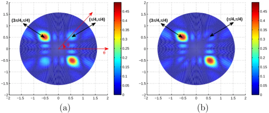
strength of beam pattern in different (φ, θ) is also displayed in the cylindrical coordinate. It can be seen from the figure that there exists a strong mainlobe in the desired direction

of (φ2, θ2) = (3π/4, π/4). While it also shows a strong sidelobe in (φ, θ) = (7π/4, π/4)

and another two obvious sidelobes in (φ, θ) = (5π/4, π/4) and (φ1, θ1) = (π/4, π/4)

which is also the desired direction of user 1. The sidelobe in (π/4, π/4) results in the SINR degradation of user 1.

On the other hand, the beam pattern for user 2 using the HBF of LCMP is shown in Fig. 6.2(b). Though still presenting a strong sidelobe in (φ, θ) = (7π/4, π/4), the

sidelobe is now much weaker in the desired direction (φ1, θ1) = (π/4, π/4) of user 1,

leading to a better SINR for user 1. Besides, the SINR for user 2 in this case is 23.817 dB, while the corresponding SINR for user 2 in Fig. 6.2(a) is 9.366 dB when using the RF BF. Therefore, both users can benefit from a significant SINR improvement using the HBF of LCMP.

In addition to SINR, directivity is also an important performance measure to char-acterize the effectiveness of beamforming. To reflect the interference due to the multiple

−2 −1.5 −1 −0.5 0 0.5 1 1.5 2 −2 −1.5 −1 −0.5 0 0.5 1 1.5 2 0 0.05 0.1 0.15 0.2 0.25 0.3 0.35 0.4 0.45 (3π/4,π/4) (π/4,π/4) θ φ −2 −1.5 −1 −0.5 0 0.5 1 1.5 2 −2 −1.5 −1 −0.5 0 0.5 1 1.5 2 0 0.05 0.1 0.15 0.2 0.25 0.3 0.35 0.4 0.45 (3π/4,π/4) (π/4,π/4) (a) (b)

Figure 6.2: The beam patterns of user two using the RF beamforming and the HBF of

LCMP, with the desired direction set at (φ2, θ2)=(3π/4, π/4).

access in SDMA, the original definition for directivity in [14] is modified into

Di = 4πSINRi(φi, θi) R_2π 0 R π 2 0 |Hi(φ, θ)|2sin(θ)dθdφ . (6.1)

This new definition for directivity automatically refers to the traditional notion of di-rectivity in the single-user system.

User 1 User 2 user 1 (π/8, π/4) user 2 (π/4, π/4)

(φ, θ) RF MD LCMP Opt.1 RF MD LCMP Opt.1

SINR (dB) 22.79 6.993 6.993 22.84 20.17 18.87 18.87 22.84

Directivity 0.5316 0.1631 0.1631 0.6779 0.4665 0.4365 0.4365 0.4102

PT 42.87 42.87 42.87 33.69 43.23 43.23 43.23 53.68

Table 6.1: The SINRs, directivities and the radiation power of the RF BF and the HBF schemes of MD, LCMP and Opt. 1.

TABLE 6.1 presents the simulation results for the SINR, directivity and the radiation

power of various BF schemes for SDMA when the desired directions are set at (φ1, θ1) =

(π/8, π/4) and (φ2, θ2) = (π/4, π/4). The Opt. 1 refers to the HBF scheme of (5.22)

solved with Algorithm 1 in Section 4.2. The radiation power for each user is evaluated with

−2 −1.5 −1 −0.5 0 0.5 1 1.5 2 −2 −1.5 −1 −0.5 0 0.5 1 1.5 2 0.05 0.1 0.15 0.2 0.25 0.3 0.35 0.4 (π/8,π/4) θ φ −2 −1.5 −1 −0.5 0 0.5 1 1.5 2 −2 −1.5 −1 −0.5 0 0.5 1 1.5 2 0.05 0.1 0.15 0.2 0.25 0.3 0.35 0.4 0.45 0.5 (π/8,π/4) (a) (b)

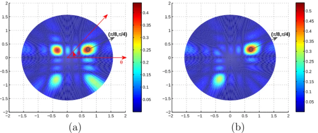
Figure 6.3: The beam patterns of user 1 using the RF BF and the HFB of (5.22), with

the desired direction in (φ1, θ1)=(π/8, π/4).

−2 −1.5 −1 −0.5 0 0.5 1 1.5 2 −2 −1.5 −1 −0.5 0 0.5 1 1.5 2 0 0.05 0.1 0.15 0.2 0.25 0.3 0.35 0.4 0.45 0.5 (π/4,π/4)

Figure 6.4: The beam pattern of user 2 using the HFB of (5.22), with the desired direction in (φ2, θ2)=(π/4, π/4).

and is denoted by PT in the figure.

In this case, even thought RF BF presents similar SINRs of the HBF of Opt. 1, the directivitiy for user 1 of Opt. 1 is much higher than that of the RF BF. However, the directivity for user 2 of Opt. 1 is lower than that of the RF BF. This phenomenon on directivity can be interpreted by users’ beam patterns in Fig. 6.3 ∼ Fig. 6.4.

The beam pattern of user 1 when using the RF BF is presented in Fig. 6.3(a). On the other hand, the beam pattern of user 1 when using the HBF of (5.22) is shown in Fig. 6.3(b). Obviously, there are a strong sidelobe and other two weak ones in addition to the mainlobe in Fig. 6.3(a). However, there only exists a weak sidelobe in Fig. 6.3(b). This indicates that the power for user 1 is more concentrated to its desired direction

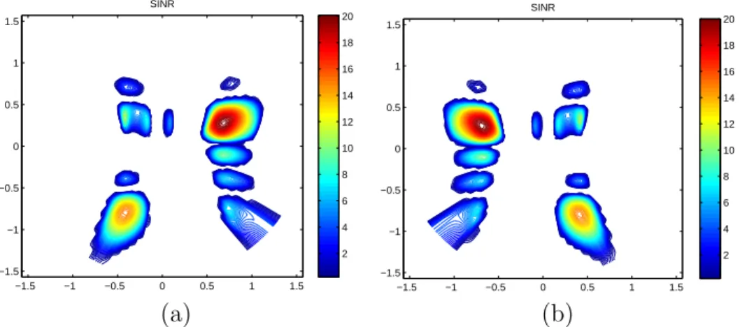
SINR −1.5 −1 −0.5 0 0.5 1 1.5 −1.5 −1 −0.5 0 0.5 1 1.5 2 4 6 8 10 12 14 16 18 20 SINR −1.5 −1 −0.5 0 0.5 1 1.5 −1.5 −1 −0.5 0 0.5 1 1.5 2 4 6 8 10 12 14 16 18 20 (a) (b)

Figure 6.5: The contour plots of SINR for user 1 and user 2 when using the

HBF without the uncertainties, with the desired directions at (φ1, θ1)=(π/8, π/4) and

(φ2, θ2)=(7π/8, π/4), respectively.

with the HBF of (5.22), thus leading to a very high directivity for user 1 in TABLE 6.1. The corresponding beam pattern of user 2 when using the HBF of (5.22) is also shown in Fig. 6.4. In comparison with that of user 1 in Fig. 6.3(b), user 2 has an obvious sidelobe in (φ, θ) = (5π/4, π/4), thus offering a lower directivity than user 1. Besides, directivities of user 2 with Opt.1 are lower than those of the RF BF. Actually, TABLE 6.1 shows that the radiation power of user 2 with Opt.1 is higher than that of the RF BF, and the SINRs of them are close. It means that user 2 must apply more radiation power to achieve the similar SINR of RF BF.

6.2

Robust beamforming for HBF

We demonstrate the simulation results for the HBF with the finite resolution of the phase shifters and robust beamforming methods used to compensate the phase uncer-tainties. Then, comparing the performance of the different robust beamforming scheme. To set K = 4 and L = 8, so there are thirty-two types of the directions applied to the

SINR −1.5 −1 −0.5 0 0.5 1 1.5 −1.5 −1 −0.5 0 0.5 1 1.5 2 4 6 8 10 12 14 16 18 SINR −1.5 −1 −0.5 0 0.5 1 1.5 −1.5 −1 −0.5 0 0.5 1 1.5 2 4 6 8 10 12 14 16 18 20 22 (a) (b)

Figure 6.6: The contour plots of SINR for user 1 when using the exhausting method and simplest method to determine the phase for the HBF with the finite resolution case,

with the desired direction at (φ1, θ1)=(π/8, π/4).

π/180, and the random uncertainties of each patch antenna for the simulation are set

to the uniform distribution U(−5π/180, 5π/180). The desired SINR threshold is set to

20 dB. The desired directions of user one and two are set at (φ1, θ1)=(π/8, π/4) and

(φ2, θ2)=(7π/8, π/4), respectively.

Fig. 6.5 show the contour plots of SINR for user 1 and user 2 when using the HBF without the uncertainties. It achieves the SINR 20 dB at the desired direction of each user by using the total transmit power about 29.25.

Fig. 6.6(a) presents the contour plot of SINR for user 1 when using the exhausting method to determine the phase for the HBF with the finite resolution case. Fig. 6.6(b) presents the contour plot of SINR for user 1 when using the simplest method to determine the phase for the HBF with the finite resolution case. It achieves the desired SINR constraint for each user by using the total transmit power about 35.31. We can find out that the simulation results have some difference between the exhausting method and the simplest method.

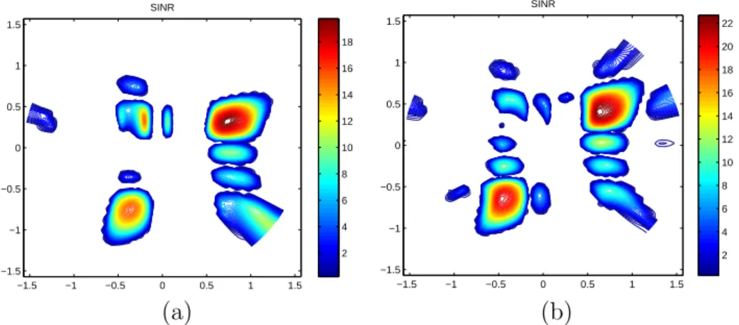
Fig. 6.7(a) presents the contour plot of SINR for user 1 when using the Algorithm 2 for the HBF with the uncertainties. The total transmit power increases to about 70.73 to satisfy the robust condition, and the gray region in this figure shows the SINR above

SINR −1.5 −1 −0.5 0 0.5 1 1.5 −1.5 −1 −0.5 0 0.5 1 1.5 2 4 6 8 10 12 14 16 18 20 (π/8,π/4) SINR −1.5 −1 −0.5 0 0.5 1 1.5 −1.5 −1 −0.5 0 0.5 1 1.5 2 4 6 8 10 12 14 16 18 20 22 (π/8,π/4) (a) (b)

Figure 6.7: The contour plots of SINR for user 1 when using the simplest method to determine the phase for the HBF and using Algorithm 2 and the boundary approach to

compensate the uncertainties, with the desired direction at (φ1, θ1)=(π/8, π/4).

20 dB. Therefore, the SINR at the desired direction of user 1 increases to around 20.64 dB.

Fig. 6.7(b) presents the contour plot of SINR for user 1 when using the boundary approach for the HBF with the uncertainties, and the boundary for two norm of the

steering vector ε is set to √340πδ which can be derived through the definition of δ(n,m)

in (8.7), and δ = ε/6 is the upper bound for ∆ϕi and ∆ϑi, means | ∆ϕi| ≤ δ and

| ∆ϑi| ≤ δ. The total transmit power increases to about 96.28 to satisfy the robust

condition, and the gray region in this figure shows the SINR above 20 dB. Therefore, the SINR at the desired direction of user 1 increases to around 21.63 dB.

TABLE 6.2 shows the performance of various HBF schemes for the different val-ues for the largest phase uncertainty using the simplest method while fixing the SINR threshold as 20 dB. We can find out that the larger boundary ² needs more total power to achieve the fixed SINR constraints. TABLE 6.3 presents the performance with various HBF schemes for the different values of the largest phase uncertainty using the simplest method for the same total power constraint. It demonstrates that the achievable SINR for each user for different robust methods with the total power constrained as 60 dB.

User 1 (π/8, π/4) Ideal (user 1) Algorithm 2 (user 1) Boundary (user 1)

User 2 (7π/8, π/4) PT SINR (dB) PT SINR (dB) PT SINR (dB)

² = 0 29.65 20 − − − − ² = π/180 , δ = ²/6 − − 70.73 20.64 96.28 21.63

² = 2π/180 , δ = ²/6 − − 82.02 21.44 153.09 23.61

² = 3π/180 , δ = ²/6 − − 98.79 22.42 277.26 26.14 Table 6.2: The table of the performance with various HBF schemes for the different values of the largest phase uncertainty using the simplest method for the same SINR constraint.

User1(π/8, π/4) Ideal (PT = 60) Algorithm 2 (PT = 60) Boundary (PT = 60)

User2(7π/8, π/4) SINR1 SINR2 γ0 SINR1 SINR2 γ0 SINR1 SINR2 γ0

² = 0 22.97 22.97 22.97 − − − − − − ² = π/180 , δ = ²/6 − − − 19.98 19.63 19.35 19.64 19.60 18

² = 2π/180 , δ = ²/6 − − − 20.17 19.41 18.75 19.63 19.57 16

² = 3π/180 , δ = ²/6 − − − 20.37 19.12 18 19.64 19.57 13.45 Table 6.3: The table of the performance with various HBF schemes for the different

values of the largest phase uncertainty using the simplest method for the same total power constraint.

Chapter 7

Conclusions

We investigated hybrid beamforming for SDMA in 60GHz applications using PAA. According to different transmit requirements, different design criteria can be applied based on the convex optimization. For the practical applications, we consider the finite resolution problem about the RF beamforming and the phase uncertainties. The robust beamforming can be applied to compensate the phase uncertainties. Therefore, we can jointly design the phases and weights based on the convex optimization to guarantee the SINR of each user. We demonstrate that the hybrid beamforming scheme for SDMA is feasible and is a promising technique.