應用於查找表式場域可程式化閘陣列之壓縮樹延遲最佳化合成演算法

國立交通大學

電子工程學系 電子研究所碩士班

碩 士 論 文

應用於查找表式場域可程式化閘陣列之壓縮樹

延遲最佳化合成演算法

Delay Optimal Compressor Tree Synthesis for

LUT-Based FPGAs

研 究 生：呂智宏

指導教授：周景揚 博士

黃俊達 博士

應用於查找表式場域可程式化閘陣列之壓縮樹延遲最

佳化合成演算法

Delay Optimal Compressor Tree Synthesis for

LUT-Based FPGAs

研 究 生：呂智宏

Student: Jhig-Hong Lu

指導教授：周景揚 博士

Advisor: Dr. Jing-Yang Jou

黃俊達 博士

Advisor: Dr. Juinn-Dar Huang

國 立 交 通 大 學

電子工程學系電子研究所碩士班

碩 士 論 文

A Thesis

Submitted to Department of Electronics Engineering & Institute of Electronics College of Electrical and Computer Engineering

National Chiao Tung University in Partial Fulfillment of the Requirements

for the Degree of Master

in

Electronics Engineering July 2009

應用於查找表式場域可程式化閘陣列之壓縮樹

延遲最佳化合成演算法

摘要

Delay Optimal Compressor Tree Synthesis

for LUT-Based FPGAs

Student: Jhih-Hong Lu

Advisor: Dr. Jing-Yang Jou, Dr. Juinn-Dar Huang

Department of Electronics Engineering Institute of Electronics

National Chiao Tung University

Abstract

In this thesis, we present a compressor tree synthesis algorithm, named DOCT,

which guarantees the delay optimal implementation in lookup-table (LUT) based

FPGAs. Given a targeted K-input LUT architecture, DOCT firstly derives a finite

set of prime patterns as essential building blocks. Then, it shows that a delay

optimal compressor tree can always be constructed by thosederived prime patterns

via integer linear programming (ILP). Without loss of delay optimality, a

post-processing procedure is invoked to reduce the number of demanded LUTs for

the generated compressor tree design. DOCT has been evaluated over a broad set of

benchmarkcircuits. Compared to the previous heuristic approach, the experimental

results show that DOCT reduces the depth of the compressor tree by 32%, and the

Acknowledgment

At first, I deeply appreciate my advisor Professor Jing-Yang Jou. Not only did

he made many beneficial suggestions for me, but also provide a resource-intensive

environment. I am also really thankful to my co-guidance advisor Professor

Juinn-Dar Huang for his guidance. He is a constant inspiration to me. I would like

to thank Bu-Ching Lin and Wan-Hsien Lin. Without their support, I could not finish

my research. Thanks to Yu-Shiang Wang, Ji-Huei Li, and Wan-Ling Shiu, for their

friendship and encouragement. And thanks to all members of EDA laboratory. During the past two years, each one of them was never afraid to offer their opinions. This kind of favor enlivened my train of thought in my academic field. Finally and especially, I would like to express my sincere acknowledgement to my family and all my friends for their aid.

Content

Abstract ... iv

Acknowledgment ... v

Content ... vi

List of Tables ... viii

List of Figures ... ix Chapter 1 Introduction ... 1 1.1 Technology Trend ... 1 1.2 Previous Works ... 1 1.3 Contribution ... 3 1.4 Thesis Organization ... 3 Chapter 2 Preliminaries... 4 2.1 Compressor Trees... 4 2.2 Definitions... 5 2.3 Problem Formulation ... 8

2.4 Properties of Prime Patterns... 11

Chapter 3 Proposed Algorithm... 17

3.1 Upper Bound Determination ... 18

3.2 Variables ... 20

3.3 Covering and Succeeding Constraints ... 21

3.4 Column and Stratum Constraints ... 22

3.5 Objective Function ... 24

Chapter 4 Experiments ... 29 4.1 Experimental Information ... 29 4.2 Parameters Setup ... 30 4.3 Experimental Results ... 31 Chapter 5 Conclusions ... 34 Reference ... 35

List of Tables

TABLE I CIRCUIT INFORMATION ... 30

TABLE II SYNTHESIS RESULTUNDER K = 5 ... 31

TABLE III SYNTHESIS RESULTUNDER K = 6 ... 32

List of Figures

Figure 2.1 An example of a compressor tree on ASICs. ... 4

Figure 2.2 The expression of a odt plane and a pattern. ... 5

Figure 2.3 (a) PPS(1) (b) PPS(2) (c) PPS(3) ... 6

Figure 2.4 Matches under the dot plane d₀ 3, 4, 2 ... 9

Figure 2.5 Illustrations for coversunderthe dot plane d₀ 3, 4, 2 ... 10

Figure 2.6 General compressor tree synthesis pseudo code. ... 11

Figure 2.7 All subpatterns of the pattern p41, 2p ... 11

Figure 2.8 Illustration for decompose( 3,1, 0,1 p). ... 12

Figure 3.1 DOCT flow. ... 17

Figure 3.2 Examples of a extension and cover ... 18

Figure 3.3 Examples of compressor tree synthesis ... 20

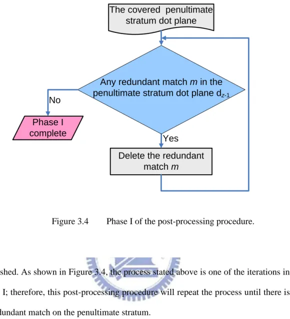
Figure 3.4 Phase I of the post-processing procedure ... 25

Figure 3.5 A two-output LUT with shared inputs. ... 26

Chapter 1

Introduction

1.1

Technology Trend

As the manufacturing cost and time-to-market pressure of developing

ASIC/SoC increase, the design and verification processes demand a better way to

reduce the development cost. The advantages of low risk, low NRE cost, and fast

time-to-market, have made FPGA a significant alternative for the electronic system

design, and then FPGA is usually used for flexible and low-volume applications

without regard to system performance. However, a high-performance system can be

possibly implemented with modern FPGAs, since an FPGA device can have a very

rich set of logic elements and very high-speed I/O interfaces under recent DSM

technologies [1-4]. The arithmetic circuit, rather than the control-dominated circuit,

is often the performance bottleneck for a high-performance system implemented

with FPGAs [5, 6] and thus this thesis presents an algorithm for the delay optimal

compressor tree synthesis.

1.2

Previous Works

A compressor tree is used to implement a multi-operand addition, which is one

of the essential operations in most DSP applications, e.g., FIR/IIR filters [7],

compressor tree has been introduced by Wallace and Dadda for more than 40 years

[10, 11]. An efficient method, called Three-Greedy Approach, is proposed in [12]

for the delay-optimized compressor tree synthesis. A delay optimal algorithm

without considering wire delay is further presented in [13]. All the building blocks

for the above two researches are restricted to full-adders and half-adders. However,

since the basic programmable logic block in a modern FPGA is a K-input LUT

(K 5 or 6), 3-input full-adders and 2-input half-adders are apparently not the appropriate building blocks for compressor tree synthesis from both area and delay

perspectives.

Algorithms proposed in [14] and [15] have made significant progresses in

reducing the delay of the compressor tree in FPGA designs. Although the GPC

heuristic has achieved reasonably good results [14], its inherently heuristic nature

cannot guarantee optimal solutions. Moreover, an algorithm which utilizes a set of

GPC patterns is presented in [15] for the delay-optimized compressor tree

construction via integer linear programming (ILP). However, this method does not

consider all valid GPC patterns under a given input constraint (i.e., K); therefore, it

cannot guarantee optimal solutions, either. According to [15], the compressor trees

synthesized by the above two algorithms even have the same depth in many cases.

A hybrid architecture is presented to obtain advantages of both ASIC and

FPGA technologies [16]. ASICs offer advantages of density and performance. On

the other hand, FPGAs offer advantages of flexibility and fast time-to-market. By

the same manner, hard configurable IP cores are developed to integrate into FPGAs

for accelerating the speed of compressor trees [17, 18]. But this kind of approaches

1.3

Contribution

In this thesis, we present a delay optimal compressor tree synthesis algorithm,

named DOCT, for LUT-based FPGAs. It firstly derives a set of prime patterns as

essential building blocks, and then utilizes them to construct the delay optimal

compressor tree via ILP. Besides, a post-processing procedure is invoked to

minimize the number of demanded LUTs without loss of delay optimality.

Compared to the GPC heuristic [14], the experimental results show that DOCT

reduces the depth of the compressor tree by 32% and the number of LUTs by 21%

on average based on the modern 6-input LUT-based FPGA architecture.

1.4

Thesis Organization

The rest of this thesis is organized as follows. Terminology, definitions,

fundamental theorems, and problem formulation are introduced in Chapter 2.

Chapter 3 details the proposed delay optimal compressor tree synthesis algorithm

with ILP formulation. The experimental results are then presented in Chapter 4.

Chapter 2

Preliminaries

2.1

Compressor Trees

A compressor tree is a circuit dealing with a multi-operand addition. Before

1960s, the multi-operand addition was often accumulated by the carry-propagate

adder (CPA). To minimize the delay of the carry chain produced by several CPAs,

Wallace and Dadda proposed an efficient implementation in 1960s to reduce all

partial products into two partial products by full-adders and half-adders, and to add

the final two partial products by a CPA. Three reduction rules are used for

constructing compressor trees: (i) any three dots with the same rank can be mapped

onto a full adder, (ii) the remaining two dots with the same rank can be mapped

onto a half adder or passed to the next stratum, and (iii) the last dots are directly

passed to the next stratum. The full adder acts as a 3:2 counter to add as many dots

as possible with the same rank. Figure 2.1 shows an example of a compressor tree

half adder full adder 0







on ASICs, which reduces three partial products into two partial products.

2.2

Definitions

Firstly, this subsection describes a formal expression to characterize the

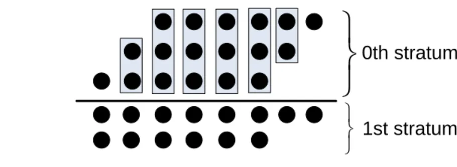
topology of the compressor tree. A compressor tree consists of a series of strata.

Each stratum is represented by a dot plane. A dot plane with respect to the s-th

stratum is denoted as an n-tuple 2 1, 2,..., 0

n s n n

d t _ t_ t ZN  Z, where N is the set of non-negative integers, Z+ is the set of positive integers, and ti indicates the

number of dots which is in the i-th column of the dot plane on the s-th stratum of

the compressor tree. The set of dot planes is defined as D, and then the function

column: 2 1 0 _{column: 1 0}











(a)

(b)

(c)

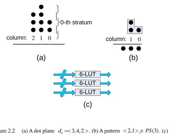
Figure 2.2 (a) A dot plane d₀ 3, 4, 2. (b) A pattern 2,1 _p PS(3). (c) The pattern 2,1_p is mapped onto 3 6-input LUTs.

:

r D N N can indicate the i-th element of the dot plane d_s by r d i( , )_s t_i. The function w D: Z defines the width of each dot planesuch that w d( )s n

iff d is an n-tuple; meanwhile, the function _s h D: Z defines the height of the dot plane d according to_s h d( )_s max{ ( , ) | 0r d i_s  i w d( )}_s . Figure 2.2(a) provides an illustrative example as follows. The dot plane d03, 4, 2 is the

input of a compressor tree consisting of three columns: two dots in the 0th column,

four dots in the 1st column, and three dots in the 2nd column. Therefore, the height

and the width of the dot plane d0 are h d( 0)max{3, 4, 2}4 and w d( 0)3,

respectively.

The following subsection describes a formal expression to characterize the

pattern. A pattern is denoted as an m-tuple 2 1, 2,..., 0

m m m p

p t _ t _ t  ZN  Z,

where tj indicates the number of dots which is in the j-th column of the pattern p.

The set of patterns is denoted as P, and then the function v P N:  N can indicate the j-th element of the pattern p by v p j( , )tj . The function

:

iw PZ defines the number of input columns of each pattern, i.e., iw p( )m

iff pt_m1,t_m2,...,t₀_p. All patterns have the corresponding number of their

(a)

(b)

(c)

p

p

p

p

output bits. Thus the function ow P: Z calculates the minimal number of the required output bits by ( ) 1

0 2

( ) log ( iw p ( , ) 2 )i i

ow p    v p i  . A pattern is similar to a

counter in functionality, but it can sum inputs with value 1 in different ranks. For

example, a 3:2 counter like p3 as shown in Figure 2.3(c) sums three rank-0 inputs

while the pattern 2,1_p as shown in Figure 2.2(b) sums two rank-1 inputs and one rank-0 input. Furthermore, the number of input columns of the pattern

2,1 p

  is iw( 2,1  p) 2, and the number of its output bits is ow( 2,1  p) 3.

The function PS: Z P( )P points out the power set of patterns such that ( ) pPS k iff ( ) 1 0 ( , ) iw p i v p i k   

 , e.g., a pattern p belongs to PS(3), which implies i ( )-1

0 ( , ) 3

w p

i v p i 

 . Moreover, the function UPS: Z P( )P points out a union of pattern sets such that ( ) 1 ( )

k i

UPS k  PS i .

Since a single LUT in the FPGA has the input constraint K (K6 for modern technologies), a pattern pUPS K( ) can be mapped onto ow p( ) copies of the

K-input LUT. For example, the pattern 2,1_p can be mapped onto 3 copies of the 6-input LUT as shown in Figure 2.2(c). The delay is obviously equal to a LUT

delay as all patterns belong to UPS K . The delay optimal compress tree can be ( )

constructed with UPS K , but ( ) UPS K is an infinite set. In other words, we ( )

cannot determine the optimal solution with UPS K unless there is a finite set to ( )

construct the compressor tree without loss of delay optimality.

This thesis shows that a finite subset of the infinite set UPS K does exist to ( )

construct the compressor tree without loss of delay optimality. We denote the finite

set as PP and take patterns in it as prime patterns. Therefore, pPP iff

1 _p (1)

p  PS , or p has the property -1

0 ( , ) 2 2

i j j

i v p i  

the carry propagation in each of its columns. For example, the prime pattern

4 1, 2 p

p   as shown in Figure 2.3(c) possibly produces two valid carries in the 0th and 1st columns due to 0 1

4 ( , 0) 2 2 v p   and 1 2 0 ( 4, ) 2 2 i i v p i    ,

respectively. On the other hand, the pattern 2,1_p is not a prime pattern because it will never produce a valid carry in the 0th column due to 0 1

( 2,1 p, 0) 2 2

v     .

The function PPS: Z P(PP) points out a power set of prime patterns such that pPPS k( ) iff p{PPPS k( )}. For instance, a pattern p belongs to

(3)

PPS , which implies pPP and ( )-1

0 ( , ) 3

iw p

i v p i 

 , as shown in Figure 2.3(c). Moreover, Figure 2.3 illustrates three sets of prime patterns as follows:

1

(1) { }

PPS  p , PPS(2){p₂} , and PPS(3){p p₃, ₄} . The function

: ( )

UPPS Z P PP points out a union of prime pattern sets such that

1

( ) k ( )

i

UPPS k  PPS i , and the function UNPPS: Z P(PP) points out a set

of non-prime patterns by UNPPS k( )UPS k( )UPPS k( ).

For the modern technology, there are only 37 distinct prime patterns in

(6)

UPPS ; therefore, we can find the delay optimal compressor tree based on

(6)

UPPS . For simplicity, all examples are demonstrated under K3 in the rest of this thesis.

2.3

Problem Formulation

Before formulating the compressor tree problem, this thesis introduces the

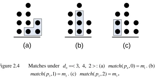
relationship between the dot plane and the pattern. In this thesis, a match is a

subgraph indicating the relationship between a pattern and a collection of dots, and

Figure 2.4 demonstrates three feasible matches under the dot plane d₀ 3, 4, 2:

4 1

( , 0)

match p m , match p( ₃,1)m₂, and match p( ₂, 2)m₃. In other words,

Figure 2.4(b) illustrates that three dots in the 1st column of d0 are matched to the

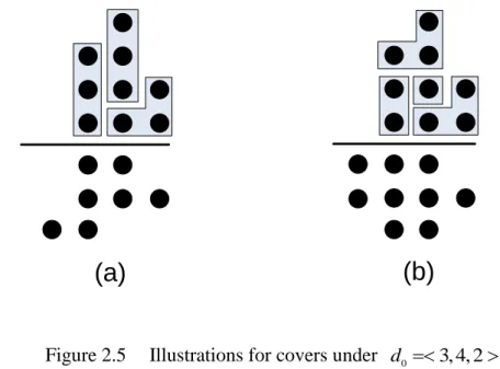
prime pattern p3 by m2. Furthermore, a cover is a set of matches such that each dot

in the same dot plane is matched exactly once by a certain pattern, and then the

mapping is defined as cover: (P M)C, where C is the set of covers. Figure 2.5 demonstrates two feasible covers under the dot plane d₀ 3, 4, 2: the cover

1 2 4 1

({ , , })

cover m m m c with m4match p( 3, 2) ; the cover

1 3 5 6 2

({ , , , })

cover m m m m c with m₅ match p( ₁,1) _and m₆ match p( ₄,1). Since the dot plane d_s1 depends on the cover under the dot plane d , we can _s

express ds1 by the output derived from the cover under d . Therefore, the s

function map: D C D determines the resultant dot plane d_s1 after the dot

plane d is covered by the specific cover. For instance, Figure 2.5 shows two s

resultant dot planes, map d c( ₀, )₁ 1,3, 2,1 and map d c( ₀, ₂)2,3,3,1 , derived from covers c₁ and c₂ under the dot plane d₀3, 4, 2, respectively.

(a)

(b)

(c)

Figure 2.4 Matches under d₀ 3, 4, 2: (a) match p( ₄, 0)m₁. (b)

3 2

( ,1)

On modern FPGAs, a ternary adder can sum three operands simultaneously. For

flexibility, we denote the maximum quantity of operands as H for a CPA on the

targeted FPGA. Therefore, H is equal to 3 in modern FPGAs. In the future, H may

be increased to 4, 5, 6, and so on; therefore, we can construct the compressor tree

by executing a sequence of covers until the height of the dot plane is less than or

equal to H. After the compressor tree is constructed completely by the sequence of

covers, at most H numbers are summed by a CPA. Since the delay of a pattern in

( )

UPS K is equal to a LUT delay, the depth of the compressor is equal to the times

of executing covers. Apparently, the fewer the times of executing covers is, the less

the depth of the compressor tree is. This thesis describes a general pseudo code to

construct compressor trees, as shown in Figure 2.6. Before we execute the loop

body, the height of the dot plane will be checked whether it is larger than H. If the condition is true, the dot plane needs a specific cover to reduce its height. After the

dot plane d is covered by the cover c_s s, the resultant dot plane ds1, will be

produced by map d c( s, s). Therefore, the depth of the compressor tree is equal to

the times of executing loop. The unit delay model is used such that the delay is

(a)

(b)

determined by the depth of the compressor tree. Thus, we can declare that a

compressor tree is delay optimal if its depth is the minimum.

2.4

Properties of Prime Patterns

In order to synthesize the delay optimal compressor tree, the set of building

blocks should contain patterns where the number of inputs (i.e., i ( )-1 0 ( , )

w p

i v p i

 ) is equal to or less than K. In other words, the set of building blocks will be UPS K( )

exactly. Since UPS K( ) is an infinite pattern set, considering all combinations of

the compressor tree with UPS K( ) is impossible. This thesis describes the truth

(a)

(b)

(c)

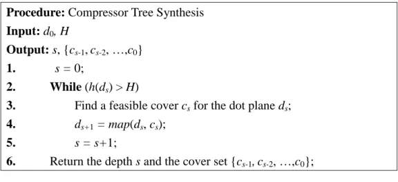
Procedure: Compressor Tree Synthesis Input: d0, H

Output: s, {cs-1,cs-2, …,c0}

1. s = 0;

2. While (h(ds) > H)

3. Find a feasible cover cs for the dot plane ds;

4. ds+1 = map(ds, cs);

5. s = s+1;

6. Return the depth s and the cover set {cs-1,cs-2, …,c0};

that the delay optimal compressor tree can be constructed by the finite set

( )

UPPS K , rather than UPS K( ), without loss of delay optimality.

Before describing the fundamental theorem, we define the subpattern firstly.

The function sub N:   N P P defines the subpattern ( , , ) ( , ), ( , 1),..., ( , ) p

sub j i p v p j v p j v p i  P with the constraint

0  i j iw p( ). Figure 2.7 shows all subpatterns of the pattern p₄ 1, 2p:

4

(1,1, ) 1 p

sub p   , sub(0, 0,p₄) 2 p , and sub(1, 0,p4)1, 2p . In the following, this thesis defines pattern decomposition. The function

: ( )

decompose PP M defines a list of feasible matches {(sub j i p k( , , ), )} such

that the following conditions can be satisfied: (i) ( , )x i decompose p( ) :xPP,

and (ii) 2

(( , ), ( , ))x i y j decompose p( ) , i j ow y: ( ) j 1 i

      . Figure 2.8

shows that the pattern 3,1, 0,1p can be partitioned into { ,p p p because of 1 1, 3}

the pattern decomposition decompose( 3,1, 0,1  p) {(p₁, 0), (p₁, 2), (p₃, 3)} .

Then, this thesis shows that all patterns can be partitioned into a set of prime

patterns.

decompose

Lemma 1: For each pattern pUPS k( ), p can be partitioned into a set of prime patterns Ep { | ( , )pˆ p iˆ decompose p( )}.

Proof: In the beginning, we identify whether p belongs to UPPS(k). If

( )

pUPPS k , E_p  p. Otherwise, we check the carry propagation possibility from the 0th column to (iw(p)−1)-th column in the pattern p. Because p belongs to

UNPPS(K), there exists a set of non-negative integers





0

| 0 ( ) and q ( , ) 2i 2q i

p

Q  q  q iw p  v p i    ; otherwise, p should belong to

( )

UPPS K , which contradicts pUNPPS k( ). Based on qmin{Q_p}, let the pattern ˆp be the identified pattern with the property ₀ iw p(ˆ₀) q 1 such that

0

ˆ

( , ) ( , )

v p i v p i for 0 i iw p(ˆ₀) and ( , )v p j 0 for iw p(ˆ₀) j q. Due to

min{ _p}

q Q , ˆp is a prime subpattern of p. Similarly, let '₀ p be the subpattern

of p with the property iw p( ')iw p( )q such that ( ', ) ( , ( ) ( ') )

v p i v p iw p iw p i for 0 i iw p( ') , and v p j( , )0 for ( ) ( ')

q j iw p iw p . Obviously, p'sub iw p( ( ) 1, iw p( )iw p( '), )p UPS k( ) is true. If p is prime, ' p can be partitioned into Ep {p pˆ0, '}; therefore, this

lemma holds true. The above process, called cut, can extract another prime

subpattern on p . After we repeat cuts on ' p , p can be partitioned into '

0 1

ˆ ˆ ˆ { , ,..., }

p

E  p p p_ such that ˆp is a prime pattern for 0 ii   . Since p belongs

to UPS k , all patterns in ( ) E do belong to p UPPS k . Moreover, ( ) Ep is surely finite since each cut extracts a pattern ˆp under i iw p( ) 1ˆi  . In other words, the

p can be partitioned into a set of prime patterns Ep { | ( , )pˆ p iˆ decompose p( )}.

According to Lemma 1, it is obvious that a non-prime pattern can be replaced

by a set of prime patterns. Therefore, Lemma 2 can be deduced by Lemma 1. Due

to pattern decomposition, the output of a non-prime pattern p may be different to

that of Ep. For example, the pattern 3,1, 0,1p has the output 1,1,1,1,1, but its decomposition decompose( 3,1, 0,1  p) {(p₁, 0), (p₁, 2), (p₃, 3)} has the

output 1,1,1, 0,1, as shown in Figure 2.8(b). The new cover ˆc is derived after

every non-prime pattern p is partitioned into E_p, where match p i( , )c, c is a feasible cover under the dot plane d , and _s 0 i w d( _s). Thus, map d c never ( , )_s ˆ produces more dots than map d c does. In the following, Lemma 2 shows that a ( , )s

compressor tree constructed with non-prime patterns can be replaced by a

compressor tree constructed with prime patterns, and then the latter has the same or

less depth.

Lemma 2: If there exists a compressor tree T constructed with UPS k( ), there exists

another compressor tree T' constructed with UPPS k such that the depth of ( ) T'

is equal to or less than that of T.

Proof: Let T be a compressor tree constructed with UPS k and the depth of T be ( )

z. The cover c is assumed to be under the dot plane s d on the s-th stratum of T s

for 0 s z . According to Lemma 1, a non-prime pattern

0

{ ' | : ( ', ) and ' ( )}

p p a match p a c p UNPPS k could be partitioned into a set of prime patterns E_p UPPS k( ). After pattern decomposition, the new cover is

denoted as ˆc and 0 map d c is denoted as ( 0, )ˆ0 ˆd . Since the decomposition may 1

delete some dots of d , i.e., ₁ r d a( , )ˆ₁ r d a( , )₁  a for 0 a w d( )ˆ1 , where

0

a

  . Thus, there is a new cover c under ₁' ˆd such that a non-empty set of dots ₁ '

Q in ˆd is matched by a certain match 1 m'c1' iff Q'Q, Q and Q are '

maximal, and Q is matched by a certain match mc1. In the same way, a

non-prime pattern p{ ' |p match p b( ', )c₁ and 'p UNPPS k( )} can be partitioned into a set of prime patterns E_p UPPS k( ) . After pattern decomposition, the new cover is denoted as ˆc , and then the dot plane 1

2 1 1

ˆ _{( , )ˆ ˆ}

d map d c is derived such that w d( )ˆ₂ w d( )₂ and r d b( , )ˆ₂ r d b( , )₂  b

for 0 b w d(ˆ₂), where  b 0. This thesis calls the above process as transfer.

By executing transfers from d to 3 dz1, we can partition each non-prime pattern

in T into a set of prime patterns. In the end, there are two cases of ˆc for _s

0 s z: (i) each dot in ˆd is match to _s p1  1 p , and (ii) ˆc contains at least s

one match match p i( , ), where 0 i w d( )ˆ_s and p 1 _p. If ˆc belongs to _s

Case (i), ˆc makes no delay; otherwise, ˆ_s c has a LUT delay. Therefore, T could s

be transferred recursively into T' with the depth z' such that z'z.

By Lemma 2, we acknowledge that every compressor tree containing

non-prime patterns can be transformed into the compressor tree which only

contains prime patterns. In the following, this thesis deduces the key theorem by

Theorem 1: The minimum depth of compressor tree constructed with UPS k is ( )

the same as that of the compressor tree constructed with UPPS k . ( )

Proof: Let T be the compressor tree constructed with UPS k( ), and T' be the

compressor tree constructed with UPPS k( ); meanwhile, T and T' have the

minimum depth z and z’. Since UPS k contains ( ) UPPS k( ), i.e., the solution

space with UPPS k is the subset of that with ( ) UPS k , we can derive that ( )

'

z z. According to Lemma 2, a compressor tree constructed with UPPS k( ) has the depth z"z. Since T' is the compressor tree constructed with UPPS k( )to have the minimum depth, we can derive that z'z"z. Due to z'z and

'

z z, z is equal to z'.

According to the theorem, the delay optimal compressor can be constructed

with UPPS K , rather than ( ) UPS K . In other words, ( ) UPPS K is a compact ( )

set of basic building blocks for compressor trees. Throughout the rest of this thesis

Chapter 3

Proposed Algorithm

In this chapter, this thesis describes a delay optimal compressor tree synthesis

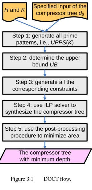
algorithm, DOCT, to synthesis compressor trees. The detail processes are shown in

Figure 3.1. Step 1 generates all prime patterns in UPPS K . Step 2 determines the ( )

upper bound of the minimum depth, denoted as UB, under the given input of the

compressor tree. Under UB, Step 3 unrolls the loop as shown in Figure 2.6 to

Specified input of the compressor tree d0

H and K

Step 1: generate all prime patterns, i.e., UPPS(K)

Step 2: determine the upper bound UB

Step 3: generate all the corresponding constraints

Step 4: use ILP solver to synthesize the compressor tree

Step 5: use the post-processing procedure to minimize area

The compressor tree with minimum depth

generate all the corresponding constraints and the objective function. Step 4 gains

the delay optimal compressor tree via the ILP solver. Furthermore, Step 5 uses a

post-processing procedure to minimize area overhead.

3.1

Upper Bound Determination

Since this thesis unrolls the loop as shown in Figure 2.6 to get the delay

optimal compressor tree, the upper bound of the minimum depth needs to be

determined in advance. Therefore, this subsection describes how to determine UB.

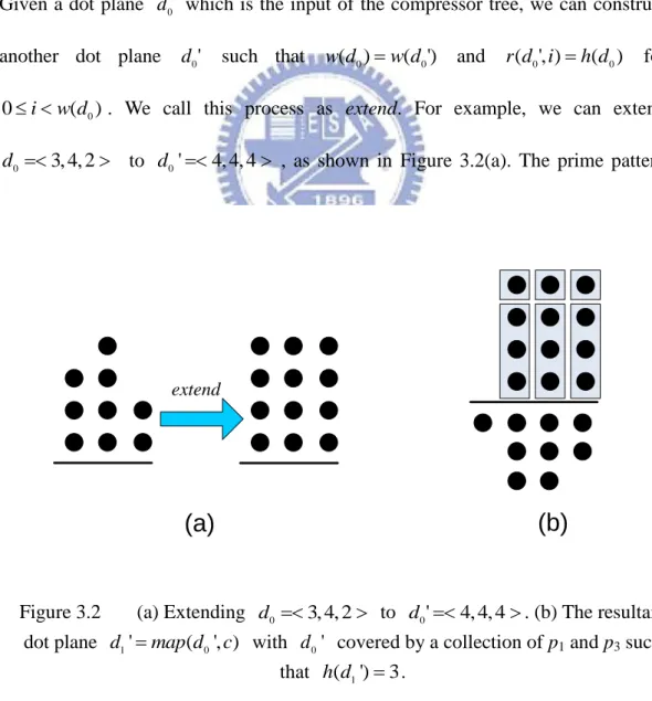
Given a dot plane d which is the input of the compressor tree, we can construct ₀

another dot plane d₀' such that w d( ₀)w d( ')₀ and r d i( ', )₀ h d( ₀) for

0

0 i w d( ). We call this process as extend. For example, we can extend

0 3, 4, 2

d   to d₀'4, 4, 4 , as shown in Figure 3.2(a). The prime pattern

extend

(a)

(b)

Figure 3.2 (a) Extending d₀ 3, 4, 2 to d₀'4, 4, 4. (b) The resultant dot plane d₁'map d( ₀', )c with d covered by a collection of p₀' 1 and p3 such

p

xK  matches as many dots in the dot plane d as possible if K is equal to 0'

or less than h d( 0'). Then, the prime pattern yh d( 0') modK p matches the remaining dots, where K is the given input constraint of a LUT. Since d is 0'

regular, we can determine h d( ₁') precisely by the equation (1), where

1' ( 0', )

d map d c is a dot plane derived from the cover



 



0 ( , ) 0 ( , )

w d w d

i j

c   match x i     match y j . Therefore, the upper bound of the

estimation, min{ ( ) |h d₁  c C d: ₁map d( ₀', )}c _{, can be determined by} h d( ₁').

1

( s ') ( s') / ( < > )p ( < ( s') mod > )p

h d h d Kow K ow h d K (1)

In all cases of this thesis we assume H 2. To determine UB, we execute the equation (1) recursively until h d( _s1') is equal to or less than H. As the times of

executing the equation (1) is z', z' and UB should be equal. For example, based

on K3 and d₀'4, 4, 4 , nine dots in d are matched to ₀' p₃ 3 _p

firstly, and then the others are matched to p₁4 mod 3_p, as shown in Figure 3.2(b). Therefore, we can derive the upper bound of the minimum height of the dot

plane d as ( 4 / 3₁'  ow( 3  p) ow( 4 mod 3 p))3 . Moreover, we can determine the upper bound of the minimum height of the dot plane d as 2 by the 2'

equation (1). Since h d( ₂') is equal to H, the determination process for UB is

terminated. In this example, the times of executing the equation (1) is 2. Hence, UB

3.2

Variables

This subsection introduces the variables used in ILP formulation.

xs,i,j: the count of the match match p i( j, ) occurring on d s hs,i: the number of dots in the i-th column of ds, i.e., ( , )r d i s

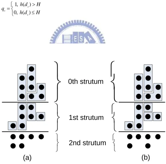
, 1, ( , ) 0, ( , ) s s i s r d i H c r d i H     _  1, ( ) 0, ( ) s s s h d H q h d H     _ 

0th strutum

1st strutum

2nd strutum

(a)

(b)





































Figure 3.3 (a) The compressor tree before area minimization. (b) The compressor tree after Phase I of the post-processing procedure.

Figure 3.3(a) shows that the dot plane d₀ 3, 4, 2 has a cover

0 ({ 1, 2, 3})

c cover m m m which is constructed from m1match p( 4 1, 2p, 0) ,

2 ( 3 3 p,1)

m match p   , and m₃match p( ₃, 2)_{; therefore,} x0,0,4 x0,1,3 x0,2,3 1

and other variables x0, ,i j on the 0th stratum are equal to zero. Furthermore, the dot plane d₁1,3, 2,1 has a cover c₁cover m m m m({ ₃, ₄, ₅, ₆}) which is constructed from m₄match p( ₁ 1 p, 0), m5match p( 2  2 p,1), and m6 match p( 1, 3);

therefore, x1,0,1x1,1,2 x1,2,3 x1,3,1 1, and other variables x1, ,i j on the 1st stratum are equal to zero.

3.3

Covering and Succeeding Constraints

The constraint (2) is called as covering constraint used to enforce a feasible

cover under the dot plane ds. We use the covering constraint to ensure that every dot

is matched exactly once. The inner summation of the constraint (2) sums the

amount of dots in the i-th column of ds, and they are matched to the prime pattern pj

by the match match p i( j, k) for 0 k min{ (iw pj),i1}. Further, the outer summation of the constraint (2) sums all the results of the inner summation for all

prime patterns. Figure 3.3(a) shows that the covering constraint enforces a feasible

cover cover m m m({ 1, 2, 3}) under the dot plane d0 3, 4, 2 such that

0,0,4 0,0

| ( )| ( ) 1 , , , 1 0 ( , ) , 0 ( ), 0 j UPPS K iw p j s i k j s i s j k v p k x h i w d s UB            





Since the dot plane ds+1 depends on how the preceding dot plane ds is covered,

we need the constraint (3) to construct the dot plane ds+1 such that hs1,i r d( s1, )i

for 0 i w d( _s1). This thesis calls the constraint (3) as succeeding constraint. Firstly, the inner summation of the constraint (3) sums the number of matches

( j, )

match p ik for 0 k min{ow p( _j),i1} to get the dots in the i-th column of the dot plane ds+1; meanwhile, the dots are contributed by the pattern pj. Further, the outer summation of the constraint (3) sums all the results of the inner

summation for all prime patterns to get hs+1,i. Figure 3.3(a) shows h1,0 x0,0,4 1,

1,1 0,1,3 0,0,4 2

h x x  , h_1,2 x_0,1,3x_0,2,3x_0,0,4 3, and h_1,3 x_0,2,31, where the dot planed₀3, 4, 2 has the cover cover({(p₄, 0), (p₃,1), (p₃, 2)}).

| ( )| ( ) 1 , , 1, 1 0 , 0 ( ), 0 j UPPS K ow p s i k j s i s j k x h i w d s UB            





3.4

Column and Stratum Constraints

The union of the constraints (4) and (5) is used to compute the correct cs,i. This

thesis calls the union of the two constraints as column constraint. If the i-th element

1. On the other hand, cs,i will be enforced to be 0 as hs,i is equal to or less than H. In

Figure 3.3(a), due to h_1,12 and h_1,2 3, c1,1 is set as 0 and c1, 2 is set as 1 via the

column constraint. Besides, the term Inf used in the constraints (5) and (7) can be

set as ( 0) 1 0 ( 0, ) w d i r d i    . , , (H  2) c_{s i}  1 h_{s i} , 0  i w d( _s), 0  s UB (4) , ,, 0 ( ), 0 s i s i s Inf c H h   i w d   s UB (5)

When the compressor tree is constructed completely, q_s 0 and h d( )s H

should be satisfied iff the depth is equal to s. Therefore, a CPA can be used.

Otherwise, the dot plane ds still need be covered to reduce its height. This thesis

uses cs,i to obtain qs via the constraints (6) and (7). The union of these two

constraints is called as stratum constraint. Figure 3.3(a) shows an illustrative

example. The variable q1 is set as 1 via the stratum constraint due to h d( )1  3 H.

On the other hand, the variable q2 is set as 0 due to h d( 2) 2 H.

( ) 1 , 0 , 0 s w d s i s i q 





3.5

Objective Function

As stated above, the summation of qs will be the depth of the compressor tree

and it is equal to the equation (8). When we minimize the equation (8), the depth of

the compressor tree is minimized.

0

: UB _s

s

Minimize



(8)

For example, the depth of the compressor tree is 2 when the dot plane

0 3, 4, 2

d   has the specific cover c₀cover({(p₄, 0), (p₃,1), (p₃, 2)}) , and

1 1,3, 2,1

d   has the cover c₁cover{(p₁, 0), (p₂,1), (p₃, 2), (p₁,3)} as shown in Figure 3.3(a).

3.6

Complexity Analysis

Here, this thesis analyzes the complexity of the number of variables and

constrains in our ILP formulation. Firstly, the number of variables is proportional to

the number of patterns (i.e., |UPPS K( ) |); the number of columns in every dot

plane; the upper bound of the minimum depth UB. This thesis denotes the number

of patterns as |P|. Besides, the minimum depth upper bound UB is proportional to

0

log( (h d ) ) . Therefore, the complexity of the number of variables is

0 0

(log( ( )) ( ) | |)

of the constraints in the following. Similar to the complexity of the number of

variables, the number of the constraints is proportional to the number of columns in

every dot plane and the minimum depth upper bound UB. Therefore, the

complexity of the number of the constraints is O(log( (h d₀))w d( ₀)).

3.7

Post-processing for Area Minimization

This thesis describes a post-processing procedure to reduce the area overhead

without losing delay optimality. This post-processing procedure is described as two

phases. Before detailing this two phases, we would define redundant matches firstly.

A match m on the dot plane ds is redundant iff h d( s1) does not increase while all

dots matched by m can be matched by p instead. In Phase I, we would delete all 1

redundant matches under the dot plane d_z1 on the penultimate stratum when the

minimum depth of the delay optimal compress tree is z. Figure 3.3(a) shows that a

redundant match match p( ₂,1) exists on the dot plane d₁1,3, 2,1, based on the specific cover cover({(p₁, 0), (p₂,1), (p₃, 2), (p₁,3)}). Figure 3.3(b) shows that the

depth of the compressor tree does not increase after deleting the redundant match

2

( ,1)

match p on d1. According to this phenomenon, this thesis presents Phase I of the

post-processing procedure for area minimization. Firstly, we check the existence of redundant matches under the dot plane dz1. If there is a redundant match m, it will be

deleted from the compressor tree, e.g., the two dots of the match match p( ₂,1) on the

dot plane d1 can be matched by p1 instead such that they can be passed through from

is finished. As shown in Figure 3.4, the process stated above is one of the iterations in

Phase I; therefore, this post-processing procedure will repeat the process until there is

no redundant match on the penultimate stratum.

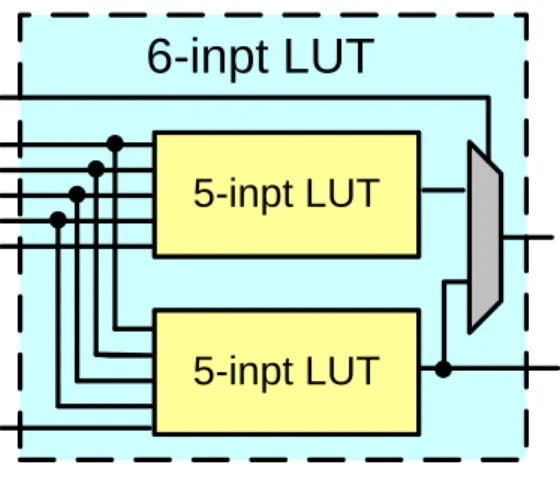
Practically, basic logic cells on modern FPGAs are flexible. In other words,

modern FPGAs employ two single-output LUTs with shared inputs as shown in

Figure 3.5. In general, this kind of circuits is called two-output LUTs. We observe that

two-output LUTs can map two single-output Boolean functions simultaneously if the

two functions satisfy two conditions: (i) the summation of the two function’s distinct

variables should be fewer than or equal to the physical-input constraint denoted as

PIC (PIC8 on Altera Stratix IV, and PIC5 in Xilinx Vertex V, e.g., PIC is equal to 6 in the example as shown in Figure 3.5), and (ii) the summation of the LUT

size of the two functions should be fewer than or equal to the The covered penultimate

stratum dot plane

Delete the redundant match m

Phase I complete

Any redundant match m in the penultimate stratum dot plane dz-1

Yes No

physical-capacity constraint denoted as PCC (PCC64 on Altera Stratix IV, and 64

PCC in Xilinx Vertex V [1, 2]) . Actually, PCC is equal to 2K, where K is the input constraint of a LUT. Besides, a two-output LUT can map a single output

function if the number of variables of the function is K (K = 6) as shown in Figure 3.5.

Moreover, we can merge the two distinct LUTs among all strata if the two functions

mapped by these two distinct cells satisfy PIC and PCC. Suppose we want to map the

two prime patterns p4 1, 2p as shown in Figure 3.6(a) (i.e., PIC6 , 64

PCC ), and then we can map the two patterns onto four two-output LUTs as shown in Figure 3.6(a). Obviously, the summation of the number of inputs of LUT 2

and 4 is equal to 6 which is fewer than PIC, and the summation of the LUT size is

equal to 3 3

2 2 which is fewer than PCC. Hence, we can merge LUT 2 and LUT 4 into a single LUT as shown in Figure 3.6(b). In Phase II, we merge the distinct LUTs

to map different patterns if these two functions mapped by them satisfy PIC and PCC.

5-inpt LUT

5-inpt LUT

5-inpt LUT

6-inpt LUT

LUT1

LUT 3

LUT 2

LUT 4

p

p

p

p

LUT 2

_{LUT 1}

LUT 3

(a)

(b)

Chapter 4

Experimental Results

4.1 Experimental Information

We implement DOCT and the GPC heuristic [14] in C/C++ language on a

workstation with an Intel Xeon 2-GHz processor and 16 GB main memory under

the Centos 5.2 operating system. Besides, an open source package, lp_solve 5.5.13,

is used to solve the linear formulations. A set of benchmark circuits is evaluated

including three Radix-4 unsigned Booth-encoded multipliers (8 by 8 and 16 by16),

multiplier accumulators (MAC), discrete cosine transformation (DCT) [20], finite

impulse response filters (FIR), and motion estimations (ME). The input of each

compressor trees is extracted from the simulation result produced by MATLAB

Simulink toolbox. All compressor trees in our experiments are directly synthesized

without pipelined.

Table I illustrates the detail information of the benchmark circuits. In Table I,

Column 1 shows the variety of our benchmark circuits. Column 2 and Column 3

show the width and the height of the input dot plane, respectively. Column 4 shows

4.2 Parameters Setup

We implement two compressor tree synthesis algorithms DOCT and the GPC

heuristic. The following is the setting of parameters in our experiment.

DOCT: Compressor tree synthesis using DOCT described in preceding sections

under K6 and H3. This thesis supposes that DOCT is evaluated on Altera Stratix IV. Thus, the physical input constraint (PIC) is set to 8 and the physical

capacity constraint (PCC) is set to 64. The compressor tree produces three outputs

summed by ternary adder.

GPC: Compressor tree synthesis using the generalized parallel counter (GPC)

heuristic. In the GPC heuristic, there are three parameters: (i) M is the input

TABLEI CIRCUIT INFORMATION

Circuit Width Height Total

8 by 8 16 5 56 16 by 16 32 9 176 DCT_1 22 10 150 DCT_2 20 6 83 DCT_3 20 5 82 DCT_4 20 8 116 DCT_5 22 7 105 FIR_1 15 9 72 FIR_2 23 13 167 FIR_3 39 21 374 ME_1 10 10 100 ME_2 14 14 196 MAC_1 9 6 34 MAC_2 11 7 47

constraint of GPC patterns (the input constraint of LUTs in the targeted FPGA, e.g.,

6 for Altera Stratix IV, and Xilinx Vertex V), (ii) N is the output constraint of GPC

patterns, and (iii) k is the number of inputs of the final CPA (i.e., k is equal to H). In

our experiments, M is set as 6; N is set as 4; k is set as 3. The setting is the same as

[14].

4.3 Experimental Results

In our experiment, we compare both the depth and area produced by DOCT to

that by the GPC heuristic. Table II, III, and IV show the experimental results under

TABLE II

SYNTHESIS RESULT UNDER K = 5 K = 5 Circuit UB delay LUTs DOCT GPC DOCT GPC 8 by 8 1 1 2 29 45 16 by 16 3 2 4 149 222 DCT_1 3 3 3 160 171 DCT_2 2 2 2 103 109 DCT_3 1 1 1 42 47 DCT_4 2 2 2 101 107 DCT_5 2 2 3 86 132 FIR_1 3 2 4 61 97 FIR_2 3 3 4 177 222 FIR_3 4 4 4 536 580 ME_1 3 3 3 107 110 ME_2 4 3 4 222 240 MAC_1 2 1 3 17 40 MAC_2 2 2 3 34 50 Avg. 0.83 0.73 1 0.83 1

different input constraints of LUTs: K 5, K6, and K7, respectively. In Table II, III, and IV, Column 2 illustrates upper bounds of all benchmark circuits.

Column 3 and Column 4 illustrate the depth of compressor trees produced by

DOCT and the GPC heuristic. Meanwhile, Column 5 and Column 6 illustrate the

area in terms of LUTs on Altera Vertex Stratix IV produced by DOCT and the GPC

heuristic. Compared to the GPC heuristic, DOCT has 27% less depth with 17%

fewer LUTs under K5; 32% less depth with 21% fewer LUTs under K6; and 20% less depth with 2% fewer LUTs under K7. For all benchmark circuits, the GPC heuristic was finished in few seconds; meanwhile, DOCT was finished in

500 seconds.

TABLE III

SYNTHESIS RESULT UNDER K = 6 K = 6 Circuit UB delay LUTs DOCT GPC DOCT GPC 8 by 8 1 1 1 24 30 16 by 16 2 2 3 132 174 DCT_1 2 2 3 127 152 DCT_2 2 2 3 98 120 DCT_3 1 1 2 35 70 DCT_4 2 2 3 90 118 DCT_5 2 2 3 66 104 FIR_1 2 2 2 52 58 FIR_2 3 2 3 131 160 FIR_3 3 3 4 400 459 ME_1 2 2 3 78 105 ME_2 3 3 4 174 193 MAC_1 1 1 2 16 26 MAC_2 2 1 2 19 38 Avg. 0.73 0.68 1 0.79 1

It is evident that DOCT always have better or the same result in depth

compared to the GPC heuristic. The reason is that DOCT consider all combinations

of all prime patterns for constructing a compressor tree. Although DOCT does not

outperform the GPC heuristic in area for every case, it provides smaller area on

average.

TABLE IV

SYNTHESIS RESULT UNDER K = 7 K = 7 Circuit UB delay LUTs DOCT GPC DOCT GPC 8 by 8 1 1 2 26 40 16 by 16 2 2 2 125 119 DCT_1 2 2 3 109 127 DCT_2 2 2 2 83 78 DCT_3 1 1 2 40 62 DCT_4 2 2 2 82 78 DCT_5 1 1 1 44 44 FIR_1 2 2 2 51 48 FIR_2 2 2 3 125 135 FIR_3 3 3 3 397 334 ME_1 2 2 2 78 69 ME_2 2 2 3 123 153 MAC_1 1 1 1 12 16 MAC_2 1 1 2 22 33 Avg. 0.8 0.8 1 0.98 1

Chapter 5

Conclusions and Future Work

A delay optimal compressor tree synthesis algorithm, DOCT, has been

presented in this thesis. Since the infinite set of patterns can be superseded by the

finite set of prime patterns without loss of delay optimality, DOCT adopts an

ILP-based methodology to map prime patterns onto the compress tree with the

minimum depth and utilizes a post-processing procedure to minimize area overhead.

Therefore, DOCT can authenticallyarchive compressor trees with minimum depths

by all prime patterns under the input constraint of a LUT. On average, compressor

trees produced by DOCT have 32% less depth and 21% fewer LUTs than those

produced by the GPC heuristic on modern technologies.

Although DOCT has made a progress in reducing area overhead compared

to the GPC heuristic, we believe that there is still room for improvement. In the

beginning, we have put the area cost in the cost function of ILP formulation.

Unfortunately, the run time of DOCT is too long and unacceptable. But according

to the result of some smaller case, DOCT considering area cost in the cost function

could archive around 50% fewer LUTs than that does not consider. Yet, we believe

Reference

[1] Altera Corporation, Stratix IV device handbook. [Online]. Available: http://www.altera.com/

[2] Xilinx Corporation, Vertex-5 FPGA user guide. [Online]. Available: http://www.xilinx.com/

[3] Altera Corporation, Stratix III device handbook. [Online]. Available: http://www.altera.com/

.

[4] Xilinx Corporation, Vertex-4 FPGA user guide. [Online]. Available: http://www.xilinx.com/

[5] M. C. Herbordt, T. VanCourt, Y. Gu, B. Sukhwani, A. Conti, J. Model, and D. DiSabello, “Achieving high performance with FPGA-based computing,”

Computer, vol. 40, no. 3, pp. 50–57, March 2007.

[6] Altera Corporation, FPGAs provide reconfigurable DSP solutions. [Online]. Available: http://www.altera.com/literature/wp/wp_dsp_fpga.pdf

[7] S. Mirzaei, A. Hosangadi, and R. Kastner, “FPGA implementation of high speed FIR filters using add and shift method,” International Conference on Computer

Design, October 2006, pp. 308–313.

[8] O. Kwon, K. Nowka, and Jr. Swartzlander, “A 16-bit by 16-bit MAC design using fast 5:3 compressor cells,” Journal of VLSI Signal Processing Systems, Vol. 31, No. 2, pp. 77-89, June 2002.

[9] C.-Y. Chen, S.-Y. Chien, Y.-W. Huang, T.-C. Chen, T.-C. Wang, and L.-G. Chen, “Analysis and architecture design of variable block-size motion estimation for H.264/AVC,” IEEE Transaction on Circuits and Systems, vol. 53, no 2, pp. 578-583, February 2006.

[11] C. S. Wallace, “A suggestion for a fast multiplier,” IEEE Transaction on

Electronic computers, vol. 13, no. 1, pp. 14–17, February 1964.

[12] V. G. Oklobdzija, D. Villeger, and S. S. Liu, “A method for speed optimized partial product reduction and generation of fast parallel multipliers using an algorithmic approach,” IEEE Transaction on Computers, vol. 45, no. 3, pp. 294–306, March 1996.

[13] P. F. Stelling, C. U. Martel, V. G. Oklobdzija, and R. Ravi, “Optimal circuits for parallel multipliers,” IEEE Transaction on Computers, vol. 47, no. 3, pp. 273–285, March 1998.

[14] H. Parandeh-Afshar, P. Brisk, and P. Ienne, “Efficient synthesis of compressor trees on FPGAs,” Asia South Pacific Design Automation Conference, March 2008, pp. 138–143.

[15] H. Parandeh-Afshar, P. Brisk, and P. Ienne, “Improving synthesis of compressor trees on FPGAs via integer linear programming,” Design Automation and Test

in Europe, March 2008, pp. 1256–1261.

[16] P. S. Zuchowski, C. B. Reynolds, R. J. Grupp, S. G. Davis, B. Cremen, and B. Troxel, "A hybrid ASIC and FPGA architecture," International Conference of

Computer-Aided Design, November 2002 , pp. 187-194.

[17] A. Cevrero, P. Athanasopoulos, H. Parandeh-Afshar, A. K. Verma, P. Brisk, F. K. Gurkaynak, Y. Leblebici, and P. Ienne, “Architectural improvements for field programmable counter arrays: enabling efficient synthesis of fast compressor trees on FPGAs,” International Symposium on Field Programmable Gate

Arrays, February 2008, pp. 181–190.

[18] P. Brisk, A. K. Verma, P. Ienne, and H. Parandeh-Afshar, “Enhancing FPGA performance for arithmetic circuits,” Design Automation Conference, June 2007, pp. 334–337.

[19] J. Cong and Y. Ding, “FlowMap: an optimal technology mapping algorithm for delay optimization in Lookup-Table based FPGA designs,” IEEE Transaction

on Computer-Aided Design of Integrated Circuits and Systems, vol. 13, no. 1,

[20] W. Pan, A. Shams, and M. A. Bayoumi, “NEDA: a new distributed arithmetic architecture and its application to one dimensional discrete cosine transform,”

IEEE Signal Processing Systems, October 1999, pp. 159–168.