A hierarchical system for dynamically solving planning and scheduling problem in a flexible manufacturing system

(1)

A

Hierarchical System for Dynamically Solving Planning

and Scheduling Problem in a Flexible

Manufacturing S

ys tem

Pei-Sen

Liu arid Li-Chen

Fu

Department of Computer Science

&

Information Engineering

National Taiwan University, Taipei, Taiwan, R.O.C.

ABS

T R

ACT

There are inevitably time-varying factors exkting in a flexible manufacturing system ( FMS ). In this paper, a system with a two- level structure ( high and low level ) for dynamically solving the problem of planning and scheduling in an FMS altogether is presented. The problem is first formulated as the determination of an optimd routing assignment of p automated guided vehicles ( AGV's ) among m workstations to accomplish N tasks, facing several possible dynamical situations, e.g. change of due date or breakdown of some workstation(s). The hierarchical system is then built to solve this optimization problem in a dynamical manner. The low level aims to solve the routing problem for AGV's among

workstaions given a set of AND/OR graphs which represent tasks

to be processed. On the other hand, the high level, via a rule based system, provides necessary data for low level use and simultane- ously determines principles as how to respond to occurrence of some unexpected events. It is shown that a near-optimal solution can be derived with moderate computation time, which allows operation in an FMS to be more flexible.

I. Introduction

An FMS is a large complex system consisting of many inter- connected components of hardware and software [ 1][2]. The necessary planning and decision control of an FMS include balancing the workload, responding to changes, scheduling and dispatching, and managing tools and materials, etc. Several aspects of current FMS planning and decision control system have been discussed in [2]-

[61.

In an FMS, a workstation ( o r so called cell) is d e h e d as the smallest building block of the system consisting of a computer con- trolled machine. A basic design principle of an FMS is to have as

many identical workstations as possible to enhance flexibility. Therefore, there may be more than one sequence of operations to produce a part, which implies that "planning" on the choice of a sin- gle sequence out of all possible candidate sequences has to be performed. In addition, it is the AGV that are responsible of carrying

workpieces among workstations for each operation. Hence a good scheduling method will be required to determine the routing assignment for AGV's. But as has been known that the complexity of

solving this problem is considerably high if its so called "optimal" solution is attempted. Thus, introduction of some good heuristics so

as to reduce the complexity would be more favorable, especially in a dynamic environment such as an FMS where occurrence of unexpected events is usual.

Several approaches to planning. decision control, and scheduling of an FMS have been suggested in [7]-[12],[16]. However, the proposed works either can not solve the problem of planning and scheduling dynamically, or are not suitable for solving the routing problem of AGV's in an FMS.

This paper formulates the problem of dynamic planning and scheduling as the one of determining the optimal routing assign- ment of p AGV's among m workstations to accomplish N tasks in

an FMS. The approach used here is a hierarchical and dynamic one which solves the problems of planning and scheduling as a whole. Especially it can handle some occasional situations such as break- down of some workstation(s), as well as can respond to some changes, for example, of production target.

The paper is organized as follows: in section 11, we formulate the problem and describe the optimality criterion for the solution; in section 111, we briefly introduce the structure of our hierarchical planning and scheduling system, and describe the necessary information for the system; in section IV, we explain how the low level

subsystem works and the techniques used in this level, including A' search algorithm and minimax strategy; in section V. we describe the function of the high level subsystem and its most h p o r t a n t rule based system; in section VI, some computational results are shown to illustrate the performance of this hierarchical system.

11. Problem Formulation and Optimality Criterion

The main problem in an FMS is usually divided into two parts: planning, or process routing, which is the selection of a sequence of operations; and scheduling, which is the assignment of time and resources. Here we define our problem as the determina- tion of an optimal routing assignment of p AGV's among m works-

tations to accomplish N tasks in order to minimize the total completion time.

Suppose there are k kinds of the total N tasks and the number of the ith kind is Ni, 15 i s k, so that N = N,+N,+

...+

N,. Each task is to let an AGV carry necessary materials (parts or subparts)

and to follow the assigned route among workstations so that every subtask of the task can be successfully processed by the selected workstations. Thus, to complete N tasks the routes for total p

AGV's among m workstations have to be assigned. Moreover, the

total completion time of a task is the sum of total execution time (through workstations), total travelling time of an AGV (among

workstations), and total waiting time (when two or more AGV's arrive at the same workstation). Now due to the fact that each task will require a sequence of processing by some selected workstations, performing the routing assignment is equivalent to solving the

77

(2)

problem of planning. Later in the sequel, how to minimize the total completion time will be shown to be our main consideration for assigning routes for those AGV's. This indicates that, from our pre- vious definition, the planning problem can also be treated as a scheduling problem. Consequently, we can define the problem of planning and scheduling together in an

FMS

as the routing assignment problem. The following are necessary assumptions.

Assumptions :

materials necessary for all kinds of tasks.

I) All AGV's are the same. Every AGV can carry all kinds of

2) All AGV's are travelling at constant known speed. 3) The travelling time for each AGV between workstation Wi, W,. and W, satisfies the triangle inequality.

4) All workstations along with all paths connecting them form a complete graph[l8]. Each path can accommodate only one A G V at a time.

5 ) There are no precedence constraints between any two tasks, but every task can be decomposed into some related subtasks. The general AND/OR graph [13][14] is used to represent these subtasks [18].

6) The number of every part to be produced and the due date for every kind of part are given at any time, but may subject to variation as the manufacturing proceeds.

7) Tasks are nonpreemptive.

The design of a mathematical model for the routing assignment problem follows the steps shown below.

A. Representation of t h e System Model

A material haadling system of aa

F M S

can be represented by a triplet S = ( A , W , T ), in which the arguments represent the set of AGV's , the set of workstations, and the set of tosk graphs respectively. Specifically, A = ( v l , v 2 ,

....

vp

1,

where vi denotes the ith AGV, and all p AGV's are the same except that they may run at different speed; W = (

W

,,

....

W,,

W q + l .

....

W,

1,

where W ; , I < i l q. denote the real workstations and W,, q + l < j S m,

denote the terminals for AGV's (loading and unloading places); and T = ( T I . T2,

....

T t , N I , N2.

....

N k , D 1 , D 2 .

....

Dt

1,

where T , , N;, and Di denote respectively the AND/OR task graph, the number of task, and the due date of the i t h kind of task, IS il k,

Remarks: ( I )

a n d N = N I +

...+

Nk.

Later in the sequel, we will not distinguish the real worksta- tions from terminals, and simply call W, the i t h workstation, 1S i l m.

We further denote Ti = ( V i , E; ), rhe ith task graph, where V i represent the set of vertices and E; the set of directed links.

Let

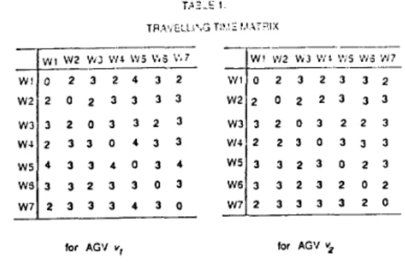
WTT'

be the symmetric matrix to represent the travelling time between any two workstations for AGV v,, where the entry W T T ' ; , , denotes the travelling time spent by that AGV when it travels from workstation i to workstation j, I5 i , j l m. Every task graph T , = ( V i , Ei ) is an general AND/OR graph with directed edges. The directed edge from vertex i to vertex j indicates that the subtask to be processed by workstation i must go before the subtask to be processed by workstation j. An OR branches indicates that only one of the subtasks which immediately follow the branch

(2)

needs to be done. An AND branches indicates that all subtasks following the branch should be completed but the order is not impor- tant (since there are no precedence or dependency relationship among them).

B. Cost Function

The cost function for a particular task when assigned to certain AGV is the sum of the aforementioned execution time, travelling time, and waiting time spent by that AGV. Now suppose that the AGV v i is assigned to perform tasks til,

....

tlpi sequentially, then its travelling sequence. is denoted 0' = ( Oil, 0 l 2 .

....

0'") where

01

E W, 1 S j l ni, and ni is the total number of workstations travelled. Given this notation, we are now ready to define travelling time, execution time, and waiting time throughout a task execution by an AGV, say, vi in detail as follows.

Definition 1: Let TT', denote the time spent by the AGV vi when travelling from workstation 0'; to workstation O\+l out of the sequence 0'. 15 j S (q-1). Then the travelling time of v; to accomplish the sequence of tasks til.

....

tipi is defmed as:

" . - I

TT' = TT;

) = I

Definition 2: Let Eii denote the time required by workstation 0; to complete its processing, 1 5 j S ni Then the task execution time corresponding to the travelling sequence 0' is deEned as:

D.

) = I

Definition 3: If AGV vi and AGV vi arrive at a workstation at the same time or a workstation is doing some subtask for AGV vi when AGV vi arrives, then either of the two AGV's, vi and v,. has to wait or vi has to wait till the workstation finishes the current sub- task. Hence we let WTIk be the waiting time of the AGV v; at the workstation Oik from the travelling sequence 0' so that the total waiting time of the AGV vi to complete the travelling sequence 0' is defined as: W T ' = z W T \

n

i = l

A s a result of the above definitions, the total completion time TAS) spent by the AGV vi corresponding to the routing assign- ments S for all AGV's is the sum of travelling time, task execution time, and waiting time as follows:

Ti( S ) = TT'

+

ET'

+

WT' Sys!em Input Informa!ion

.. ...

711m

(Same Algorithmic Techniques)

I

...

z

A New Raul:nQ Assignment

Planning and Scheduling System. Figure 1. The Structure of the Dynamic Hiererchical

(3)

TPZ-C 1

~p.”,~:Ll~.GTI!.:~!,~~;”iX

_

~

-

~

for AG’I v, for AG‘I 5

C. Optimnlity Criterion

Let Q denote all possible routing assignments for p AGV’s to accomplish all tasks before due dates. Then our optimality criterion is to find an optimal routing assignment S such that:

S = a r p i n ( max(T,(S’))

I

sen 1 5 % ~

It is well known that this problem is an NP-complete problem. Moreover, the environment of a manufacturing system may be changing dynamically. Therefore, it may be impractical to spend a lot of time to find an optimal assignment in advance of real running. Therefore, we will use a dynamic method to find a “near optimal” solution.

111. A Hierarchical Planning and Scheduling System

To dynamically solve our problem, in this section, we propose a hierarchical system whose structure and environment is shown in Figure 1. More detaded explanations are given in the following. A. System Input :

tem can be classified into the following two groups: ( 1 ) Inirial Information :

The information that should be input to the hierarchical sys-

This describes the initial state of the environment of an FMS, but it may be changed afterwards. It usually includes the fol-

task 1 task 2 task 3

yw5

Figure 2. AND/OR Task Grephs.

t a s k 1 t a s k 2 task 3

D%L: 5 7 0 0 5 3 5 0 4000

Table 2 . Task I n f o r m a t i o n .

lowing:

(1) position of each workstation; (ii)

(iii) number of total AGV’s; (iv) travelling speed of each AGV;

( v ) current number of products of each kind to be manufactured;

(vi) manufacturing process and due date of each kind of product;

For illustration, we give an example of such input information in Table 1.2 and Figure 2, where the former indicates the necessary information about workstations and AGV’s through travelling time matrices whereas the latter describes those about each kind of products. In this example, the FMS includes two AGV’s, seven workstations, and three different kinds of tasks. In particular, the numer- ics in each node of graphs in Figure 2 denotes the amount of execution time needed in the corresponding workstation.

( 2 ) Occasional Events :

distance between any two workstations;

These events may occur occasionally but unexpectedly due to the dynamic nature of an FMS. They include the following:

(1)

(ii) breakdown of some workstation(s); (iii) change of position of some workstation(s); (iv) change of due date(s) of some product(s);

( v ) addition of another kind of product to be manufactured; change of the condition of some AGV( ‘s);

B. System Structure

The hierarchical system is a two-level structure, namely, a high level subsystem on the top of the low level one. Their respective functions and solution techniques are described as fol- lows.

( 1 ) High Level :

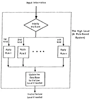
This level can be regarded as the decision supporting part of the overall system. Two kinds of problems to be solved here are the following: ( I ) Given an A G V which is freed at a particular instant of time ( either because it has just carried out a task or because it is newly added in ), which unprocessed task should be assigned to it ? ( 2 ) When some occasional event(s) suddenly occur, what kind of correction to the already determined routing assignment should be enforced ? Since this level involves the problems with policies and with unpredictable events, it is seen to be more efficient to use some heuristic techniques to solve them. Therefore, a rule based system using forward chaining control is adopted here as the main solution technique of this subsystem.

( 2 ) Low Level :

The problem for this level can be precisely phrased as follows: When each A G V is assigned to one of the tasks ( several could be of the same kind ) to be processed ( due to the decision made in the high level ) and given the most current state information of the environment, what are the optimal routes for a l l the AGV’s SO that the previously mentioned optimdity criterion is to be or close to be achieved. Clearly, this problem is fairly a deterministic one and, hence, algorithmic techniques are preferable for solving it. This, then, leads to our choice of A‘ search algorithm and minimax stra- tegy as the solution technique in this level.

(4)

Input lnforiralion IV. Low Level Algorithmic Method

The structure of this level is shown in the diagram in Figure 3. AU the data are stored in the data base which includes the follow-

ing: 1) the current position and the condition (free or busy) of each available AGV, 2) the state of every workstation, 3) the kind of task to which each AGV is assigned, and 4) the AND/OR graph of

eveiy task. These data are frequently updated through the high level instructions to reflect the current environment. With the most current information stored, the low level then solves the routing problem via an algorithmic method.

Before the routing assignment problem can be solved, it is more convenient to transform it into a state space search problem so that the powerful A’ algorithm[14] and minimax strategy[lS] can

be used. In this level, the problem to be treated here is only a part of the whole original problem. The solution in this case is simply an optimal routing assignment for p AGV’s among m workstations to

accomplish p tasks ( in contrast with the original N tasks ). The state space search method for this level and the heuristic estimation procedure are stated in [17][181.

After computing the heuristic cost of every node in the task graph for all AGV’s, we can then calculate every cost estimate fi(n)

for every AGV vi at run time. Finally, since the evaluation function f(n) defmed before satisfies the minimax strategy, i.e.:

f(n) = maxfi(n)

K S p

our principle for expanding nodes in A’ search algorithm will obtain

an optimal solution. Now we have shown how to solve the fixed problem by using A’ search algorithm and minimax strategy in the

low level of our system.

By assumption 4). every passage connecting one workstation to another can allow AGV’s running only in one direction at a time.

If an AGV is already on that passage and is heading toward a workstation while the other AGV is ready to leave that workstation

by that passage but with converse direction, the the waiting time for the departing AGV should be accounted for in the calculation of

the evaluation function. But when more than two AGV are running

on the same passage and the one in the rear is running at a faster speed than that of the one in the front, similar waiting time should also be considered.

The Hiph Level

Collect Ihe necessary data and call the low level

,...

.

...

!

I

i

L

.

i -...............-........,...

...

:

1

A New Routing Assignment F i g u r e 3. T h e Structure of t h e Low Level.

‘.

. ...

.-..

....

Dala Ease for tha Low Leiel if needed

lnvcie the Law

Level if needed

...

....

...

Figure 4. The Structure of the tiiph Level.

V. High Level Heuristic Method

This level is responsible for making decisions and sending useful data to the low level subsystem. Figure 4 shows the structure of this level whose process flow can be summarized into the following steps: Step 1. Step 2. Step 3. Step 4. Step 5 .

Identify the occasional event(s) which just occur(s): Change the information about the entire environment; Take some proper measures to handle the event; Update the data base of the low level subsystem; Invoke the low level if necessary to obtain a new routing assignment.

A. Basic Method

Whenever some occasional event occurs, including that where some task has been just completed, the optimality principle will require that

all

the subtasks which are in process or ready to be processed be taken into reconsideration. This means that if some

AGV, say, vi is assigned a task with its corresponding AND/OR

graph containing rn, nodes, V I ,

.... V,,,,, and currently this AGV is

performing the subtask corresponding to the node Vi ( I < i,< m,), then we must consider all the Following subtasks corresponding to nodes Viw,

...

V,,,, together in order to find a better routing assign-

ment. Hence, the predetermined route for AGV vi may be changed after a new invoke of the routing assingment process of the low level. A detailed procedure used to update the data base, especially

the state description, of the low level subsystem is given in [18].

B. Rule Based System

One of the major functions of the high level subsystem is to handle occasional events and make responses. Since these events vary drastically, their handling processes are considerably different. Therefore, it is especially appropriate to use a rule based system (

(5)

( P rule1

( ac:.noiv!edpe the chanfie of dJe da:e of some k h d of proddct) ( upda!e the due dale)

( notlfy tcle supervisor) ”>

) ( P rule2

( a n AGV is freed from i!s procedinp task) ( upda:e the coidllion 01 that AGV)

( reduce the number of !he unprocessed tasks 01 the s a n e kind)

( assign this AGV t o Some unprocessed task by same heuris!;cs) ( upda!e the data base 01 the b w lwei subsyslem)

( iivcke the roJlinp assignment process 01 the IOW level) - - >

1

( P rule3

( a worisla!ion breaks dDwn)

( change the ini!ial information about the sys!em)

( nc!i‘y tCe supervisor) ( sand Harning sigqal)

( updale !he da!a base of the low level sdbsys!em)

( invcie the r o u h p assipnment process of the low level) -->

)

Fig,.re 5. Exernp!es of Production Rules

consisting of production rules ) as shown in Figure 4 to deal with this situation. The production rule is, in general, of the following form :

I F < c 0 n d . b ... < cond.n> THEN < act.l>

...

< act.m> For illustration, examples of the production rules are given in Figure 5 . Among them, the first one express the subsequent action when the due date of some kind of product is changed; the second one lists a set of measures whenever an AGV is freed from its preceding task; the last one takes care of the situation where the breakdown message of any workstation is received. In the first example, no immediate invoke of a new routing assignment process is needed, but the rest of two examples will require such a reaction to get a new routing assignment

For a number of other similar situations, analogous production rules can be generated. Hence, it is this rule based system which makes the overall planning and scheduling system extremely dynamic.

VI. C o m p u t e r S i m u l a t i o n E x a m p l e s

In this section, we implement a simulation program of the hierarchical planning and scheduling system on VAX 8530. Com- parison between results of our approach and those from the other methods is performed and shown. For simplicity, we assume there is no occasional event which occurs unexpectedly so that the FMS is running in a normal situation. The necessary information about the problem is given in Table 1 , 2 and Figure 2, and the simulation results are shown in Table 3. In the first column of Table 3, there are four different kinds of methods and each with six different conditions ( about different due dates and different heuristics ) listed in the first row. The details about these methods and conditions are: Methods:

( I ) Use the hierarchical planning and scheduling system presented in this paper to solve the problem as shown in Figure 2. ( 2 ) Use a method similar to ( I ) with the difference described as

follows: whenever an AGV is freed, a new task is assigned to it and a new route for that AGV is established through the use of

t a s k 1 t a s k 2 t a s k 3

Q

p

1 1 W I t a s k 1 t a s k 2 t a s k 3 * 7 U7

j 2

( b ) F i x e d S e q u e n c e 2 T:?l?ra 6 . T K O T i x e a T r a v e l ! i n g S e q l l e n z e r .

A’ search algorithm, but all predetermined routes for other busy AGV’s remain unchanged.

( 3 ) The method here is similar to ( I ) except that processing sequence to accomplish every kind of task is k e d as shown in Figure 6(a).

( 4 ) This method is similar to (3) but the processing sequence is now changed as shown in Figure 6(b).

Conditions:

( I ) Different due dates : Three different types of due dates for three kinds of tasks are assumed.

A rule bused ?stem : The rules contained here involve the due dates, the estimated completion time, and the number of every kind of tasks.

Earliest Due Date ( E D D ) Principle : The processing order of different kinds of tasks is based on the knowledge of due dates.

The measures used here are the total time spent to accomplish every kind of task and that to accomplish all these tasks. The test results show that our system with AND/OR task graphs (method 1) performs much better than the others. In addition, our rule based module is preferable to the EDD principle, since some results given by EDD principle can not even finish all the tasks before the due date as opposed to ours. Moreover, since the number of AGV’s in a real FMS is usually small, and the computer run-time spent in A‘ search algorithm heavily depends on the number of total AGV’s and the size of every task graph, the total computational time can.

(6)

Thcducdueia Thcducdueb

780.680.510 600.780.600

w = I Y -dYdY

&- EDDnJc Rulc-Brpad EDDnJe

712 8.25 560 617 m 6 4 9 7 C d s o s w 455 8 9 455 810 807 7M 629 746 647 834 827 595 448 163 448 955 961 7Cd 161 811 773 941 971 572 589 725 591 839 841 643 641 674 663 842 842 511 465 613 * ~5 I I

in fact, be more satisfactory. Consequently, this method constitutes a promising planning and scheduling algorithm in a real environment of an FMS.

VII.

Conclusion

In this paper, the problem of planning and scheduling altogether in an FMS is formulated, as the determination of an optimal routing assignment for automated guided vehicles. Due to the dynamic nature of an FMS, a hierarchical system is built to solve this routing assignment problem in a dynamic manner. Such a system integrates the advantages of both algorithmic and heuristic techniques and, hence, can be more general and more efficient. For illustration, computer simulation examples are provided and their results shown in Table 3 are, in fact, quite satisfactory. Further- more, since the number of AGV's in an FMS is usually very small, the total computational time is also economical. Therefore, applica- tion of this method to an FMS in a real environment will be quite promising.

References

Simpson, J. A., R. J. Hocken, and J. S. Albus, 'The automated manufacturing research facility of the National Bereau of Standards," J. Manuf. Syst.. vol. I , pp. 17-32, 1982. Sui, R. and C. K. Whitney, "Decision supporting requirements

in flexible manu-facturing," J. manuf. Syst., vol. 3 , no. 1, pp. 61-69, 1984.

Chen, P. E. and J. Talavage, "Production decision support system for computerized manufacturing system," J. Manuf. Syst.,

Whitney, C. K., "Integration in FMS design and control," in Proc. ASME Computer in Engineering Conf.. pp. 355-360, 1986. Young, R. E., "Planning and control requirements for flexible manufacturing systems," in Proc. ASME Computers in Engineering Conf., pp. 347-353, 1986.

Ballakur, A. and H. J. Steudel, "Integration of job shop control systems: A state-of-art review," J. Manuf. Syst., vol. 3, no. Stecke, K. E. and T. L. M O M , 'The optimality of balancing workload in certain types of flexible manufacturing system," Europe. J. Oper. Res., vol. 20, pp. 66-72, 1985.

Ho, Y. C. and

X.

R. Cao, "Performance sensitivity to routing changes in queuing networks and flexible manufacturing systems using perturbation analysis," IEEE J. Robotics Automa- tion. vol. RA-I, no. 4, Dec., 1985.

Bermen. 0. and 0. Maimon, "Cooperation among flexible manufacturing systems," IEEE J. Robotics and Automation. vol. RA-2, no. 2, pp. 24-30, Mar., 1986.

Fox,

B.

R. and K. G. Kempf, "Opportunistic scheduling for robotics assembly," in Proc. IEEE Inter. Conf. on Robotics and Automation. pp. 880-889. 1985.

Xiaodong Xia George A. Bekey. "SROMA: An adaptive scheduler for robotic assembly system," in Proc. IEEE Inter. Conf. on Robotics and Automation, pp. 1282-1287, 1988. Jane C. A., T. Govindaraj, and M. M. Christine, "Decision models for aiding FMS scheduling and control," IEEE Truns. Syst. Man Cybern., vol. 18, no. 5 , pp. 744-756, SepJOtc., 1988.

L. S. Homem de Mcllo and A. C. Sanderson, "AND/OR graph representation of assembly plans," in Proc. AAAI. pp. 1113-1119, 1986.

N. J. Nilsson, Principle of Arhifrcial Intelligence, Palo Alto, CA: Tioga, 1980.

Shen, C. C. and W. H. Tasi, "A graph matching approach to optimal task assignment in distributed computing systems using a minimax criterion," IEEE Trans. Comput., vol. C-34,

Chun, C. L., C. S. George and C. D. Mcgdlem,

'Task

assignment and load balancing of autonomous vehicles in a flexible manufacturing system," IEEE J. Robotics and Automation vol. RA-3, no. 6, Dec., 1987.

Liu, Pei-Sen and L. C. Fu, "Planning and scheduling in a flexible manufacturing system using a dynamic routing assignment method for automated guided vehicles," in Proc. IEEE Inter. Conf. on Robotics and Automation, May, 1989.

Liu, Pei-Sen and L. C. Fu, "A Hierarchical System for Dynamically Solving Planning and Scheduling. Problem in Flexible Manufacturing System." Technical Report NUTCSIE 88-05. Department of Computer Science and Information Engineering, National Taiwan University, 1988.

vol. I, no. 2, pp. 157-168, 1982.

1, pp. 71-88, 1984.