粒子濾波算法應用在多輸入多輸出天線正交分頻多工的訊號檢測之研究

國 立 交 通 大 學

電信工程學系

碩 士 論 文

粒子濾波算法應用在多輸入多輸出天線正交分

頻多工的訊號檢測之研究

A Study on Data Detection using Particle Filtering

in MIMO-OFDM System

研究生：陸裕威

指導教授：黃家齊 教授

粒子濾波算法應用在多輸入多輸出天線正交分

頻多工的訊號檢測之研究

A Study on Data Detection using Particle Filtering

in MIMO-OFDM System

研 究 生：陸裕威 Student： U-Wai Lok

指導教授：黃家齊 Advisor：Dr. Chia-Chi Huang

國 立 交 通 大 學

電信工程學系碩士班

碩 士 論 文

A Thesis

Submitted to Department of Communication Engineering College of Electrical Engineering and Computer Engineering

National Chiao Tung University in partial Fulfillment of the Requirements

for the Degree of Master

in

Communication Engineering August 2008

Hsinchu, Taiwan, Republic of China

粒子濾波算法應用在多輸入多輸出天線正交分

頻多工的訊號檢測之研究

學生：陸裕威 指導教授：黃家齊

國立交通大學電信工程學系 碩士班

摘

要

在多輸入輸出正交分頻多工的系統上，由於訊號之間的干擾，因此在接

收端要做訊號的檢測的複雜度比單接收天線時的正交分頻多工系統來得複

雜。特別是利用最大概似法(ML)作訊號檢測時，接收機的複雜度將會隨着

天線的數量的增加或調變的不同呈現指數的增加。這篇論文主要是利用粒

子濾波算法應用在多輸入多輸出正交分頻多工的訊號。粒子濾波算法利用

統計的原理，造出相對應的事後機率用以作訊號檢測，來達到接近最大概

似法的效能的同時減低複雜度。我們再使用一些方法合併粒子濾波算法去

得到接近最大概似法的效果，在模擬顯示出粒子濾波演算法的結效能和我

們提出的一些改良方法的效能比一般的 VBLAST MMSE OSIC 更接近最大概似

法的效能，而且其複雜度遠少於最大概似法。

Data detection using Particle filtering in

MIMO-OFDM system

Student: U Wai Lok Advisor：Dr. Chia-Chi Huang

Department of Communication Engineering

National Chiao Tung University

ABSTRACT

In multiple-input multiple output orthogonal frequency division

multiplexing (MIMO-OFDM) system, data detection become more complicated

than single input single output (SISO) system especially for Maximum

likelihood (ML) detection scheme. The complexity for ML detection scheme

will increase exponentially as either the number of transmitting antennas or

modulation order increases. In this thesis, we introduce the use of particle

filtering to approximate a posteriori distribution so that we can use Maximum a

posteriori (MAP) detection scheme to detect signals. We also present some new

methods combined with particle filtering for data detection to mitigate the error

propagation problem in either spatial multiplexing system or MIMO-OFDM

system with space frequency block code system. These proposed methods have

an improvement as compared with V-BLAST MMSE OSIC receiver in both

systems. Simulations show that the BER performance for our proposed methods

will approach to the ML decision algorithm as compared with VBLAST MMSE

OSIC and the complexity is lower than ML decision algorithm.

誌謝

首先要感謝我的指導老師黃家齊教授在這兩年來的指導，提供了很好

的學習環境，使我受益良多。也感謝實驗室學長們學業上的傳承，特別要

感謝古孟霖學長，有財學長，旺旺學長，Amy 學姊和香君學姊不厭其煩的

在學業上的教導，幫忙我解決很多不同的問題。同時感謝口試委員黃正光

教授和陳紹基教授，使我的論文更為完整。

感謝實驗室研二的朋友，建勳，文娟和思潔這兩年來的照顧和陪伴，感

謝你們承受我這種小孩子氣。還有要感謝冠群，丁丁，每天凌晨的陪伴，

也感謝你們陪伴我看了好幾次日出，使我在實驗室中得到很多的歡笑和回

憶。也感謝王森學弟在口試時的幫忙。

另外要感謝我的家人，特別是我的哥哥，這兩年來不斷教我做人的道理，

使我明白到自己的渺小，讓我的人生開始有方向和目標。還有我的父母，

一直聽我在學業上的抱怨，而且支持我去做自己想做的事，使我可以專心

一致的去做研究。

感謝我最好的朋友焯基，在這六年來不離不棄的陪伴我。特別是做了一

次很好的榜樣給我看，使我明白到做事只要努力和專心一致，就有成功的

可能性。

最後我要感謝僑生 CM Family 的每一位成員，這幾年不斷幫我慶生，使

我這個在異地唸書的人感到無比的温暖。

Contents

Chapter 1 Introduction ... 1

1.1 MIMO system ... 1

1.2 MIMO-OFDM system ... 2

1.3 About the thesis ... 2

Chapter 2 Data detection in MIMO-OFDM system with particle filtering method ... 4

2.1 Spatial multiplexing system description: ... 4

2.2 MAP decision... 6

2.3 Monte Carlo method ... 7

2.4 Importance sampling ... 8

2.5 Particle filtering Methods ... 9

2.6 Degeneracy ... 12

2.7 Data detection scheme in MIMO-OFDM BLAST system using particle filtering ... 14

2.8 Detection Scheme ... 18

2.9 Error mitigation method ... 19

Chapter 3 Data detection in MIMO-OFDM with space frequency block code using particle filtering ... 26

3.1 System model ... 26

3.2 MIMO-decoder ... 28

3.3 Error propagation mitigation method... 33

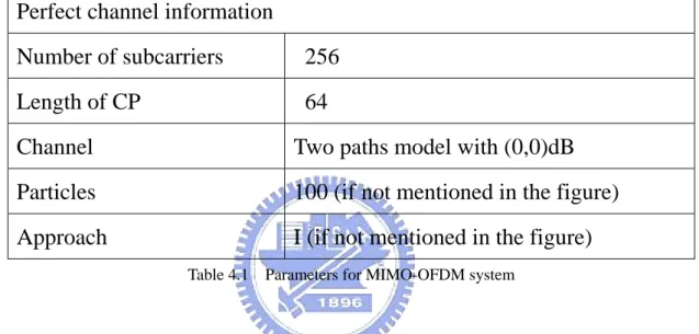
Chapter 4 Simulation results ... 37

4.1 Parameters for MIMO-OFDM spatial multiplexing system ... 37

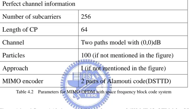
4.2 Parameters for MIMO-OFDM with Space frequency block code system ... 39

Chapter 5 Conclusion ... 53

List of Tables

Table 4.1 Parameters for MIMO-OFDM system ... 37  Table 4.2 Parameters for MIMO-OFDM with space frequency block code system ... 39 

List of Figures

Figure 2.1 Spatial multiplexing system ... 4 

Figure 2.2 Block diagram for error propagation mitigation method ... 23 

Figure 3.1 Transmitter structure for MIMO-OFDM with space frequency block code ... 26 

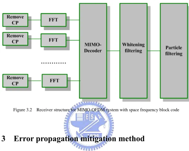
Figure 3.2 Receiver structure for MIMO-OFDM system with space frequency block code ... 33 

Figure 3.3 Block diagram for error propagation mitigation method in MIMO-OFDM with space frequency block code system ... 36 

Figure 4.1 MIMO-OFDM 4X4 QPSK modulation for different approaches ... 41 

Figure 4.2 MIMO-OFDM 6X6 QPSK modulation for different approaches ... 42 

Figure 4.3 MIMO_OFDM 4X4 QPSK for different detection schemes ... 43 

Figure 4.4 MIMO_OFDM 4X4 16 QAM for different detection schemes ... 44 

Figure 4.5 MIMO_OFDM 6X6 QPSK modulation with and without sorted QR decomposition ... 45 

Figure 4.6 MIMO-OFDM 6X6 QPSK with particles equal to 50 and 75 ... 46 

Figure 4.7 MIMO OFDM 6X6 16QAM modulation with and without sorted QR decomposition with approach I ... 47 

Figure 4.8 MIMO OFDM 6X6 16QAM modulation particles equal to 50,75 and 200 ... 48 

Figure 4.9 MIMO_OFDM 4X2 QPSK with space frequency block code for different detection scheme ... 49 

Figure 4.10 MIMO_OFDM 4X2 16QAM with space frequency block code ... 50 

Figure 4.11 MIMO_OFDM 4X4 QPSK with space frequency block code ... 51 

Chapter 1

Introduction

Multiple-input-multiple-output (MIMO) system gets a great interest in communication system because of its ability to increase the throughput under the same total amount of transmitting power compare with single-input-single-output (SISO) system. The main idea is to transmit signals using multiple transmitting antennas and receiving signals using multiple receiving antennas. The bandwidth efficient can be increased by using this technique.

1.1 MIMO system

MIMO technique is mainly divided into three categories. First category is called spatial multiplexing. Spatial multiplexing is a transmission technique in MIMO system to transmit data signals independent and separately from each of the multiple transmit antennas. Therefore, the space dimension is reused more than once. The capacity can be increased by this technique if the channel matrix is full rank. In [1], ‘BLAST (Bell Laboratories -Layered -Space-Time )’, is a typical technique for spatial multiplexing.

Second, known as beamforming system, is to form a beam pattern by designing the arrangement of antenna array. It has an improvement as compared with omni-directional transmission because it can select directional transmission so it has directivity gain. Power can be focused on a particular direction and can be diminished the inference of other signals or other users.

Final system is pre-coding system. This system utilizes coding technique that called space time block code to increase diversity. Space time block code are normally presents as orthogonal. This means that each column in the equivalent channel matrix is orthogonal to

other columns in the equivalent channel matrix. The decoding scheme for orthogonal space time block code is very simple, and easy to decode at the receiver side. Its disadvantage is that this system decreases the data rate as compared with spatial multiplexing in order to get diversity gain. Another scheme is proposed in space time block code is that such code is not orthogonal but it can achieve a higher data rate. Chapter three is focus on this scheme in order to get higher data rate.

1.2    MIMO‐OFDM system 

MIMO system can be used to increase the throughput in flat fading channel. Flat fading channel is a good condition for MIMO system. However, in MIMO system, channel may not be flat fading. Orthogonal frequency division multiplexing (OFDM) system can provide a flat fading condition for MIMO system and against ISI effect. Hence, MIMO system combining with OFDM system is frequently proposed for high data rate transmission scheme recently. On the other hand, especially in spatial multiplexing system, interference in MIMO-OFDM is more severe than in single input single output (SISO) OFDM system and the complexity of data detection in MIMO-OFDM system is higher than the complexity in SISO OFDM system. In BLAST system (spatial multiplexing), as proposed in [3], the system called VBLAST (Vertical-Bell Laboratories -Layered -Space-Time) system, is widely used in spatial multiplexing system for rich scattering communication environment because it has better performance and spectral efficiency as compared with spatial multiplexing system using conventional nulling method.

1.3 About the thesis

method in data detection in spatial multiplexing system. Then we describe two modified methods to mitigate the error propagation problem in particle filtering. Chapter 3 presents the use of particle filtering for data detection in MIMO-OFDM with space frequency block code system. Then also presents a method to mitigate the error propagation. Chapter 4 shows all the simulations for each detection scheme in both spatial multiplexing in MIMO-OFDM and MIMO-OFDM with space frequency block code system. Finally, conclusions are introduced in the last chapter.

Chapter 2

Data detection in MIMO-OFDM system with particle

filtering method

2.1 Spatial multiplexing system description:

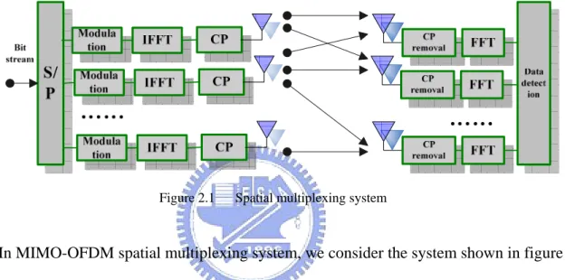
Figure 2.1 Spatial multiplexing system

In MIMO-OFDM spatial multiplexing system, we consider the system shown in figure 1. We assume that there are M transmitting antennas and N receiving antennas. At the

transmitter side, bit stream is divided into M data layers and mapped each data layer to be M modulated signal streams. M modulated signal streams in M layer pass through IFFT, add cyclic prefix and then transmit parallel through M transmitting antennas. At the receiver side, there are N receiving antennas, after cyclic prefix removal and pass through FFT, the received signal vector X can be expressed as

Tx

X = HS + N (2.1)

Where X is an N by 1 received signal vector, H is a N by M channel matrix, S is a M by 1 _Tx transmitted signal vector and N is a N by 1 noise vector. The channel matrix H is assumed to be full rank. The received signal vector is passed through the data detection scheme as shown in figure 1. There are several schemes for data detection in MIMO-OFDM BLAST system.

One of them is VBLAST- OSIC.

V-BLAST Zero-forcing OSIC [3] scheme is widely used in spatial multiplexing system. The procedure of the V-BLAST can be mainly divided into following steps: first, ordering the received signal according to signal to noise (SNR) ratio in descending order, then detects the first signal that belongs to the highest order of SNR. After detecting the first signal, then treats this signal as interference and cancelled out from the received signal vector, then starts to detect the second highest SNR signal. This process keeps moving until all the data are

detected. In spatial multiplexing system, the optimum solution is to use Maximum likelihood (ML) detection. However, ML detection is an exhaustive search, the complexity increases either the number of transmitting antennas or order of modulation increases.

On the other hand, Maximum a posteriori (MAP) detection also give an optimum solution, therefore, if we can obtain the posteriori pdf (probability density function) or pmf(probability mass function), then MAP detection can be used for data detection. MAP approach is as same as ML approach. As describes above, the received signals can be expressed as

Tx

X = HS + N , (2.2)

All the elements in vector X, H, S and N are complex number. In this thesis, we only _Tx consider the case that the number of transmitting antennas is equal to or less than the number of receiving antennas.

Assuming that the channel matrix H is full rank such that it can be decomposed using QR decomposition as shown below

H = QR, (2.3)

where R is an upper triangular matrix and Q is an orthogonal matrix.

Multiply QH (where ()Hdenoted as Hermitian of a matrix) to X and the system model can be expressed as

H

Tx

X = Q X = RS + N (2.4)

We consider the case that the number of transmitted antennas are equal to the received antennas(M=N), so that $ $ $ 1 ₁ 1 11 12 1 2 2 2 22 2 ... 0 .. ... ... . ... 0 0 .. ... ... ... . ... 0 0 .. 0 tx M tx M MM txM M _M n x s R R R s x n R R R s x n ⎡ ⎤ ⎡ ⎤ _{⎡ ⎤ ⎢ ⎥} ⎢ _{⎥ ⎡ ⎤ ⎢} ⎥ ⎢ ⎥ ⎢ _{⎥ ⎢ ⎥ ⎢} ⎥ ⎢ ⎥ ⎢ _{⎥ ⎢= ⎥ ⎢ ⎥+ ⎢ ⎥} ⎢ _{⎥ ⎢ ⎥ ⎢ ⎥ ⎢ ⎥} ⎢ _{⎥ ⎢ ⎥ ⎢ ⎥ ⎢ ⎥} ⎢ ⎥ ⎣ _{⎦ ⎢ ⎥} ⎣ ⎦ ⎢ ⎥ ⎢ ⎥ ⎣ ⎦ ⎣ ⎦ (2.5)

We re-define some parameters, first of all, we define three vectors Y, S and n as the reverse order of X ,S and N where _Tx

$ $1 2 $ 1 $ 1 2 1 [y_M, ,....y_M− y y, ]T [ , x x ,....xM− ,xM] T , = = Y 1 1 1 1 [s_M, s_M−,.... ]s T [s_tx , ....,s_txM−,s_txM] andT = = S $ $1 2 $ 1 $ 1 1 [n_M,n_M−,.... ] = [ , n n n ,....nM−,nM]T = n

The new expression can be shown as

11 12 1 1 1 1 22 2 1 1 1 ... 0 .. ... . ... ... 0 0 .. ... ... . ... ... 0 0 .. 0 M M M M M M M M MM y s n R R R y s n R R R y s n − − − ⎡ ⎤ ⎡ ⎤ ⎡ ⎤ ⎡ ⎤ ⎢ ⎥ ⎢ ⎥ ⎢ ⎥ ⎢ ⎥ ⎢ ⎥ ⎢ ⎥ ⎢ ⎥ ⎢ ⎥ ⎢ ⎥= ⎢ ⎥ ⎢+ ⎥ ⎢ ⎥ ⎢ ⎥ ⎢ ⎥ ⎢ ⎥ ⎢ ⎥ ⎢ ⎥ _{⎣ ⎦}⎢ ⎥ ⎢ ⎥ ⎢ ⎥ ⎢ ⎥ ⎢ ⎥ ⎣ ⎦ ⎣ ⎦ ⎣ ⎦ (2.6)

Where

y

_k,s_kand n_krepresent th

k element of vector Y, S and n.

The relationship between

y

_k and vector S is

y

k

=

h s

k

(

_1:k

)

+

nk where

s

_1:k=[ ... ]s s_{1 2} sk .

Our goal is to find a scheme to detect the data sequence

s

_1:M=[ ... ]s s_{1 2} s_M .

2.2 MAP decision:

obtain the posteriori distribution and assume that each entry in the noise vector is independent Gaussian distribution, zero mean and varianceσ . 2

The posteriori distribution will be expressed as:

1: 1: / 2 2 / 2 2 1 1 ( | ) exp( ( ) ( )) (2 ) ( ) 2 M M M M p s y π σ σ = − _{Y HS}− H _{Y HS (2.7)} − Where S = s_1:M and Y = y_1:M, H is the M by M channel matrix.

The MAP decision becomes

1: 1: / 2 2 / 2 2 1 1 ( | ) exp( ( ) ( )) (2 ) ( ) 2 M M M M p s y π σ σ = − _{Y HS}− H _{Y HS (2.8)} − S A arg min ( ) ( ) ∈ ⇒ _{Y HS}− H _{Y HS (2.9)} − 2 S A arg min ∈ ⇒ Y HS− (2.10) From equation (2.10), MAP decision needs to test all the possible combinations and choose the minimum distances. The complexity is related to two factors: first, the modulation scheme, for example, QPSK, 16QAM, and second, the number of transmitting antennas. The

complexity increases exponentially as one of the factors increases. So that the complexity is O(A ), where M is the number of transmitting antennas and A is the modulation scheme. For M example, QPSK with 4 transmitting antennas, number of trials will become 4

4 =256.

Furthermore, if modulation change to 16QAM, number of trials will become 164 =65536. MAP decision is not practical in this case.

2.3 Monte Carlo method

Before we mention the detail of particle filtering or called sequential Monte Carlo method algorithm, first we take a look on how a posteriori distribution can be approximated by a set of random samples.

p s( _1:M =s1:M |y_1:M)=

∫

p s( _1:M |y_1:M) (δ s_1:M −s1:M)ds_1:M (2.11)

If Np is large and then the desired posteriori distribution can be approximated as :

( ) 1: 1: 1: 1: 1: 1 1 ( | ) ( ) Np i M M M M M i p s s y s s Np = δ = ≈

∑

− (2.12) ( ) 1: 1: ( ) 1: _1: ( ) 1: 1: 1 when ( ) 0 when i M M i M _M i M M s s where s s s s δ − _{= ⎨}⎧⎪ = ⎫⎪_⎬ ≠ ⎪ ⎪ ⎩ ⎭ (2.13) As the equation mentioned above,

1: 1

{ }

k

i Np i

s ₌ denoted a set of samples drawn from a desired

posteriori distribution function, the posteriori distribution function can be approximated by

( ) 1: 1: 1: 1: 1 1 ( | ) ( ) Np i M M M M i p s y s s Np = δ ≈

∑

− (2.14) Monte Carlo approach is one of the methods to construct the approximation of high

dimensional posteriori distribution. If we can draw samples directly from the desired

posteriori distribution p s( _1:M |y_1:M), so that the posteriori distribution can be constructed by

all the samples 1:

( ) 1

{ M}

i Np i

s ₌ (where Np represents the number of samples) drawn from the desired

posteriori distribution and this approximation will converge to the true posteriori distribution as there are infinite number of samples.

2.4 Importance sampling

Importance sampling is a method to approximate the desired posteriori distribution by drawing samples {s( )i }_iNp₌₁ from a trial function called importance distribution q s( _1:M |y_1:M) if

the desired posteriori distribution cannot be drawn directly. This importance distribution is tractable for sampling. The different between Monte Carlo method and importance sampling is that importance sampling needs to compute the weights of the corresponding i th sample

using ( ) ( ) 1: ( ) 1: ( | ) ( | ) i i k i k p w q = s y s y .

The approximation of the posteriori distribution can be derived as :

1: 1: 1: 1: 1: 1: 1: 1: ( _M M | _M) ( _M | _M) ( _M M) _M p s =s y =

∫

p s y δ s −s ds (2.15) 1: 1: 1: 1: 1: 1: 1: 1: 1: 1: 1: 1: 1: 1: ( | ) ( | ) ( | ) ( ) ( w( ) = ) ( | ) ( | ) M M M M M M M M M M M M M M p s y p s y q s y s s ds define s q s y δ q s y =

∫

− (2.16) 1: 1: 1: 1: 1: 1: 1: 1: 1: 1: 1: 1: 1: 1: w( ) ( | ) ( ) (Since w( ) ( | ) = 1) w( ) ( | ) M M M M M M M M M M M M M M s q s y s s ds s q s y ds s q s y ds δ − =

∫

∫

∫

(2.17)

If Np is large and then the posteriori distribution can be approximated as : (1/Np) ≈ ( ) ( ) 1: 1: 1 ( ) (1/ ) Np i i M M M i w s s Np δ = −

∑

( ) ( ) 1: 1: ( ) 1 1 1 (1/ ) ( ) (where W = ) (2.18) Np N i i i M M M M Np i i i M i W w s s w w δ = = = =

∑

−

∑

∑

( ) ( ) 1: 1: ( ) ( ) 1: 1: 1: 1: _{( )} ( ) 1: 1: 1: 1: 1 when ( | ) ( ) and ( | ) 0 when i i M M i i M M M M _i M i M M M M s s p s y where s s w q s y s s δ − =⎧⎪_⎨ = ⎫⎪_⎬ = ≠ ⎪ ⎪ ⎩ ⎭ (2.19) Defined ( ) ( ) ( ) 1 i i Np i i w w w = =

∑

as normalized weight corresponding to i th sample, then the posteriori

distribution can be approximated as

( ) ( ) 1: 1: 1: 1: 1 ( | ) ( ) Np _i i M M M M i p s y w δ s s = ≈

∑

− . (2.20) The importance distribution can be chosen freely, however, the variance will be

increased if the importance function is not highly related to the true posteriori distribution.

2.5 Particle filtering Methods [4]

If we need to draw samples directly from the posteriori distribution, we need to know the joint posteriori distribution first. The complexity is same as or higher than MAP decision. Now, if we do not have any information about the desired posteriori distribution, however, we have the conditional probability distribution p(y | s ) , particle filtering or called sequential _{k 1:k}

monte carlo method described in [5] and [6] provides a new method to obtain the posteriori distribution with low complexity by using the idea of importance sampling. The main idea is to estimate the desired posteriori distribution by drawing a set of random samples from importance distribution and to update the corresponding weights recursively.

Let’s take a look on how all the samples can be drawn recursively. After finishingk−1th

tracking, we have samples

{ }

_1:( ) ₁

1 Np i

k− _i=

s drawn from q(s_1:k−1|y_1:k−1)and weights

(i) ( ) ( )

k-1 1: 1 1: 1 1: 1 1: 1

w = p s( i_k− |y _k− ) / (q si_k− |y _k−) ,where I = 1 : Np. Furthermore, the importance

distribution q s( _1:k |y_1:k) can be factorized as two components such that

1: 1: 1: 1 1: 1: 1 1: 1

( _k | _k) ( _k | _k , _k) ( _k | _k )

q s y =q s s ₋ y q s ₋ y ₋

(2.21) Which means that we can obtain Np sampled sequences(from 1 to k)

{ }

_1:( )

1 Np i

k _i=

s from

importance distribution q s( _1:k|y_1:k) by sampling Np sampled sequences with length k-1(from

1 to k-1 )

{ }

( ) 1: 1 ₁

Np i

k− _i=

s from q(s_1:k−1|y_1:k−1) and by sampling a new set of samples

{ }

( ) 1 Np i k _i=

s

from q(s s_k| _1:k−1,y_1:k). The weight update equation is

( ) ( ) 1: 1: ( ) 1: 1: ( | ) ( | ) i i k k k i k k p s y w q s y = (2.22) ( ) ( ) 1: 1: 1 1: 1: 1 1: 1 ( ) ( ) ( ) 1: 1: 1 1: 1: 1 1: 1 ( | , ) ( | ) ( ) ( ) ( | , ) ( | ) i i k k k k k k i i i k k k k k k p y s y p s y p y p y q s s y q s y − − − − − − = (2.23) ( ) ( ) ( ) 1: 1: 1 1: 1 1: 1 ( _k| i_k) ( _ki ) ( i_k | _k ) ( _k ) p y s p s p s ₋ y ₋ p y ₋ = 1: 1 1: 1 ( _k| _k ) ( _k ) p y y ₋ p y ₋ q s( _k|s_1:( )i_k−1,y_1:k) (q s_1:( )i_k−1|y_1:k−1) (2.24) ( ) ( ) ( ) 1: 1 1: 1 1: ( ) ( ) ( ) 1: 1 1: 1 1: 1 1: ( | ) ( | ) ( ) * ( | ) ( | , )

ik k k ik ki i i i k k k k k p s y p y s p s q s y q s s y − − − − −

∝

(2.25) ( ) ( ) ( ) 1: 1 ( ) ( ) 1: 1 1: ( | ) ( ) = ( | , ) i i i k k k k i i k k k p y s p s w q s s y − − (2.26)

The posteriori distribution can be approximated using

{ }

_1:( )

1 Np i

k _i=

s recursively as equation (2.21) and updated weights{w_k( )i₋₁}Np_i=1 recursively using equation (2.26), then normalize all the

( ) ( ) 1: 1: 1: 1: 1 ( | ) ( ) Np _i i k k k k k i p s y w δ s s = ≈

∑

− (2.27) Since it is an approximation method, increasing the number of samples will increase the accuracy of the approximation. In the jargon of particle filtering, these samples in each tracking are called particles.

The problem is how to choose the importance distributionq(s s_k | _1:k−1,y_1:k). In [7], it is mentioned, in order to minimize the variance of the approximation, the importance function is chosen as: ( ) ( ) 1: 1 1: 1: 1 1: ( | i , ) ( | i , ) k k k k k k q s s ₋ y = p s s ₋ y (2.28)

If we choose the importance function as equation (2.28),

1: 1 ( ) ( ) 1: ( | , ) k i i k k p s s ₋ y can be factorize as 1: 1 1: 1 1: 1 1: 1 1: 1 ( ) ( ) ( ) ( ) ( ) 1: 1: 1 ( ) ( ) 1: ( ) ( ) 1: ( | , ) ( | ) ( ) ( | , ) ( | ) ( ) k k k k k i i i i i k k k k i i k k i i k p y s s p s s p s p s s y p y s p s − − − − − − = (2.29) ( ) ( ) ( ) 1: 1 1: 1 1: 1 ( _k| _ki , i_k ) ( _k | i_k ) p y s s ₋ p y ₋ s ₋ = ( ) ( ) 1: 1 ( _ki ) ( i_k ) p s p s ₋ ( ) ( ) 1: 1 1: 1 1: 1 ( _k| i_k ) ( _k | i_k ) p y s ₋ p y ₋ s ₋ p s( _1:( )i_k−1) (2.30) ( ) ( ) 1: ( ) 1: 1 ( | ) ( ) = ( | ) i i k k k i k k p y s p s p y s ₋ (2.31) Substitute ( ) ( ) ( ) ( ) 1: 1: 1 1: 1: 1 1: ( ) 1: 1 ( | ) ( ) ( | , ) ( | , ) = ( | ) i i i i k k k k k k k k k i k k p y s p s q s s y p s s y p y s − − −

= into equation (2.26), the

weight updated equation is

( ) ( ) ( ) ( ) 1: 1 ( ) ( ) 1: 1 1: ( | ) ( ) ( | , ) k i i i i k k k k k i i k k p y s p s w w q s s y − − ∝ (2.32) ( ) 1: ( ) 1 ( _k| i_k) i k p y s w₋ ∝ ( ) ( _ki ) p s _1:( )₁ ( ) 1: ( | ) ( | ) i k k i k k p y s p y s − ( ) ( _ki ) p s (2.33) ( ) ( ) 1 1: 1 i ( | i ) k k k w₋ p y s ₋ = (2.34) ( ) ( ) 1 ( | , 1: 1) ( )

=

k i i k k k k k s w ₋

∑

p y s s ₋ p s (2.35) The term p y( _k|y_1:k−1) can be ignored because it is not affected the approximation of k th tracking after normalization. From the deviation of equation (2.35), we can observe that the

weight in i th particle at k th tracking depends on two factors: The previous weights of i th particle at k-1 th tracking and a new term ( | , _1:( )₁) ( )

k

i

k k k k s

p y s s ₋ p s

∑

. Suppose that we have Np

particles from 1 : k-1 which denoted as {s_1:( )i_k−₁}_iNp=₁ and Np weights from k-1 which denoted as

( ) 1 1

{w_ki−}_iNp= .Then the new particles can be drawn from the importance distribution

( ) ( )

1: 1 1: 1: 1 1:

( _k | i_k , _k) ( _k| i_k , _k)

q s s − y = p s s − y and then update the corresponding weight using equation

(2.35). After that normalize all the weights at M th tracking by

( ) ( ) ( ) 1 i i M M _Np i M i w w w = =

∑

. In the jargon of

particle filtering, this procedure is called Sequential importance sampling (SIS) scheme. The procedure of k th tracking is summarized as following:

－For i = 1 to Np

◆ Draw a particle from the importance distribution (2.28) ◆ Calculate the weight by using equation(2.35)

◆ Store the new particle ( )i k

s to s_1:( )i_k−1 －End For

◆ Normalized all the weights

2.6    Degeneracy 

After several tracking, the variance of the estimator will increases as shown in [7], since some of the particles have negligible weights and do not have any contribution to the process. This problem is called degeneracy. In [10], resampling algorithm is used to overcome this problem. The main idea is to replace some small weighted samples by some large weighted samples. In [8] and [9]. Both papers mention that one of the methods to measure degeneracy is to calculate the effective sample size N_eff . N_eff can be obtained by

( ) 2 1 1 ( ) eff Np _i k i N w = =

∑

. (2.36)

So that we can set a threshold sample size called Ns. Ns is set as 60% of Np in our simulation. If N_eff <Ns, resampling algorithm is needed.

Algorithm for resampling „ For i = 1 to Np

Generate a random variable U with uniform distribution from [0 1] For j = 1 to Np

( ) ( ) ( )

_ _ki _ _ki _kj

w new =w new +w (2.37)

If w new >U , then _ _k( )i s new_ _k( )i = $ (2.38) s( )kj

Break; End For ( )i 1 k w Np = (2.39) End For

After resampling, new set of particles are obtained, the connection with previous samples is broken and their weights at k th tracking are all equal. In the jargon of particle filtering, this procedure is called Sequential importance sampling (SIS) with resampling scheme.

The procedure of k th tracking is summarized as following: －For i = 1 to Np

◆ Draw a particle from the importance distribution from equation (2.28) ◆ Calculate the weight by using equation (2.35)

◆ Store the new particle ( )i k

s to s_1:( )i_k−₁

－End For

◆ Normalized all the weights by using

( ) ( ) ( ) 1 i i k k _Np i k i w w w = =

∑

◆ Calculate the effective sample size N_eff using (2.36)

◆ If N_eff < Ns , then do the resampling scheme.

2.7    Data detection scheme in MIMO-OFDM BLAST

system with particle filtering:

In MIMO-OFDM spatial multiplexing system, we assume that the channel matrix H is full rank such that it can be decomposed using QR decomposition as shown H = QR and

H

Tx

X = Q X = RS + N (2.40) Since R is an upper triangular matrix, one of the methods for data detection is to use decision feedback method that detects signals from the bottom to the top.

First, compute the probability of (p s_txM |y_M). For example, the distribution of noise in each

entry is complex Gaussian distribution then detection s_txM using minimum distance. The

next step is to compute p s( _txM−1|s_txM,y_M−1) and detects_txM−1. The process keeps moving until

all the signals are detected. However, this method has error propagation problem and the SNR of each signal mainly depends on the diagonal. On the other hand, since QH is an

orthogonal matrix, so that after multiplying QH to the initial noise vector, the new noise vector is also independent white noise vector. As mentioned in section 2.1, we define three new vectors Y, S and n, and the relationship between y is also dependent on _k s and _1:k n _k

which is y_k =R s_{k k k,} +R_{k k,} +₁s_k−₁+...R_{k M,} s₁+ . We assume that the noise before multiplying n_k

H

Q to the received signal vector is white noise. Hence, after multiplying QHto the received signal vector, the noise vector is still a white noise vector. We treat each noise entry n as an _k

( ) 1: 1 1:

( _{k k} | i_k , _k)

p s =a s ₋ y which can be factorized as

1: 1 1: 1 1: 1 1: 1 1: 1 ( ) ( ) ( ) 1: 1: 1 ( ) 1: ( ) ( ) 1: ( | , ) ( | ) ( ) ( | , ) ( | ) ( ) k k k k k i i i k k k k k k i k k k i i k p y s a s p s a s p s p s a s y p y s p s − − − − − − = = = = (2.41) ( ) ( ) 1: 1 1: 1 ( ) 1: 1 ( | , ) ( ) ( | , ) ( ) = = ( | ) i i k k k k k k k k k k i k k p y s a s p s p y s a s p s p y s − − − = = ( ) 1: 1 ( _k | _k, i_k ) ( )_k p y s s ₋ p s

∑

(2.42)

We can observe that the first term in numerator p y( _k|s s_k, _1:( )i_k−1) is a Gaussian distribution

which mean is equal to y_k −R a_{k k, k} −R_{k k,} +₁s_k−₁−...R_{k M,} s₁(wherea is one of the signal points k

in signal constellation) and variance is equal toσ2

and the second term in numerator is assumed to be equally likely. Finally, we can draw samples from p s( _k |s_1:( )i_k−₁,y_1:k)which is

equal to equation (2.36). For example, in QPSK modulation, the set of $a is {M

1 (1 ) 2 + ,-j 1 ( 1 ) 2 − + ,j 1 ( 1 ) 2 − − ,j 1 (1 )

2 − } also there is 16 combinations for 16-QAM modulation. j For example, for the QPSK modulation, the particle filtering (SIS) is shown below:

In k-th tracking:

－For i = 1 to Np

◆ Draw samples from importance distribution p s( _k|s_1:( )i_k−1,y_1:k)

( ) ( ) 1: 1 1: 1 1: ( ) 1: 1 ( ) 2 1: 1 , , 1 1 , 1 ( | , ) Where ( | , ) ( | , ) since ( | , ) = ( ... , ) k i i k k k k k k k i k k k k s i k k k k k k k k k k k k M p y s a s p s s y p y s a s p y s a s N y R a R s R s σ − − − − + − = = = = − − −

∑

( ) 1: 1 1 1 ( | (1 ), ) 2 i k k k p y s = + j s ₋ = , β ( | 1 ( 1 ), _1:( )₁) ₂ 2 i k k k p y s = − + j s ₋ =β , ( ) 1: 1 3 1 | ( 1 ), ) 2 i k k k py s = − − j s ₋ =β , ( | 1 (1 ), _1:( )₁) ₄ 2 i k k k p y s = − j s ₋ =β And ( ) 1 1 1: 1 1: 1 2 3 4 1 ( (1 ) | , ) 2 i k k k p s j s y β α β β β β − = = + = + + + ,

( ) 2 2 1: 1 1: 1 2 3 4 1 ( ( 1 ) | , ) 2 i k k k p s j s y β α β β β β − = = − + = + + + ( ) 3 3 1: 1 1: 1 2 3 4 1 ( ( 1 ) | , ) 2 i k k k p s j s y β α β β β β − = = − − = + + + , ( ) 4 4 1: 1 1: 1 2 3 4 1 ( (1 ) | , ) 2 i k k k p s j s y β α β β β β − = = − = + + +

Generate a uniform distribution U between [0 ,1] If α₁>U > 0, then ( ) 1 (1 ) 2 i k s = + , j If α₁+α₂>U >α₁, then ( ) 1 ( 1 ) 2 i k s = − + j If α₁+α₂+α₃>U>α₁+α₂, then ( ) 1 ( 1 ) 2 i k s = − − , j If 1>U>α₁+α₂+α₃ then ( ) 1 (1 ) 2 i k s = − j

◆ Update the weight using ( ) ( ) ( ) ( )

1 ( | , 1: 1) ( ) k i i i i k k k k k k s w =w₋

∑

p y s s ₋ p s Sincep y( _k|s_k =a_M,s_1:( )i_k−1)=β_M, hence ( ) ( ) 1 2 3 4 1 ( ) 4 i i k k w =w₋ β β+ +β +β .

◆ Store the new particle ( )i k

s to s_1:( )i_k−1 －End For

If k = M

◆ Normalized all the weights by using

( ) ( ) ( ) 1 i i M M _Np i M i w w w = =

∑

.

Example : For MIMO-OFDM 4X4 system with BPSK modulation. After QR decomposition, the signal model become

4 11 12 13 14 4 4 3 22 23 24 3 3 2 33 34 2 2 1 44 1 1 0 0 0 0 0 0 y R R R R s n y R R R s n y R R s n y R s n ⎡ ⎤ ⎡ ⎤ ⎡ ⎤ ⎡ ⎤ ⎢ ⎥ ⎢ ⎥ ⎢ ⎥ ⎢ ⎥ ⎢ ⎥ ⎢₌ ⎥ ⎢ ⎥ ⎢ ⎥₊ ⎢ ⎥ ⎢ ⎥ ⎢ ⎥ ⎢ ⎥ ⎢ ⎥ ⎢ ⎥ ⎢ ⎥ ⎢ ⎥ ⎣ ⎦ ⎣ ⎦ ⎣ ⎦ ⎣ ⎦ (2.43)

In order to draw particles for s , first of all, calculate the probability for ₁

1 1 1 1 1 1 ( | 1 ) ( | 1 ) ( | 1 ) p y s p y s p y s = = + = − and _{1 1} 1 1 _{1 1} ( | 1 ) ( | 1 ) ( | 1 ) p y s p y s p y s = −

two probabilities. For example, assume that 1 1 1 1 1 1 ( | 1 ) ( | 1 ) ( | 1 ) p y s p y s p y s = = + = − = 0.6 , 1 1 1 1 1 1 ( | 1 ) ( | 1 ) ( | 1 ) p y s p y s p y s = −

= + = − = 0.4 and draw 5 particles, we generate 5 random variables

with uniform distribution(U1 to U5) between [0 1 ]. For particle i, if Ui <0.6, s₁( )i is

1,otherwise, s₁( )i is -1. The normalized weight for all particles i = 1 to 5 are w = 1/5 for the ₁( )i

first tracking. Assuming that the five particles are {1 1 1 -1 -1}. In order to draw particles for

the second tracking s₂( )i , first calculate the

( ) 2 2 1 ( ) ( ) 2 2 1 2 2 1 ( | 1, ) ( | 1, ) ( | 1, ) i i i p y s s p y s s p y s s = = + = − and ( ) 2 2 1 ( ) ( ) 2 2 1 2 2 1 ( | 1, ) ( | 1, ) ( | 1, ) i i i p y s s p y s s p y s s = −

= + = − , i.e., for 2nd particle in 2nd tracking, since

(2) 1 s = 1, calculate (2) 2 2 1 (2) (2) 2 2 1 2 2 1 ( | 1, 1) ( | 1, 1) ( | 1, 1) p y s s p y s s p y s s = = = = + = − = (assume it is 0.3) and (2) 2 2 1 (2) (2) 2 2 1 2 2 1 ( | 1, 1) ( | 1, 1) ( | 1, 1) p y s s p y s s p y s s = − =

= = + = − = (assume it is 0.7) and generate a uniform

random variable U, if U<0.3, then s₂(2)=1 ,otherwise s₂(2)=-1 ,and the corresponding weight for 2nd particle for 2nd tracking is

( 2) ( 2) ( 2) ( 2) 2 2 1 2 2 1 2 1 ( ( | 1, 1) ( | 1, 1)) 2 p y s s p y s s w =w = = + = − = ,

From the equation shown above, we observe that the i th particle at 2 th tracking is related to the previous i th particle and weight. After getting five new particles and update five corresponding weights for i th particle at 2nd tracking. Assume that they are {-1 -1 -1 -1 1}, attach these five particles to the first five particles, we can get

1 1 1 1 1 -1 -1 -1 -1 1 − − ⎧ ⎫ ⎨ ⎬

⎩ ⎭ ,the first row represents the first tracking particles(

( ) 1

i

s ) and second

2nd tracking is w₂(1:5) = {0.3 0.3 0.3 0.05 0.05}. Keep moving until 4th tracking is done. We can get 1 1 1 1 1 -1 -1 -1 -1 1 1 1 1 1 1 1 1 1 1 1 − − ⎧ ⎫ ⎪ ⎪ ⎪ ⎪ ⎨ ⎬ ⎪ ⎪ ⎪ _{− −} ⎪ ⎩ ⎭ and w₄(1:5)={0.25, 0.25, 0.25 0.05 0.2 }

First, consider the first three columns, we discover that the first three columns are identical to each other which is s_1:4( )i = {1 -1 1 1}, the 4th and 5th column are different to the first 3 columns, they are s_1:4(4)= {-1 1 -1 1} and s_1:4(5)= {-1 1 1 -1}. The posteriori distribution can be

approximated as:

1:4 1:4 1:4 1:4 1:4

( | ) 0.75* ( {1 -1 1 1}) 0.05* ( {-1 1 -1 1}) 0.2* ( {-1 1 1 -1})

p s y ≈ δ s − + δ s − + δ s −

The data is the reverse order of stx1:4=[ ]s s s s4 3 2 1 _{and the histogram can be plotted as}

2.8 Detection Scheme

Approach I : Sequence detection

1: 1: arg max ( _1: | _1: ) M M _{M M} s s = p s y $ _(2.44) This process needs to find all the same sequences and adds all the weights which belong to the same sequence This process will increase the complexity if the sequence is too long, which means that if the number of tracking increases, the complexity will increases.

Approach II : Detect directly from the marginal posteriori probability

( ) ( ) 1: 1 ( | ) ( ) Np _i i k k k k k i p s y w δ s s = ≈

∑

− (2.45)

the detection scheme needs to find one dimension only. The searching process is to sort all the signals which belong to the same constellation and to add all the weights which belong to the same signal. The detection scheme after sorting and adding all the weights is shown as

arg max ( | 1: ) k k _{k k} s s = p s y $ _(2.46)

Approach III : Find the expectation value from the marginal posteriori distribution s$k ( ) ( ) 1: 1 [ | ] Np _i i k _{k k} k _k i s E s y w s = =

∑

$ _(2.47)

As the equation shown above, no sorting is needed. However, Multiplications are needed for this approach. The performance will have same degradation for using approach II and III for data detection.

2.9 Error mitigation method

For approach II and III, one of the problems using particle filtering for data detection in spatial multiplexing is the error propagation problem. If the particles in previous tracings did not draw well, the estimated posterior distribution will be affected by error sampling. We can see that the top signal will be affected by all the other signals. Data detection using approach II and III for the top signal will has the worst performance as compared with other signals. We proposed a modified method for data detection in spatial multiplexing system with particle filtering. First, we consider the channel matrix and review the complex value problem of Gram-Schmidt algorithm for QR decomposition. Assume that all the entries in channel H are complex and consider the case that the number of transmitting antennas M is equal to the number of received antennas N (Assume that M=N), the channel matrix is shown as

[ .... .... ]

= _{1 2 M}

H h h h (2.48) Gram Schmidt process is

Step 1 : ₁ 1 1 h q = h (2.49) Step 2 : For n = 2 : M 1 1 1 1 ( ( ) ) / ( ( ) ) n n i i − − = = =

∑

H

∑

H n n i n i n i n i q h - q h q h - q h q (2.50) End For Step 3 : 2 2 2 2 2 3 3 .... ... 0 ... ... [ .... ... ] 0 0 .... . 0 0 0 .... . 0 0 0 0 ⎡ ⎤ ⎢ ⎥ ⎢ ⎥ ⎢ ⎥ ⎢ ⎥ ⎢ ⎥ ⎢ ⎥ ⎣ ⎦ H H H 1 1 1 1 M H H M H 1 M H n M q h q h q h q h q h H = q q q q h q h , (2.51)

On the other hand, we implement the Gram-Schmidt QR decomposition in reverse order as:

Step 1 : ₁ M M h q = h (2.52) Step 2 : For n = 2 : M $ $ $ $ $ 1 1 1 1 ( ( * ) ) / ( ( * ) ) n n i i − − = = = _M-n+1

∑

H _{M-n+1 M-n+1}

∑

H _M-n+1 n i i i i q h - q h q h - q h q (2.53) End For

A new orthogonal matrix is obtained which is Q = $₂ [q₁ q$₂ .... ... q$_M]. All the column vectors in channel matrix can be expressed as following:

The new QR expression is

$ $ $ $ $ $ $ $ $ $ 1 2 1 1 1 1 2 2 2 1 1 2 2 1 1 ) ) ) ) ) 0 [ ... .... ] [ .. .. ] 0 0 ) 0 0 0 ) 0 0 0 0 M M − − ⎡ ⎤ ⎢ ⎥ ⎢ ⎥ ⎢ ⎥ = ⎢ ⎥ ⎢ ⎥ ⎢ ⎥ ⎢ ⎥ ⎢ ⎥ ⎣ ⎦ H H H M H H M M 1 M H H (q h (q h ... ... (q h (q h (q h ... ... h h h q q q ... .... ... ... (q h (q h (2.54)

$ $ $ $ $ $ $ 1 2 1 1 1 1 2 2 2 2 1 1 ) ) ) ) ) 0 0 0 ) 0 0 0 ) 0 0 0 0 M M − ⎡ ⎤ ⎢ ⎥ ⎢ ⎥ ⎢ ⎥ ⎢ ⎥ ⎢ ⎥ ⎢ ⎥ ⎢ ⎥ ⎢ ⎥ ⎣ ⎦ H H H M H H 2 H H (q h (q h ... ... (q h (q h (q h ... ... R = ... .... ... ... (q h (q h

, so that channel matrix can be expressed as

another form of QR decomposition.

From the discussion above, we get two forms of QR decomposition which are

1 1 1 2 1 2 2 2 2 3 3 .... ... 0 ... ... [ .... ... ] 0 0 .... . 0 0 0 .... . 0 0 0 0 ⎡ ⎤ ⎢ ⎥ ⎢ ⎥ ⎢ ⎥ = ⎢ ⎥ ⎢ ⎥ ⎢ ⎥ ⎣ ⎦ H H H M H H M H 1 1 1 N H N M q h q h q h q h q h H = Q R q q q q h q h , (2.55) and $ $ $ $ $ $ $ $ $ $ 1 2 1 1 1 1 2 2 2 2 2 2 2 1 1 ) ) ) ) ) 0 [ .... ... ] 0 0 ) 0 0 0 ) 0 0 0 0 M M − ⎡ ⎤ ⎢ ⎥ ⎢ ⎥ ⎢ ⎥ = ⎢ ⎥ ⎢ ⎥ ⎢ ⎥ ⎢ ⎥ ⎢ ⎥ ⎣ ⎦ H H H M H H 1 N H H (q h (q h ... ... (q h (q h (q h ... ... H = Q R q q q ... .... ... ... (q h (q h (2.56)

The received vector passes through Q and ₁H Q matrix are ₂H

$ $ $ $ $ $ $ $ $ $ $ $ $ $ 1 2 1 1 1 1 2 ₂ 2 2 1 1 3 3 ) ) .... ... ) 0 ) ... ... ) .. 0 0 ) .... . .. 0 0 0 .... . 0 0 0 0 ) tx tx txM s s s ⎡ ⎤ ⎡ ⎤ ⎢ ⎥ ⎢ ⎥ ⎢ ⎥ ⎢ ⎥ ⎢ ⎥ ⎢ ⎥ + ⎢ ⎥ ⎢ ⎥ ⎢ ⎥ ⎢ ⎥ ⎢ ⎥ ⎢ ⎥ ⎢ _{⎥ ⎣ ⎦} ⎢ ⎥ ⎣ ⎦ H H H N H H N H H 1 1 1 Tx H N N (q h (q h (q h (q h (q h Y = Q X = R S + N = _{(q h} N (q h (2.57) and

$ $ $ $ $ $ $ $ $ $ $ $ 1 1 1 1 1 ₁ 2 1 2 2 2 2 ) ) ) ) ) 0 .. 0 0 .. 0 0 0 ) 0 0 0 0 tx tx txM s s s − − ⎡ ⎤ ⎡ ⎤ ⎢ ⎥ ⎢ ⎥ ⎢ ⎥ ⎢ ⎥ ⎢ ⎥ ⎢ ⎥ + ⎢ ⎥ ⎢ ⎥ ⎢ ⎥ ⎢ ⎥ ⎢ ⎥ ⎢ ⎥ ⎢ _{⎥ ⎣} ⎦ ⎣ ⎦ H H H N N H H N N H 2 2 2 Tx H N N (q h (q h ... ... (q h (q h (q h ... ... Y = Q X = R S + N = _{... .... ...} N ... .... (q h (2.58)

We observe from two equations shown above. In equation (2.57), we can use particle filtering, draw particles from the bottom signal to the top and use approach III to find the expectation value for each entry in the signal vector. On the other hand, in equation (2.58), we can use particle filtering method, draw particles from top to bottom and use approach III to find the expectation value for each entry in signal vector. Finally, we average two results, error propagation can be mitigated.

Block diagram for error propagation mitigation method

2.10 Sorted QR decomposition method

In [11], it is mentioned a method for sorted QR decomposition, which is similar to Gram- Schmidt algorithm. The idea of this method is to re-order the columns of channel matrix H for each orthogonal base searching. For Gram- Schmidt QR decomposition, we decompose the channel matrix H as shown in equation (2.55). Data detection by QR decomposition using particle filtering with approach II or III, as described before, the top signal will be affected by all the other signals. If particles in the previous stages did not draw well, the next stage signal samples will be affected by the previous stage samples. So that we need a large number of samples in order to obtain a much reliable posteriori probability. Sorted QR decomposition can improve such situation. The sorted QR decomposition combine with particle filtering use fewer particles to obtain a better performance compare with ordinary Gram Schmidt

decomposition as shown in simulations. The idea of sorted QR decomposition is to maximize the diagonal entry of channel matrix H from M to 1 by using a permutation vector p (where M is the number of transmitting antennas), such that minimizing the diagonal elements in each decomposition step in order to maximize the diagonal element in the subsequent steps. The algorithm is shown as:

Step 1 : Let R = 0; Q = H ; p = 1 ,2,..M Step 2 : For i = 1 to M

k = column of ( k 2

k = 1,..M

arg min q

) (2.59) Exchange columns i to k for Q , R and p

r_{i i,} = q (2.60) _i

q_i =q_i/r_{i i,} (2.61) For j = i+1 to M

q_j =q_j−r_{i j,} q_i (2.63) End

End

Where (M is the number of transmitting antenna , q is the lth column of orthogonal matrix _l

Q, r is the (i,j) entry of the upper triangular matrix R ) _{i j,}

The procedure of MIMO-OFDM system with particle

filtering and SQR decomposition

Step 1 : Using sorted QR algorithm to obtain matrix Q, R and p. Step 2 : Multiply Q to the received signal vector. H

Step 3:

For k = 1 to M (Where M is the number of transmitting antenna) For i = 1 to Np (Where Np is number of particles)

◆ Draw a particle from the importance distribution ( ) 1: 1 1:

( _k| i_k , _k)

p s s ₋ y

◆ Calculate the weight by using equation (2.35) ◆ Store the new particle ( )i

k

s to s_1:( )i_k−1 End For

◆ Normalized all the weights

( ) ( ) ( ) 1 i i k k _Np i k i w w w = =

∑

◆ Calculate the effective sample size N_eff using (2.36)

◆ If N_eff < Ns , then do the re-sampling scheme.

_{1: 1:} ( ) ( ) 1 ( | ) ( ) Np _i i k k k k k i p s y w δ s s = −

∑

End For

Step 4 : Detect signal using

1: 1: arg max ( _1: | _1: ) k M _{M M} s s = p s y $

Chapter 3

Data detection in MIMO-OFDM with space frequency

block code with particle filtering

3.1 System model:

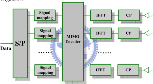
We consider the system which has M transmitting antennas and N receiving antennas. The transmitter architecture for MIMO-OFDM with space frequency block code system is shown in figure 3.1.

The data stream is mapped first, then these mapped signals are encoded by M/2 pairs of Alamouti code as shown in equation (3.1). For 4 transmitting antennas, 2 pairs of Alamouti code is called Double space time transmitting diversity (DSTTD) code as described in [12].

* 1 1 2 * 2 2 1 * 1 1 * 1 . . . . i . . M M M M M M S S S S S S S S S S S S − − − ⎡ − ⎤ ⎡ ⎤ ⎢ ⎥ ⎢ ⎥ ⎢ ⎥ ⎢ ⎥ ⎢ ⎥ ⎢ ⎥ =⎢ ⎥→ = ⎢ ⎥ ⎢ ⎥ ⎢ ⎥ ⎢ ⎥ ⎢ ⎥ ₋ ⎢ ⎥ ⎢ ⎥ ⎢ ⎥ ⎢ ⎥ ⎣ ⎦ ⎣ ⎦ S S (3.1)

Figure 3.1 Transmitter structure for MIMO-OFDM with space frequency block code

S/P

Signal mapping Signal mapping Signal mapping MIMO Encoder IFFT IFFT IFFT CP CP CP Data

The encoding process is shown as below : * * 1 2 ( _ / 2) 1 ( _ / 2) 2 * * 2 1 ( _ / 2) 2 ( _ / 2) 1 1 2 ( _ / 2) * * 1 ( _ / 2) 1 ( _ / 2) * * 1 ( _ / 2) ( _ / 2) 1 ... ... . . . , ,..., . . . ... ... M FFT len M M FFT len M M FFT len M M FFT len M M FFT len M M M FFT len M FFT len M M M FFT len M FFT len S S S S S S S S S S S S S S S S S S S − + − + − + − + − − − − − − → − − = (3.2) ⎡ ⎤ ⎢ ⎥ ⎢ ⎥ ⎢ ⎥ ⎢ ⎥ ⎢ ⎥ ⎢ ⎥ ⎢ ⎥ ⎢ ⎥ ⎣ ⎦ S

(where FFT_len is the length of a OFDM symbol),

The modulated signal S to ₁ S_{M fft len( _ / 2)} are encoded as equation (3.2). Each column vector

in matrix S represents an encoded signal vector allocated in a particular sub-carrier and each row vector in matrix S represents an encoded signal vector allocated in a particular antenna. As the graph shown below:

* *

1 2 ( _ / 2) 1 ( _ / 2) 2

*

2 1

Sub 1 Sub 2 ... Sub FFT_len ... 1 Tx antenna . 2 Tx antenna .. .. .. Tx antenna st M FFT len M M FFT len M nd th S S S S S S M − + − + − − → → → * ( _ / 2) 2 ( _ / 2) 1 * * 1 ( _ / 2) 1 ( _ / 2) * * 1 ( _ / 2) ( _ / 2) 1 .. . . . . . . ... ... M FFT len M M FFT len M M M M FFT len M FFT len M M M FFT len M FFT len S S S S S S S S S S − + − + − − − − ⎡ ⎤ ⎢ ⎥ ⎢ ⎥ ⎢ ⎥ ⎢ ⎥ ⎢ ⎥ ⎢ _{− −} ⎥ ⎢ ⎥ ⎢ ⎥ ⎣ ⎦

Then converts each row of matrix S by using Inverse Fast Fourier transform to time domain signal expressed in the next page.

* * 1 2 ( _ / 2) 1 ( _ / 2) 2 * * 2 1 ( _ / 2) 2 ( _ / 2) 1 * * 1 ( _ / 2) 1 ( _ / 2) * * 1 ( _ / 2) ( _ / 2) 1 ... ... . . . . . . ... ... M FFT len M M FFT len M M FFT len M M FFT len M M M M FFT len M FFT len M M M FFT len M FFT len S S S S S S S S S S S S S S S S − + − + − + − + − − − − ⎡ − − ⎤ ⎢ ⎥ ⎢ ⎥ ⎢ ⎥ ⎢ ⎥ ⎢ ⎥ ⎢ _{− −} ⎥ ⎢ ⎥ ⎢ ⎥ ⎣ ⎦ ⎯IFFT→ 1,1 1,2 1, _ 1 1, _ 2,1 2,2 2, _ 1 2, _ 1,1 1,2 1, _ 1 1, _ ,1 ,2 , _ 1 , _ ... ... . . . . . . ... ... FFT len FFT len FFT len FFT len M M M FFT len M FFT len M M M FFT len M FFT len s s s s s s s s s s s s s s s s − − − − − − − − ⎡ ⎤ ⎢ ⎥ ⎢ ⎥ ⎢ ⎥ ⎯⎯ ⎢ ⎥ ⎢ ⎥ ⎢ ⎥ ⎢ ⎥ ⎢ ⎥ ⎣ ⎦ (3.3)

Adding Guard interval for each row vector, then signals in each row are transmitted from different antenna. Since the encode process is implemented in frequency domain (subcarrier). We treat this type of code as space frequency block code.

3.2 MIMO-decoder

In receiver side, After guard interval removal and Fast Fourier transform, the received signals at n received antenna over subcarrier 1 and 2 are expressed as th

1, 1 2, 2 ( 1), 1 , * * * * * * 2, 1 1, 2 ( ), 1 ( 1), (1) (1) (1) ... (1) (1) (1) (2) (2) (2) .... (2) (2) (2) n n n M n M M n M n n n n M n M M n M n Y H S H S H S H S n Y H S H S H S H S n − − − − = + + + + + = − + + − + (3.4) ( ) n

Y k : Received signal of n th received antenna at k th sub-carrier

mn

H ( )k : Channel response in frequency domain for m th transmitting antenna and n th receiving antenna

m

S : m th mapped data

n

The matrix form representation for MIMO-OFDM 4X2 with space frequency block code system (for subcarrier 1 and 2) can be expressed as

Y = HS + N (3.5) 2 1 11 21 31 41 1 1 * * * * * * 1 21 11 41 31 2 1 2 12 22 32 42 3 2 * * * * * * 22 12 42 32 4 2 (1) (1) (1) (1) (1) (1) (2) (2) (2) (2) (2) (2) (1) (1) (1) (1) (1) (1) (2) (2) (2) (2) (2) (2) Y H H H H S n Y H H H H S n Y H H H H S n Y H H H H S n ⎡ ⎤ ⎡ ⎤ ⎡ ⎤ ⎢ ⎥ ⎢ _{− −} ⎥ ⎢ ⎥ ⎢ ⎥ ⎢₌ ⎥ ⎢ ⎥₊ ⎢ ⎥ ⎢ ⎥ ⎢ ⎥ ⎢ ⎥ ⎢ _{− −} ⎥ ⎢ ⎥ ⎢ ⎥ ⎣ ⎦⎣ ⎦ ⎣ ⎦ ⎡ ⎤ ⎢ ⎥ ⎢ ⎥ ⎢ ⎥ ⎢ ⎥ ⎣ ⎦ (3.6)

Where H is the equivalent channel matrix, S is the original symbol vector which is one of the columns in equation (3.2) and N is the additive complex white Gaussian noise with variance

2

σ .Assuming that H_mn(1)≈H_mn(2) and define

11 21 31 41 * * * * 21 11 41 31 12 22 32 42 * * * * 22 12 42 32 (1) (1) (1) (1) (1) (1) (1) (1) (1) (1) (1) (1) (1) (1) (1) (1) H H H H H H H H H H H H H H H H ⎡ ⎤ ⎢ _{− −} ⎥ ⎢ ⎥ = ⎢ ⎥ ⎢ _{− −} ⎥ ⎣ ⎦ eq H (3.7)

Multiplying H (where ()H_eq H represents Hermitian of a matrix) to the received vector we obtain

H H H

eq eq eq

Y = H Y = H HS + H N _(3.8),

Since we assumeH_mn(1)≈H_mn(2), for 4 transmitting antennas, the equivalent channel matrix

H will almost equal to H as shown _eq

11 21 31 41 11 21 31 41 * * * * * * * * 21 11 41 31 21 11 41 31 12 22 32 42 12 22 32 42 * * * * 22 12 42 32 (1) (1) (1) (1) (1) (1) (1) (1) (1) (1) (1) (1) (2) (2) (2) (2) (1) (1) (1) (1) (1) (1) (1) (1) (1) (1) (1) H H H H H H H H H H H H H H H H H H H H H H H H H H H H ⎡ ⎤ ⎢ _{− −} ⎥ _{− −} ⎢ ⎥ = ≈ ⎢ ⎥ ⎢ _{− −} ⎥ ⎣ ⎦ eq H * * * * 22 12 42 32 (3.9) (1) (2) (2) (2) (2) H H H H ⎡ ⎤ ⎢ ⎥ ⎢ _{⎥ =} ⎢ ⎥ ⎢ _{− −} ⎥ ⎣ ⎦ H So that 1 * * 1 2 * * 2 0 0 0 0 ρ α β ρ β α α β ρ β α ρ ⎡ ⎤ ⎢ ₋ ⎥ ⎢ ⎥ ≈ = ⎢ − ⎥ ⎢ ⎥ ⎣ ⎦ H H eq eq eq H H H H (3.10)