無刷直流馬達之分析與無感測器驅動之建模

全文

(1)國立交通大學電機與控制工程學系碩士論文. 無刷直流馬達之分析與無感測器驅動之建模. Analysis of BLDC Motors and Modeling of Sensorless Drive. 研究生：林翰宏指導教授：陳永平. 教授. 中華民國九十三年六月.

(2) 無刷直流馬達之分析與無感測器驅動之建模. Analysis of BLDC Motors and Modeling of Sensorless Drive 研究生：林翰宏指導教授：陳永平教授. Student：Han-Hung Lin Advisor：Professor Yon-Ping Chen. 國立交通大學電機與控制工程學系碩士論文. A Thesis Submitted to Department of Electrical and Control Engineering College of Electrical Engineering and Computer Science National Chiao Tung University In Partial Fulfillment of the Requirements For the degree of Master In Electrical and Control Engineering June 2004 Hsinchu, Taiwan, Republic of China. 中華民國九十三年六月.

(3) 無刷直流馬達之分析與無感測器驅動之建模. 學生：林翰宏. 指導教授：陳永平教授. 國立交通大學電機與控制工程學系. 摘要無刷直流馬達因其具高效率以及高功率密度，故至今在許多工業的應用領域中已受到較多的重視。然而為了迎接機器人時代的來臨，無刷直流馬達的應用必須更有效率、更有成效。為了達到這個目的，無刷直流馬達的特性將在論文中利用解析法及有限元素法作分析，並完整地建立一個以順滑觀測器為基礎的無感測器驅動方法。利用有限元素分析所得的結果可以建立一個詳盡的數學模型，以降低在實際系統上無法預測的錯誤。而所採用的無感測器驅動方法可以克服傳統無感測器驅動的啟動問題，使靜止啟動之馬達達到所需的轉速。在本論文中將完整呈現建立無感測器驅動系統的過程。. i.

(4) Analysis of BLDC Motors and Modeling of Sensorless Drive. Student：Han-Hung Lin. Advisor：Professor Yon-Ping Chen. Department of Electrical and Control Engineering National Chiao Tung University. ABSTRACT Up to now, BLDC motors are more attractive for many industrial applications due to high efficiency and high power density. However, for the coming of robotic generation, the utilization of BLDC motors should be more efficient and have better performance. In order to achieve this purpose, the characteristics of BLDC motors are analyzed by analytic and FEM based methods. Besides, an integrated sensorless drive method based on sliding mode observer is proposed. The results of FEM analysis are employed to establish an explicit mathematic model so that the unexpected error of the actual control system can be reduced. The proposed sensorless drive method is able to drive a BLDC motor from standstill to desired speed in wide speed range. The fault of start-up, which exits in conventional sensorless drive method, has been overcome. The integrated procedure for establishing the sensorless drive system of BLDC motors is presented in this thesis.. ii.

(5) Acknowledgment 本論文能順利完成，首先感謝指導老師陳永平教授這段期間來孜孜不倦的指導，讓作者在研究方法及語文能力上有著長足的進步，在為學處事的態度上亦有相當的成長，謹向老師致上最高的謝意；此外，感謝建峰學長於自身繁忙的博士研究之餘，仍抽空解答我研究上的疑惑以及給予建議，並不時給予我鼓勵，在此表達誠摯地感謝之意。最後，感謝口試委員鄭璧瑩老師以及張浚林老師提供寶貴意見，使得本論文能臻於完整。此外，還要感謝可變結構控制實驗室的克聰學長、豊裕學長、豐洲學長、培瑄、依娜、智淵、世宏、倉鴻以及學弟們對作者的照顧與陪伴，讓作者在實驗室的研究生活充滿溫馨與快樂。另外，感謝室友平修，在研究疲累的給予打氣，互相砥礪。最後，感謝父母與家人給予生活上的照顧與精神上的支持。謹以此篇論文獻給所有關心我、照顧我的人。林翰宏 2004.6.27. iii.

(6) Contents Chinese Abstract. i. English Abstract. ii. Acknowledgment. iii. Contents. iv. Index of Figures. vi. Index of Tables. ix. Chapter 1 Introduction .........................................................................................1 Chapter 2 Analysis of BLDC Motors ...............................................................3 2.1 Basic Concepts of Motors................................................................................3 2.2 Characteristics of BLDC Motors .....................................................................8 2.2.1 Magnetic Circuit Model........................................................................8 2.2.2 Flux Linkage and Back-EMF Voltage ................................................10 2.2.3 Self Inductance and Mutual Inductance..............................................12 2.3 FEM-Based Analysis .....................................................................................13 2.3.1 An Example to FEM Analysis of BLDC Motors ................................14. Chapter 3 Sensorless Drive of BLDC Motors .............................................17 3.1 Basic Operational Principle of BLDC Motors...............................................17 3.2 Concept of Sensorless Drives ........................................................................21 3.2.1 Back-EMF based Method ...................................................................21 3.2.2 Third-Harmonics Voltage....................................................................25 3.2.3 Observer-based Method ......................................................................26. iv.

(7) Chapter 4 Sensorless Drive Modeling ...........................................................30 4.1 Position Detection and Start-up Algorithm....................................................30 4.1.1 Initial Rotor Position Detection ..........................................................30 4.1.2 Start-up Algorithm ..............................................................................35 4.2 Sliding Mode Observer Design and the Estimations of Position and Velocity .....................................................................................................................38 4.2.1 Sliding Mode Observer Design for Position Estimation.....................38 4.2.2 Adaptive Velocity Estimation .............................................................44. Chapter 5 Simulation Result and Analysis ..................................................47 5.1 System Descriptions and Block Diagram ......................................................47 5.2 Simulation Result and Analysis .....................................................................51. Chapter 6 Conclusions and Future Works ..................................................59 Reference ..................................................................................................................61. v.

(8) List of Figures Fig. 2. 1 Electromechanical conversion system..........................................................3 Fig. 2. 2. Example of an electromechanical system.....................................................4. Fig. 2. 3. λ- i characteristic for the system in Fig. 2.2 for a particular air gap.............5. Fig. 2. 4. λ- i characteristic for energy and coenergy...................................................5. Fig. 2. 5. λ- i characteristic for constant current ..........................................................6. Fig. 2. 6. λ- i characteristic for constant flux linkage ..................................................6. Fig. 2. 7. Basic configuration of a rotating electromagnetic system............................7. Fig. 2. 8. Basic configuration of a PM motor ..............................................................8. Fig. 2. 9. The magnetic system included PM and winding........................................10. Fig. 2.10. The movement of the rotor ........................................................................ 11. Fig. 2.11 The flux linkage.........................................................................................11 Fig. 2.12. The back-EMF........................................................................................... 11. Fig. 2.13. The procedure of the FEM analysis...........................................................14. Fig. 2.14 The geometry and mesh of the brushless PM motor .................................15 Fig. 2.15. The magnetic line of force of the brushless PM motor .............................15. Fig. 2.16. The flux distribution of the brushless PM motor.......................................15. Fig. 2.17. The flux linkage of the path surrounding air gap ......................................16. Fig. 2.18. The back-EMF of the brushless PM motor ...............................................16. Fig. 3.1. Schematic of the inverter and equivalent modeling for a BLDC motor......19. Fig. 3.2. Torque production in a Y-connected three-phase motor. .............................19. Fig. 3.3. The procedure of six-step drive ...................................................................20. Fig. 3.4. Detection of switching point P from the crossing of the neutral voltage and terminal voltage. ..........................................................................................23. vi.

(9) Fig. 3.5. The back-EMF integration technique ..........................................................24. Fig. 3.6. Third-Harmonics Voltage technique............................................................26. Fig. 4.1. The flux linkage with positive or negative current......................................32. Fig. 4.2. The responses of current with positive or negative direction......................32. Fig. 4.3. The variation of inductance due to the change of the current and the rotor position ........................................................................................................33. Fig. 4.4. The current responses of the well-known six segments ..............................34. Fig. 4.5. The differences between the current in+ and in− ........................................34. Fig. 4.6. The differences between the current ∆in ...................................................35. Fig. 4.7. The torque generation of the six segments ..................................................37. Fig. 4.8. The current response of current the exciting and increasing segment.........37. Fig. 4.9. The block diagram of error equation ...........................................................44. Fig. 4.10. The block diagram of the adaptive velocity estimation.............................46. Fig. 5.1. A PMAC motor drive system with speed feedback control ........................47. Fig. 5.2. ® A PMAC motor drive system in Simulink .................................................48. Fig. 5.3 Speed responses of the system shown in Fig. 5.2........................................48 Fig. 5.4 A PMAC motor sensorless drive system .....................................................49 Fig. 5.5. The position and velocity sensorless control system...................................50. Fig. 5.6 Information of the D-axis current in case (I)...............................................51 Fig. 5.7 Information of the Q-axis current in case (I)...............................................52 Fig. 5.8. Information of the D-axis flux linkage in case (I) .......................................52. Fig. 5.9. Information of the Q-axis flux linkage in case (I) .......................................53. Fig. 5.10 Information of the rotor position in case (I) ..............................................53 Fig. 5.11. Information of the rotor velocity in case (I) ..............................................54. Fig. 5.12 Information of the rotor position in case (II).............................................54 vii.

(10) Fig. 5.13. Information of the rotor speed in case (II).................................................55. Fig. 5.14. Information of the rotor position with resistance variation .......................56. Fig. 5.15. Information of the rotor speed with resistance variation...........................57. Fig. 5.16. Information of the rotor position with inductance variation......................57. Fig. 5.17. Information of the rotor speed with inductance variation .........................58. viii.

(11) List of Figures Table 2.1 The electrical system and the magnetic system ........................................10 Table 4.1 Six segments of an electrical cycle ...........................................................34 Table 4.2 Polarity of ∆∆i k on rotor position ..........................................................35 Table 4.3 The exciting and increasing segment at electrical angle...........................37 Table 5.1 Specifications of motor .............................................................................48 Table 5.2 Parameters of observer and estimator .......................................................49. ix.

(12) Chapter 1 Introduction Motors are the conventional machines that transform the electrical power to the mechanical power. They play an important role in industry as well as in our daily lives. The development of motor technology grows up all the time so that a variety of motors are widely used in various applications. Comparing every kind of motors with their characteristics, the permanent magnet AC (PMAC) motors, which are also called brushless PM motors, are the most popular due to the reliability and efficiency. The PMAC motors offer many desired features, such as high efficiency, high torque to inertia ratio, high torque to volume ratio, high air gap flux density, high power to inertia ratio, high power to volume ratio, and compact structure. In detail, the PMAC motors are mainly divided into permanent magnet synchronous motors (PMSM) and brushless DC (BLDC) motors due to the induced back-EMF voltages. It is different from the PMSM with sinusoidal back-EMF that the BLDC motors have trapezoidal back-EMF. Each of them has specialized advantages and disadvantages. It is well known that the PMSM have high-performance and the BLDC motors have more power density and simpler commutation. In order to use the PMAC motors more efficiently, a variety of advanced control strategies are proposed, such as vector control and direct torque control. However, the rotor position sensors are needed to achieve electrical commutation in every strategy due to that the PMAC motors use permanent magnets for excitation. In general, Hall effect sensors or encoders are used as rotor position sensors for PMAC motors. Unfortunately, the rotor position sensors present several disadvantages in many applications when concerning the whole system’s cost, size, and reliability. 1.

(13) Therefore, recent investigators have paid more and more attentions to sensorless motors driving, which can be operated without any Hall sensors. Many sensorless-related technologies have been proposed, such as Back-EMF based position detection, third-harmonics voltage position detection, and Observer-based speed and position estimation. Up to now, sensorless motors driving is still a challenging and attractive topic For the robotics-generation applications, the utilization of motors should be more efficient and have better performance. In order to achieve this purpose, not only the better method of motor driving and controlling are required, but also the analysis of motor characteristics is needed. Therefore, in this thesis, the characteristics of BLDC motors will be discussed firstly. The analytic model and the Finite Element Method (FEM) based analysis will be presented in chapter 2. The principle of energy conversion in motor will be introduced and the output torque equation with respect to back-EMF will be derived. The simulation results of a BLDC motor based on FEM, including the path and the distribution of the magnetic flux, the flux linkage and back-EMF, will be shown. Then, an integrated sensorless drive method will be discussed in chapter 3 and chapter 4. The sensorless drive method proposed in this thesis can be employed to drive a PMAC motor from standstill in wide-speed application. The initial position of the rotor will be detected to avoid the temporary reverse rotation. After starting up successfully, a sliding observer is designed to estimate the rotor position and velocity by observing the flux linkage. It is noted that the estimations are robust to parameter variations. Finally, the simulation results of a sensorless drive system will be shown in chapter 5 by using Matlab®−Simulink®.. 2.

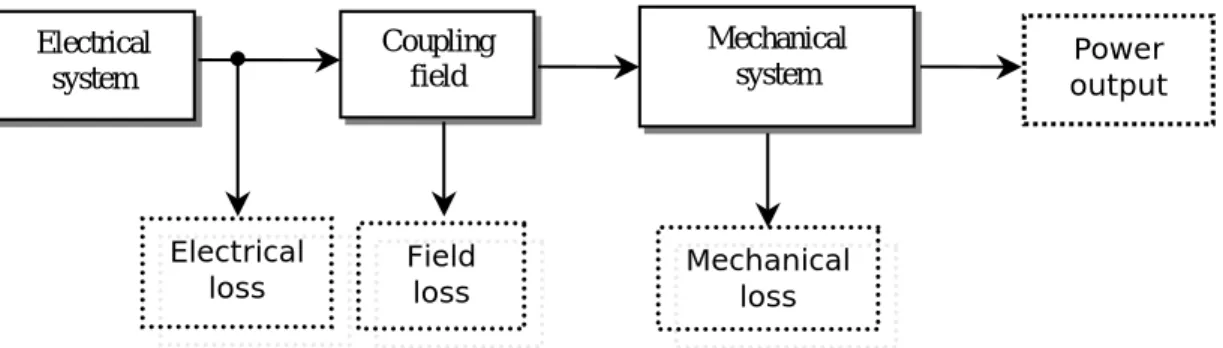
(14) Chapter 2 Analysis of BLDC Motors 2.1 Basic Concepts of Motors In general, motors convert electrical energy to mechanical energy by magnetic field to generate reaction torque. For the reaction torque, it is generated via the interactive force between windings with electric current and other magnetic fields, which is the so-called Lorentz force. It is required to know the electromechanical energy conversion in the motor before calculating its output torque, such as the reaction torque. There are various methods for calculating the output torque developed in energy conversion systems. It is difficult to calculate the power and the effect of each source in motor. The method usually used is based on the principle of conservation of energy, which states that energy can neither created nor destroyed. It can only be changed form one form to another. An electromechanical converter system has some essential parts as following.. Electrical system. Electrical loss. Coupling field. Mechanical system. Field loss. Mechanical loss. Power output. Fig. 2. 1 Electromechanical conversion system Consider Fig. 2.1, neglect the electrical loss, field loss and mechanical loss, the electromechanical converter system can be express as. dWe = dWm + dWf. (2-1) 3.

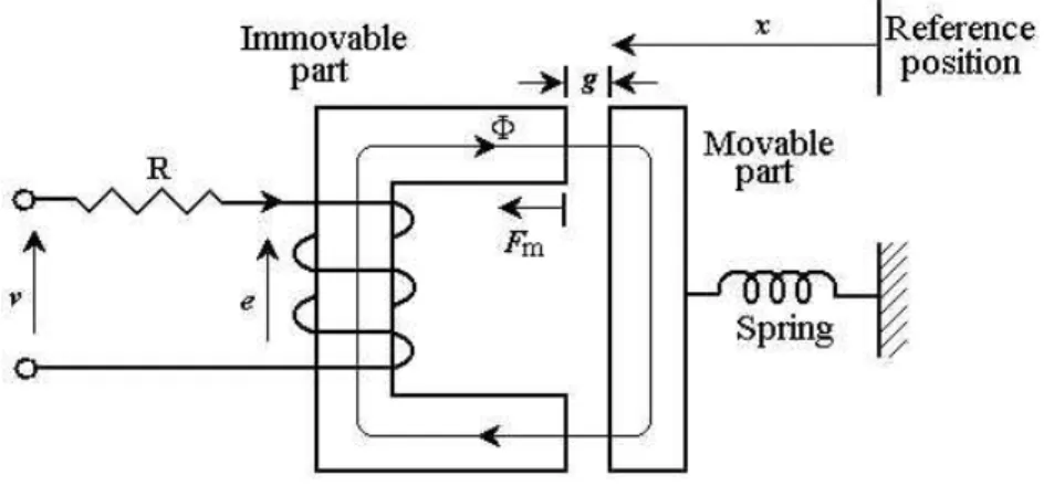
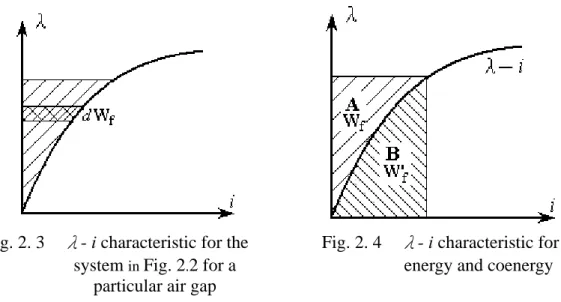
(15) where dWe is the increment of electrical energy flows to the system, dWf is the energy supplied to the magnetic field and dWm is the energy converted to mechanical form during time interval dt. Consider the electromechanical system of Fig. 2.2. If the system is stable, magnetic flux will be established in the magnetic system. Obviously, the mechanical energy can be expressed as. dWm = 0. (2-2). If core loss is neglected, form (2-1) and (2-2) and Faraday’s law, the energy of the magnetic field is derived as. dWf = i d λ. (2-3). The relationship between winding flux linkage λ and current i for a particular air gap length is shown in Fig. 2.3. When flux linkage form 0 to λ ′ , the field energy is expressed as. Wf = ∫. λ′. 0. idλ. (2-4). Furthermore, employing the concept of the coenergy, which is virtual field energy as shown in Fig. 2.4, the reaction torque can be obtained.. Fig. 2. 2. Example of an electromechanical system. 4.

(16) Fig. 2. 3. λ- i characteristic for the. Fig. 2. 4. system in Fig. 2.2 for a particular air gap. λ- i characteristic for energy and coenergy. According to Fig. 2.4, for a particular value of the air gap length, the area A represents the energy stored in field as derived above. The area B is so-called coenergy and is defined as i′. W ' f = ∫ λ di. (2-5). 0. Then, it is clear that. W ' f + Wf = λ i. (2-6). Consider the system shown in Fig. 2.2. If the moveable part move from a[x=x1] to. b[x=x2] then the air gap length decreases. Theλ− i characteristics of the system for these two position are shown in Fig. 2.5 and Fig. 2.6. If the movable part moved slowly, the current remained constant. The increment electrical energy, the magnetic field energy and the mechanical energy can be expressed as dWe = ∫. λ2. λ1. i d λ = area abcd. dWf = area 0 bc - 0 ad. (2-7) (2-8). dWm = dWe - dWf = area abcd + area 0 ad − area 0 bc = area 0 ab. (2-9). It is noted that the mechanical work represented by the shaded area in Fig. 2.5 is equal to the increment of coenergy. Thus, the mechanical force causing the differential. 5.

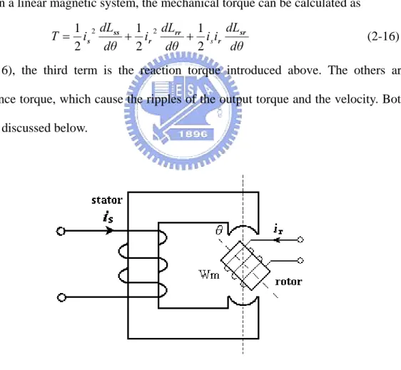
(17) displacement dx can be derived as f m dx = dWm = dW ' f ∂ W ' f (i, x) fm = ∂x. (2-10) i = constant. Employing the same principle, if the movable part moved quickly, the flux linkage remained constant, as shown in Fig. 2.6. The mechanical force causing the differential displacement dx can be derived as f m dx = dWm = − dWf fm = −. ∂ Wf (λ , x ) ∂x. (2-11) λ = constant. It is noted that in the limit when the differential displacement dx is small, the shaded area of Fig 2.5 and Fig 2.6 will be essentially the same. Therefore, the forces computed from (2-10) and (2-11) are equal.. Fig. 2. 5. λ- i characteristic for. Fig. 2. 6. constant current. λ- i characteristic for constant flux linkage. In order to realize the output torque in a motor briefly, consider a simple rotating machine system as shown in Fig. 2.7. The stored field energy dWf of the system can be evaluated as follow by establishing the currents is and ir.. dWf = i s d λ s + ir d λ r. (2-12). Assume that the magnetic system is linear, the flux linkage λ s of the stator winding and the flux linkage λ r of the rotor winding can be rewritten as 6.

(18) λ s = Lss i s + Lsr ir λ r = Lsr i s + Lrr ir. (2-13). where Lss is the self inductance of the stator winding, Lrr is the self inductance of the rotor winding and Lsr is the mutual inductance between stator and rotor windings. It should be noted that the values of these inductances are depend on the position of the rotor. Substituting (2-13) into (2-12), the filed energy dWf can be rewritten as. dWf = Lss i s di s + Lrr ir dir + Lsr d (i s ir ). (2-14). Integrating (2-14), the filed energy Wf can be obtained as. Wf =. 1 1 Lss i s2 + Lrr ir2 + Lsr i s ir 2 2. (2-15). Thus, in a linear magnetic system, the mechanical torque can be calculated as. T=. dL 1 2 dLss 1 2 dLrr 1 is + ir + i s ir sr dθ 2 dθ 2 2 dθ. (2-16). In (2-16), the third term is the reaction torque introduced above. The others are reluctance torque, which cause the ripples of the output torque and the velocity. Both will be discussed below.. Fig. 2. 7 Basic configuration of a rotating electromagnetic system. 7.

(19) 2.2 Characteristics of BLDC Motors The basic concepts of a rotating electromagnetic system have been introduced. The development of well-known induction motors is based on the concepts exactly. However, permanent magnet motors, whose rotor windings are replaced by permanent magnets, as shown in Fig. 2.8, are proposed for better performance and efficiency. PM motors are popular due to the high efficiency and the synchronization. The brushless DC motor is part of PM motors. In order to drive and control the BLDC motors more efficiently, the characteristics of BLDC motors will be discussed below.. Magnet N. Stator. S. Winding. Rotor. Fig. 2. 8 Basic configuration of a PM motor. 2.2.1 Magnetic Circuit Model. In BLDC system, (2-16) should be modified due to the permanent magnets. However, it is difficult to model the permanent magnets in the electrical circuit system. The concept of the equivalent magnetic circuit model should be employed. The corresponding relationship between electrical circuit system and equivalent magnetic circuit system is shown in Table 2.1. Considering the simple permanent magnetic 8.

(20) system as shown in Fig. 2.9 (a), the equivalent magnetic circuit can be obtained by using the theorems of Norton and Thevenin, as shown in Fig. 2.9 (b). Employing the principle of superposition, the total magnetic flux through the winding and magnet can be calculated as φ=. N1 I1 N2I2 + Rc + R g + R m Rc + R g + R m. φ r Rm N1 I1 = + Rc + R g + R m Rc + R g + R m. (2-17). where N1 , N 2. turns of winding and equivalent winding of magnet. I1 , I 2. current of winding and equivalent winding of magnet. Rc , R g , Rm. reluctance of core, air and magnet. φr. magnetic flux of magnet. It is well known that the flux linkage is the product of the turns and flux. From (2-5) and (2-17), the coenergy can be derived as follow by integrating with respect to current. 2. N N I I 1 N 22 I 22 1 N 12 I 1 + + 1 2 1 2 Wf′ = 2 R + Rm 2 R + Rm R + Rm =. NIR φ 1 N 12 I 12 1 (Rm φ r ) + 1 1 m r + 2 R + Rm 2 R + Rm R + Rm. =. 1 2 1 LI 1 + (R + Rm )φ 2m + N 1 I 1 φ m 2 2. 2. where R = R g + Rm L=. N 12 R + Rm. φm =. Rm φ r R + Rm. Then, (2-16) can be modified as 9. (2-18).

(21) T=. d φm ∂ Wf′ 1 2 dL 1 2 dR ′ = I1 − φm + N1 I1 dθ dθ 2 dθ 2 ∂θ. (2-19). Comparing (2-16) and (2-19), although the last two terms are changed due to the magnet, the first two terms are still reluctance torque and the third term is the reaction torque, which rotates the rotor mainly. Table 2.1 The electrical system and the magnetic system. Electrical system Source. electromotive force V. Flux. current. Impedance. resistance. Magnetic system magnetomotive force. F = Ni. i=. V R. magnetic flux. φ=. R=. ρl A. reluctance. ℜ=. (a). F ℜ l µA. (b). Fig. 2. 9 The magnetic system included PM and winding 2.2.2 Flux Linkage and Back-EMF Voltage. Considering a BLDC motor, ignoring the first two reluctance torque, the output electrical torque Te can be defined as Te = i s. d λf. (2-20). dθ. where is are stator phase currents and λf are the flux linkage between rotor PM and 10.

(22) stator phase winding. Assuming that the rotor is rotating at velocity ω , (2-20) can be expressed as ωTe = i s. d λf. (2-21). dt. According to the Faraday’s law, (2-20) can be rewritten as ωTe = i s e s. where es is defined as back-EMF voltage. In order to realize the torque generation in BLDC motors, consider the flux linkage and back-EMF. In BLDC motors, the flux linkage is coupling function of rotor PM and stator phase winding with respect to the rotor position. Assuming the rotor has the movement as shown in Fig 2.10, the flux linkage and the back-EMF are shown in Fig 2.11 and Fig 2.12. It is important to know about the relationship between the flux linkage/the back-EMF and rotor position due to that the maximum output torque is needed for driving efficiently.. (a). (b). ( c). Fig. 2.10 The movement of the rotor. π Position θe (rad). 2π. Fig. 2.11 The flux linkage. π Position θe (rad) Fig. 2.12 The back-EMF. 11. 2π.

(23) 2.2.3 Self Inductance and Mutual Inductance. The inductances are important to establish the mathematic model of a motor, which is needed for controlling. The inductances of a BLDC motor consist of the self inductance, and mutual inductance. Furthermore, the self inductance is divided into several parts, such as air gap inductance, slot leakage inductance and end turn leakage inductance. The analytic method for obtaining each is discussed explicitly in [BLDC design]. Each inductance can be calculated as. ns2 µ R µ 0 L τ c k d Lg = 4(l m + µ R k c g ). (2-22). ⎡µ d 2 L µ0 d2 L µ d L⎤ + 0 1 ⎥ Ls = ns2 ⎢ 0 3 + (ws + wsi ) / 2 ws ⎦ ⎣ 3 As. (2-23). n s2 µ 0 τ c ⎛ τ c π ⎞ ⎟ Le = ln ⎜⎜ ⎟ 8 4 A s ⎠ ⎝. (2-24). 2. Lm =. 1 Lg 3. (2-25). where Lg, Ls, Le and Lm are air gap inductance, slot leakage inductance, end turn leakage inductance, and mutual inductance. It is should be noted that above equations are derived at the assumption that the B-H curve of steel is linear.. 12.

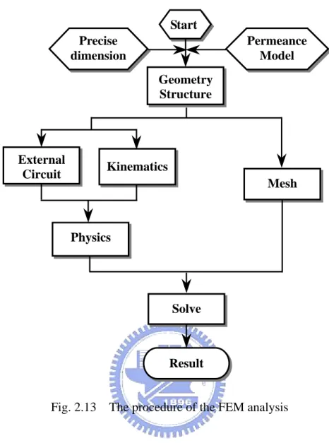
(24) 2.3 FEM-Based Analysis The advent of high speed microcomputers and available software has made possible the calculation of magnetic fields and torques of brushless DC motors. Finite Element Method (FEM) is an accurate tool of mathematical analysis. Recently, the approaches of using FEM to estimate the motor are quite common. FEM could have better performance in accuracy. Consequently, the following will adopt FEM to investigate the characteristic of brushless PM motors system. The software of Finite Element Approach, FLUX2D, will be adopted as the tool for simulation and analysis. This software was developed by MAGSOFT Company that possess twenty years experience in Professional Electromagnetism Analysis. Moreover, the software is known generally in internal academic world. The procedure of brushless PM motors analysis using Flux 2D will be introduced below, the flowchart is shown as Fig. 2.13. To start with the modification, it is necessary to establish the geometry structure of the motor. Then, defining the Physics and boundary condition, the model of the motor can be provided with power by the applied voltage, and analyzed by using Finite Element Method in the models of Transient Magnetic and Magnetodynamics. For the model of Transient Magnetic, the reluctance torque and the inductance variation can be obtained. For the model of Magnetodynamics, the kinematics of the rotor can be simulated after defining the rotational inertia, the coefficient of friction, the load, and driving algorithm. Furthermore, coupling the simulation result of the program, the approximately actual control system can be simulated. The unexpectable error of the actual control system can be reduced greatly.. 13.

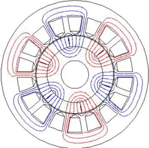
(25) Start Precise dimension. Permeance Model Geometry Structure. External Circuit. Kinematics Mesh. Physics. Solve. Result. Fig. 2.13 The procedure of the FEM analysis. 2.3.1 An Example to FEM Analysis of BLDC Motors. The brushless PM motor with 6 poles and 18 slots will be simulated by using Flux 2D program. The first the geometric structure of the motor should be established as shown in Fig. 2.14(a). The mesh needed for FEM analysis is generated automatically when the magnitude of mesh points is defined, as shown in Fig .2.14(b). After defining the physical characteristics and the boundary condition, the path and the distribution of the magnetic flux can be obtain, as shown in Fig. 2.15 and Fig. 2.16. Furthermore, the flux linkage and back-EMF can also be figured out while the external circuit and the driving algorithm are established.. 14.

(26) (a). (b). Fig. 2.14 The geometry and mesh of the brushless DC motor. Fig. 2.15 The magnetic line of force of the brushless DC motor. Fig. 2.16 The flux distribution of the brushless DC motor 15.

(27) Fig. 2.17 The flux linkage of the brushless DC motor. Fig. 2.18 The back-EMF of the brushless DC motor. 16.

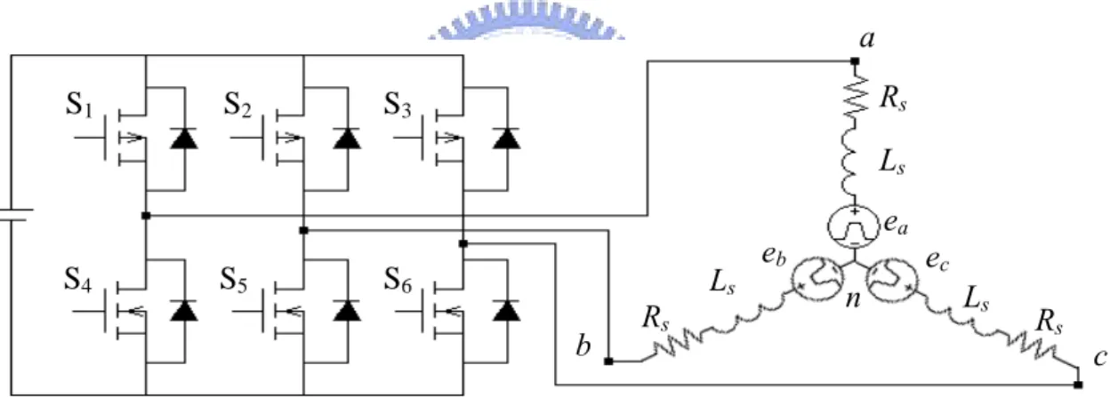
(28) Chapter 3 Sensorless Drive of BLDC Motors 3.1 Basic Operational Principle of BLDC Motors The BLDC motor has a rotor with surface-mounted magnets and stator windings, which are wound for the trapezoidal back electromotive forces. The trapezoidal back-EMF implies that the mutual inductance between the stator and rotor is non-sinusoidal. Therefore, when consider the mathematic model, it is no particular advantage to transform the phase variable equations of the BLDC motor into the well-known two-axis transformation (d, q model), which is done in the case of the permanent-magnet synchronous motors with sinusoidal back-EMF. The model of the three phases Y-connected BLDC motor consists of winding resistances, winding inductances, and back-EMF voltage sources. The inverter circuit and the equivalent model are shown in Fig. 3.1. Assume that rotor inducted currents can be neglected, no damper windings are modeled, the winding resistances are identical and the self and the mutual inductances are constant, which is independent of the rotor position. The voltage equations of the BLDC motor in phase variables can be given as ⎡v a ⎤ ⎡ R s ⎢v ⎥ = ⎢ 0 ⎢ b⎥ ⎢ ⎢⎣ vc ⎥⎦ ⎢⎣ 0. 0 Rs 0. 0 ⎤ ⎡ia ⎤ ⎡ L 0 ⎥⎥ ⎢⎢ib ⎥⎥ + ⎢⎢ M Rs ⎥⎦ ⎢⎣ic ⎥⎦ ⎢⎣ M. M L M. M ⎤ ⎡ia ⎤ ⎡ea ⎤ d M ⎥⎥ ⎢⎢ib ⎥⎥ + ⎢⎢eb ⎥⎥ dt L ⎥⎦ ⎢⎣ic ⎥⎦ ⎢⎣ ec ⎥⎦. where va, vb and vc. terminal voltages. Rs. winding resistance. ia, ib and ic. stator phase currents. 17. (3-1).

(29) L and M. self and mutual winding inductances. ea, eb and ec. phase back-EMF. Since ia + ic + ic = 0 , thus ⎡v a ⎤ ⎡ R s ⎢v ⎥ = ⎢ 0 ⎢ b⎥ ⎢ ⎢⎣ vc ⎥⎦ ⎢⎣ 0. 0 Rs 0. 0 ⎤ ⎡ia ⎤ ⎡ Ls 0 ⎥⎥ ⎢⎢ib ⎥⎥ + ⎢⎢ 0 Rs ⎥⎦ ⎢⎣ic ⎥⎦ ⎢⎣ 0. 0 Ls 0. 0 ⎤ ⎡ia ⎤ ⎡ea ⎤ d 0 ⎥⎥ ⎢⎢ib ⎥⎥ + ⎢⎢eb ⎥⎥ dt Ls ⎥⎦ ⎢⎣ic ⎥⎦ ⎢⎣ ec ⎥⎦. (3-2). with Ls = L − M. In state-space form the equations can be derived as ⎡i&a ⎤ ⎡1 / Ls 0 0 ⎤ ⎡ ⎡v a ⎤ ⎡ R s ⎢ ⎢& ⎥ ⎢ 1 / Ls 0 ⎥⎥ ⎢ ⎢⎢vb ⎥⎥ − ⎢⎢ 0 ⎢ib ⎥ = ⎢ 0 ⎢⎣i&c ⎥⎦ ⎢⎣ 0 0 1 / Ls ⎥⎦ ⎢⎣ ⎢⎣ vc ⎥⎦ ⎢⎣ 0. 0 Rs 0. 0 ⎤ ⎡ia ⎤ ⎡ea ⎤ ⎤ ⎥ 0 ⎥⎥ ⎢⎢ib ⎥⎥ − ⎢⎢eb ⎥⎥ ⎥ Rs ⎥⎦ ⎢⎣ic ⎥⎦ ⎢⎣ ec ⎥⎦ ⎥⎦ (3-3). and the electromagnetic torque and equation of motion are Te =. (ea ia + eb ib + ec ic ). (3-4). w. dw (Te − TL − Bw) = dt J. (3-5). where w. rotor speed. TL. external load. J. inertia. According to (3-4), the electromagnetic torque Te is dependent on the back-EMF and stator phase currents. The stator phase currents ia, ib and ic must be rectangular-shaped to produce a steady torque without pulsations due to the trapezoidal back-EMF. Besides, the currents ia, ib and ic should flow in only two of the three phases at any instant, and there should be no torque produced near the back-EMF zero crossing. The relationship between back-EMF and stator phase currents with respect to the electrical 18.

(30) degree θ e is shown in Fig. 3.2, where the electronic commutation statuses are also listed below the constant torque. With the electronic commutation statuses, the corresponding phase winding is excited to maintain the synchronization with the trapezoidal back-EMF such that the constant electromagnetic torque would be resulted. At each conduction period, one phase switch remains ON state with 120 electrical degrees and the other phase switches change states between ON, OF and short like as three-phase full bridge commutation. This drive method has lower copper utilization and more ohmic motor losses but lower cost than three-phase-ON drive. Since there are six commutations per electrical period, the drive scheme is so-called six-step drive. The detail commutation and excited procedure is illustrated with a two poles and six slots BLDC motor as shown in Fig. 3.3. a S1. S2. Rs. S3. Ls. S4. S5. S6 b. Rs. Ls. ea. eb. ec. n. Ls. Rs. Fig. 3.1 Schematic of the inverter and equivalent modeling for a BLDC motor.. Fig. 3.2 Torque production in a Y-connected three-phase motor. 19. c.

(31) b'. a. c. a. b. c. c'. a' b'. a. b c. a b. c. c'. a' b' b. a. c. a b. c. c'. a' b'. a. b c. a b. c. c'. a' b'. a. b c. a b. c. c'. a' b'. a. b c. a b. c. c'. a' b. Fig. 3.3 The procedure of six-step drive. 20.

(32) 3.2 Concept of Sensorless Drives Inherently, the BLDC motor is controlled electronically and requires rotor position information for properly commutating currents. In general, rotor position information is often measured by Hall sensors, which have been found to possess several disadvantages in many applications when concerning the whole system’s cost, size, and reliability. Therefore, recent investigators have paid more and more attentions to sensorless BLDC motors, which can be operated without any Hall sensors. Up to now, it is still a challenging and attractive topic. Many sensorless-related technologies have been proposed and the main methods can be primarily categorized as following: third-harmonics voltage-based position estimators [10], Back-EMF based position estimators [17], stator phase Observer-based speed and position estimators [3]. 3.2.1 Back-EMF based Method. In BLDC motor, the magnitude of a back-EMF induced in the stator windings due to the magnets is position dependent. Therefore, the rotor position can be accurately estimated in real-time and can be used to control the switching pattern of the inverter circuit by accurately monitoring the back-EMF, which is the commonest method for the sensorless drive system design due to its simple concept and implementation. The main back-EMF based method will be discussed below. In the basic BLDC motor operation, only two phases are excited at any instant and a back-EMF voltage can be measured from the terminals of the third phase conveniently. The zero-crossing method is employed to determine the switching sequence by detecting the instant where the back-EMF in the unexcited phase crosses zero. In general, when considering the inverter circuit is connected to a BLDC motor with Y-connected stator windings, as shown in Fig. 3.1, three terminal voltages va, vb 21.

(33) and vc can be derived as v a = v an + v n = Rs ia + Ls. dia + ea + v n dt. (3-6). vb = vbn + v n = Rs ib + Ls. dib + eb + v n dt. (3-7). vc = vcn + v n = Rs ic + Ls. dic + ec + v n dt. (3-8). where vn is the neural voltage, van, vbn and vcn are the phase voltages with respect to the negative DC bus, ia, ib and ic represent the phase currents, and ea, eb and ec are the back-EMF voltages generated in the three phases. In order to describe the zero-crossing method, for example S1 and S5 are ON, the terminal voltages va, vb and vc become v a = Vdc. (3-9). vb = 0. (3-10). v c = ec + v n. (3-11). Ideally, it is assumed that the current applied to the winding is rectangular-shaped and the stator inductance voltage drop is negligible. The relationship of the line-to-line current iab and corresponding phase currents ia and ib can be shown as iab = ia = −ib =. Vdc − (ea − eb ) 2 Rs. (3-12). According to (3-9), (3-10), (3-11) and (3-12), the terminal voltage of phase c can be derived as v c = ec + v n = ec +. Vdc − ea − eb 2. (3-13). Since the difference of 120° electrical degree in back-EMF voltage exists between any two phases, there is an instant that ec = 0 and ea = -eb. Then vc = v n =. Vdc 2. (3-14). Hence, the zero-crossing position of ec is independent of the load current. The terminal voltages va and vb have the same relationship as vc and vn at zero-crossing of 22.

(34) the back-EMF voltage when phase a or b is unexcited. After detecting the zero-crossing point of the unexcited phase, it is well know that the input signal to the unexcited phase should be given with 90° electrical degree delay to get the maximum torque, as shown in Fig. 3.4. The method can be realized by using voltage sensors and low-pass filters. However, the modulation noise is eliminated by using the low-pass filters, this causes a phase delay varies with the frequency of the excited signal for the desired rotor speed. Besides, the back-EMF voltage is zero at standstill and is proportional to the rotor speed. This method cannot be used at startup situation and works poorly at low-speed operation.. Fig. 3.4 Detection of switching point P from the crossing of the neutral voltage and terminal voltage.. The back-EMF integration technique can be also used for detecting the rotor position of BLDC motor. The phase-to-neutral voltage of unexcited stator winding is selected to measure the desired back-EMF, which is required for position sensing as soon as the residual inductive current flowing in the unexcited winding, immediately following the removal of excitation, decays to zero. The absolute value of this back-EMF is integrated as soon as the back-EMF crosses zero. Assume the back-EMF voltages are ideal trapezoidal waveforms, that is the unexcited phase back-EMF es. 23.

(35) varies linearly as e s (t ) = E 0 t. (3-15). where E0 is the slope of the unexcited phase back-EMF. Thus, the integrated voltage value vint can be obtained as e s (τ ) E t2 dτ = 0 0 k 2k. vint = ∫. t. (3-16). where k is the gain of the integrator. The next commutation signal is produced when the integrated voltage value vint reaches a pre-set threshold value as show in Fig. 3.5. The values of the threshold voltage and integrator gain depend on the motor and also on the alignment of the phase-current excitation waveform with the back-EMF. This method has the advantage of reducing the switch noise. Furthermore, since the back-EMF amplitude is proportional to the speed, the conduction intervals automatically scale inversely with the speed. Thus, there is an automatic adjustment of the inverter switching instants to changes in the speed. There are still other back-EMF based position estimation methods such as the phase-locked loop method and the free-wheeling diodes conduction method. However, all of them have the same disadvantage, not suitable for a wide-speed application due to that the low signal-to-noise ratio at low-speed operation causes the accuracy problem. ea eb ec vth vint Reset AC. 0o. BA. CB. 60 o. 120 o. AC 180 o. BA. CB 240 o. 300 o. Fig. 3.5 The back-EMF integration technique 24. 360 o. θe.

(36) 3.2.2 Third-Harmonics Voltage. As mentioned before, only two of the stator phases are excited at any instant. The stator currents flow into one of the excited windings and out of the other with 120 electrical degree square waves at each conduction periods. For maintaining the synchronization between the stator excitation and the MMF produced by the magnet, the six-inverter switches are switched at every 60 electrical degree. The switching can be detected by monitoring the third-harmonic voltage component of the back-EMF, which is a function of the rotor magnets and the stator winding configurations. For a full pitch magnet and full pitch stator phase winding, the back-EMF voltages contains the following frequency components ea = E (cosωe t + k 3 cos 3 ωe t + k 5 cos 5 ωe t + k7 cos 7 ωe t + ...). (3-17). eb = E (cos(ωe t − 2π / 3) + k 3 cos 3(ωe t − 2π / 3) + ...). (3-18). ec = E (cos(ωe t + 2π / 3) + k 3 cos 3(ωe t + 2π / 3) + ...). (3-19). Since the Y-connected stator windings, the third-harmonic voltages of the back-EMF produce no third-harmonic currents. The summation of the three stator phase voltages is a zero sequence which contains a dominant third-harmonic component and high frequency components, expressed as v an + vbn + vcn = 3 Ek 3 cos 3 ωe t + v high_freq = v 3 + v high_freq. (3-20). where v3 is the third-harmonic voltage and vhigh_freq is the high frequency components. Then, the third-harmonic rotor flux λr 3 can be obtained by integrating the third-harmonic voltage v3 as. λr 3 = ∫ v 3 dt. (3-21). It should be noted that the zero-crossings of the third-harmonic rotor flux occur at every 60 electrical degrees, which are exactly the switching instants mentioned above. Thus, the third-harmonic rotor flux is input to a zero-crossing detector and the output 25.

(37) of the zero-crossing detector determines the switching sequence, as shown in Fig. 3.6. The advantages of this method are simplicity of implementation, low susceptibility to electrical noise and robustness. This method has better performance in low-speed applications when comparing to the back-EMF based method. However, the sensing of the third-harmonic signal as described above requires access to the neutral connection of the stator phases or adopts an external resistance network to replace the neutral connection. Both of them have some undesirable influence. In most applications, the neutral terminal is not available due to the cost and structure constraints. The external resistance network causes the power lost and may change the characteristics of the motor.. ea eb ec v3. λr3 AC 0. o. BC 60. o. CA. BA 120. o. 180. o. 240. o. θe. AB. CB 300. o. 360. o. Fig. 3.6 Third-Harmonics Voltage technique 3.2.3 Observer-based Method. The last method listed above determines rotor position and speed using observers. The rough estimations of the angular rotor position by measuring the phase voltages and currents can be refined utilizing observers. The inputs of the observers are the inputs and outputs of the actual system such as phase voltages and currents;. 26.

(38) the outputs of the observers are the immeasurable states of the actual system such as flux linkage or back-EMF voltage. The states produced by the observer are fed back into the system, as would be the actually measured variables as used in a closed loop system control with specific rules for the various types of observers. For example, consider the discrete-time state-space form of a single output system, x[k + 1] = Ax[k ] + Bu[k ]. (3-22). y[k ] = Cx[k ] + Du[k ]. (3-23). which must be completely observable. Then, determine a modal matrix P for the system. Using the modal matrix P, the system is transformed into an observable form. x[k ] = Px ′[k ] = Q −1 x ′[k ]. (3-24). x ′[k ] = P −1 x[k ] = Qx[k ]. (3-25). x ′[k + 1] = A′x ′[k ] + B ′u[k ]. (3-26). y[k ] = C ′ T x ′[k ] + D T u[k ]. (3-27). where A′ = QAQ −1. B ′ = QB C ′ T = C T Q −1 Next, the full-order is designed for immeasurable states. The eigenvalues of the observer are usually chosen to be slightly faster than the eigenvalues of actual system such that the state estimated error approaches zero as time approaches infinity. If the eigenvalues of the observer are large enough, the estimated values will converge to the actual values within a sufficiently short time. The observer takes the form ζ ′[k + 1] = F ′ζ ′[k ] + g ′y[k ] + H ′u[k ]. where. F ′ = A′ − g ′C ′ T H ′ = B ′ − g ′d T 27. (3-28).

(39) with the observer output equation. w[k ] = Pζ ′[k ] = Q −1 ζ ′[k ]. (3-29). which allow the transformations. ζ [k ] = Pζ ′[k ] = Q −1 ζ ′[k ]. (3-30). ζ ′[k ] = P −1 ζ [k ] = Qζ [k ]. (3-31). ζ [k + 1] = Fζ ′[k ] + gy[k ] + Hu[k ]. (3-32). and gives. where. g = Q −1 g ′ F = Q −1 F ′Q = Q −1 A′Q − Q −1 g ′C ′ T Q = A − gC T H = Q −1 H ′ = Q −1 B ′ − Q −1 g ′d T = B − gd T Thus, the full-order observer in x[k] is derived, meaning that the immeasurable states can be obtained form ζ [k ] , which converges to x[k]. However, the full-order observer consists of more-order equations, the pole assignment is not easy and the manual tuning is time consuming. The reduced-order observers are developed for substitution. The reduced-order observers depend on that some of the system outputs are linear transformations of the system states. In motor drive application, the state, current, is readily available for measurement such that only the states, back-EMF voltages or flux linkages, need to be estimated by the lower-order observer. Assume that the sample rate of the system is fast enough; the sliding mode observers are available. The sliding mode observers, offspring of sliding mode control, utilize the varying switching function in order to confine the state estimation errors to approach toward zero on a phase-plane, sliding surface. For details, consider the state-space system. X& = AX + Bu. (3-33). y = CX. (3-34) 28.

(40) In BLCD systems, usually considering the PMSM or the fundamental of the trapezoidal BLDC, the state-space X consists of the d-q transformed stator variables. The state observer takes the same form with the addition of a switching input.. Xˆ& = AXˆ + Bu − K ⋅ sgn( S ). (3-35). where the hat symbol denoted estimated values. K is the switching gain and ⎧. 1. S≥0. ⎪− 1 ⎩. S<0. ⎪ sgn( S ) = ⎨. S is the vector of sliding surface Defining S = Xˆ − X = e , where e is the state estimation errors, the error equations can be derived as e& = Ae − K sgn(e ). (3-36). Consider the approach and sliding condition, let K be a large positive value to make sure the following equation hold. e T e& < 0. (3-37). Then, the observer states converge to the actual system states and the rotor position and the speed are estimated. Comparing to other methods, the achievement of rotor position estimation in wide speed and the real time estimation of the rotor speed are the critical grace. But the sampling rate, computational burden and the parameter variations need be considered.. 29.

(41) Chapter 4 Sensorless Drive Modeling 4.1 Position Detection and Start-up Algorithm The sensorless methods, which substitute for the Hall sensors or encoders to obtain the position information, have been introduced in the previous chapter. Each of them has specific advantages and drawbacks, but a common fateful fault. All of them can not detect the rotor position or speed at standstill or near zero speed with insufficient information required for estimating, such that are unable start-up. In order to overcome this fault, an extra start-up procedure, so-called “align and go”, has been proposed. As implied by the name, the algorithm is divided into two steps. First, excites any two phases winding of the stator to align the rotor to the specific position, and then accelerates the rotor according to the given firing sequences with decreasing time intervals. It should be noted that the initial position is not detected and the starting form unknown rotor position may be accompanied by a temporary reverse rotation or may cause a starting failure. These eventualities are not tolerable in many applications. Thus, a complete start-up procedure, which includes the detection of the initial rotor position and avoids the temporary reverse rotation or starting failure, should be developed [5]. The most proper method is based on the effect of the magnet position on the flux saturation, which cause the variations of the inductance. The details will be discussed below. 4.1.1 Initial Rotor Position Detection. Motors convert electrical energy to mechanical energy by magnetic field to generate desired torque, which is generated via the interactive force between windings. 30.

(42) with electric current and magnet. The path of the magnetic flux produced by the permanent magnet and current is a loop crossing the airgap to the stator from the rotor. Ideally, the B-H curve of the steel is linear and the inductance is constant due to the reluctance of the flux path is constant. But in practically, the B-H curve of the steel is a non-linear curve with saturation. Thus, the estimation of the rotor position can be detected by using the inductance variation due to the magnets position and the stator current. The relationship between inductance and flux linkage is shown as. λ Phase = λ PM + Li. (4-1). where λ Phase is the summation of the flux from the permanent magnet, λ PM , and the flux from the current i. L is the inductance of the excited phase. Supply the current with positive or negative direction to the phase, as shown in Fig. 4.1. The variations of the inductance are derived as L+ =. λPhase − λPM ∆λ + = i+ i+. (4-2). L− =. λPhase − λPM ∆λ − = i− i−. (4-3). where L+ and ∆λ+ are the inductance and flux linkage variation corresponding to the positive current i + is provided; L− , ∆λ − and i − is opposite. It is obvious that L+ is smaller than L− due to ∆λ + is smaller than ∆λ − . Consider the response of a phase voltage and current to the variation of the inductance. The phase voltage equation is expressed as van = Ri + L. di + ea dt. (4-4). The back-EMF can be neglect when a motor is at standstill. Then, solve the differential equation; the phase current can be derived as i=. v an R. R − t ⎞ ⎛ ⎜1 − e L ⎟ ⎜ ⎟ ⎝ ⎠. (4-5). According to (4-5), the phase current has a different transient dependent on the 31.

(43) inductance variation, which is determined by the relative position of the magnet and the direction of the current. It should be noted that i + has a faster response than i − due to the time constant R/L+ is larger than R/L− , as shown in Fig. 4.2. Therefore, the position information can be obtained by monitoring the phase current i + and i − in an appropriate time interval.. λphase λPM. ∆λ + ∆λ −. i−. i+. i. Fig. 4.1 The flux linkage with positive or negative current i. van R. i+. ∆i | i− |. T t Fig. 4.2 The responses of current with positive or negative direction. As mention above, the inductance variation with respect to the electrical angle should be known for detecting the rotor position. This problem can be overcome by using the FEM software, Flux 2D, to drawn out the relationship between inductance 32.

(44) and electrical angle, as shown in Fig. 4.3. Then, employing the information of inductance and (4-5) to gain the current responses with respect to the electrical angle in a time interval of 20 µs , as shown in Fig. 4.4 and Table 4.1 [5]. In Fig. 4.4, the current responses of the well-known six segments are calculated with the determined inductance in an appropriate interval of electrical degrees. Observing Fig. 4.4, it should be noted that the polarity of the difference between the positive current and negative current, ∆in , changes every 180 electrical degrees. Furthermore, the inherent differences with 120 electrical degrees exist in any two phases such that the polarity of one of three changes every 60 electrical degrees, which can provide the position information, as shown in Fig. 4.5 [5]. However, the position information from ∆in is not proper to drive a motor. The polarity of the difference between. ∆in − ∆i m , ∆∆i k , can be effectively used to identify the rotor position due to it includes the information of the polarity of the difference between two back-EMF used in six-step drive. The polarity of one of three ∆∆i k changes every 60 electrical degrees with 30 electrical degrees shift compared with the variation of ∆in , as shown in Fig. 4.6 and Table 4.2 [5]. Thus, the initial rotor position can be detected by monitoring the polarity of ∆∆i k , after each of six segments has been supplied a voltage pulse with a 20 µs period.. Fig. 4.3 The variation of inductance due to the change of the current and the rotor position 33.

(45) Fig. 4.4 The current responses of the well-known six segments. Table 4.1 Six segments of an electrical cycle Segment. Symbol of current i 1+. AB BA CA AC BC CB. i 1− i 2+ i 2−. i 3+ i 3−. (i) (ii) (iii) (iv) (v) (vi). Fig. 4.5 The differences between the current in+ and in− 34.

(46) Fig. 4.6 The differences between the current ∆in. Table 4.2 Polarity of ∆∆i k on rotor position. Electrical position. ∆∆ i1. ∆∆i 2. ∆∆i3. 30ο ~ 90ο. +. +. −. 90ο ~ 150ο. +. −. +. 150ο ~ 210ο. +. −. +. 210ο ~ 270ο. −. −. +. 270ο ~ 330ο. −. +. −. 330ο ~ 30ο. −. +. −. 4.1.2 Start-up Algorithm. In previous section, the initial position has been identified when a motor is at standstill. The correct phases winding on the stator are excited and the maximum electromagnetic torque is produced, so that the motor starts to rotation. Necessarily, the next commutation position should be detected for next excitation when the rotor rotates with 60 electrical degrees. However, the method proposed in previous section 35.

(47) is not suitable while the rotor is rotating due to the time delay caused by the period of six voltage pulses and the negative direction torque produced by exciting incorrect segments. Thus, a different start-up algorithm needs been developed. The start-up algorithm is also based on the principle of the previous section. Consider the torques produced by the six segments with respect to the electrical angle, as shown in Fig. 4.7. Except the exciting segment, which produces the maximum torque, there are still two segments to produce the torque with same direction in every commutation period. The torque of one is increasing and the other is decreasing. It should be noted that the increasing one is the next excitation. In other words, the increasing segment should replace the original exciting segment to be the new exciting segment while the torque produced by the increasing segment is larger than the torque produced by the original exciting segment. As to how to determine the magnitude of the torques, the test voltage pulse with a short time will be supplied into the increasing segment. Then, the switching point can be determined by comparing the current of the increasing segment with the current of the exciting segment due to the current is proportional to the torque. For example, the segment AC is excited when the initial position is detected as 30~60 electrical degrees. It means that the exciting segment is AC and increasing segment is BC . Then, cut off the segment AC and excite the segment BC with a shot time Ts in this commutation period, as shown in Fig. 4.8. The next excitation can be determined while the current of BC is larger than the current of AC . It means that BC replaces AC to be the exciting segment. The composition of the exciting segment and increasing segment with respect to electrical angle is shown in Table 4.3. The start-up algorithm can speed up a motor from standstill to a low speed, but is not suitable for high-speed operation due to the test voltage pulse.. 36.

(48) Fig. 4.7 The torque generation of the six segments. ON. 2*Ts. Ts. 2*Ts. Ts. 2*Ts. 90 ~ 150. ο. 30ο ~ 90ο. Ts. ο. current at. current at. OF. Fig. 4.8 The current response of current the exciting and increasing segment. Table 4.3 The exciting and increasing segment at electrical angle Electrical position. Exciting. Increasing. 30ο ~ 90ο. AC. BC. 90ο ~ 150ο. BC. BA. 150ο ~ 210ο. BA. 210ο ~ 270ο. CA. CB. 270ο ~ 330ο. CB. AB. 330ο ~ 30ο. AB. AC. 37. CA.

(49) 4.2 Sliding Mode Observer Design and the Estimations of Position and Velocity After a motor is successfully speeded up from standstill successfully, the rough start-up procedure should be replaced for better performance. In previous chapter, several well-known methods have been introduced and interpreted the characteristic and suitable application. Comparing these methods, the method based on the observer seems to have less constraint and more expansibility. Thus, the following section will discuss a sliding mode observer applied in sensorless BLDC system, which is considering the PMSM or the fundamental of the trapezoidal BLDC motors [4].. 4.2.1 Sliding Mode Observer Design for Position Estimation. The main purpose of the sensorless methods is to replace Hall sensors or encoders, which provide the rotor information. In order to achieve the purpose, it should be considered that what is relative to the rotor position. According to chapter 2, the back-EMF voltages or the flux linkages are most proper. Considering the stability, the flux linkages are chosen to observe due to the back-EMF voltage is the differentiation of the flux linkage. The equivalent circuit equation in the stationary reference frame, D-Q coordinate, is expressed as d ⎞ d ⎛ v = ⎜ R s + Ls ⎟ i + λ dt ⎠ dt ⎝. (4-6). where. v = [v D i = [i D λ = [λ D. vQ ]T iQ ] T. λQ ]T = [ K E ⋅ cosθ e 38. K E ⋅ sinθ e ]T.

(50) θ e rotor position at electrical angle K E EMF constant. It should be noted that (4-6) has a nonlinear term λ , which includes triangular function. Assume that KE is time independent such that the differentiation of λ can be rewritten as d ⎡ dθ λ = ⎢− e K E sinθ e dt ⎣ dt. T. [. dθ e ⎤ K E cosθ e ⎥ = − ω re λQ dt ⎦. ω re λ D ]. T. (4-7). where ω re is the rotational speed at electrical angle. Then, let stator current i and the flux λ be the state variables; the input is the stator voltage v and the output is the stator current i. Assuming that ω re is a constant parameter, the linear state equations can be expressed as. ⎡ i& ⎤ ⎡ A11 ⎢ &⎥ = ⎢ ⎣ λ⎦ ⎣ 0. A12 ⎤ ⎡ i ⎤ ⎡ B1 ⎤ v−D + A22 ⎥⎦ ⎢⎣ λ ⎥⎦ ⎢⎣ 0 ⎥⎦. ⎡i ⎤ i = C⋅⎢ ⎥ ⎣ λ⎦. (4-8). where A11 = −(Rs /Ls )I. A12 = −(ω re /Ls )J. A22 = ω re J. B1 = (1 /Ls )I. C = [I. ⎡0 J =⎢ ⎣1. 0]. − 1⎤ 0 ⎥⎦. The observability of the system can be verified by checking (4-8). Then, the sliding mode observer can be constructed as. ⎡ î& ⎤ ⎡ A11 ⎢ &⎥ = ⎢ ˆ ⎣⎢ λ ⎦⎥ ⎣ 0. A12 ⎤ ⎡ î ⎤ ⎡ B1 ⎤ ⎡I⎤ ⎢ ˆ ⎥ + ⎢ ⎥ v + K ⎢ ⎥ sgn î − i ⎥ A22 ⎦ ⎣ λ ⎦ ⎣ 0 ⎦ ⎣G ⎦. ( ). where. 39. (4-9).

(51) ∧. estimation state variable. K. switching gain. ⎡ g − g2 ⎤ G=⎢ 1 ⎥ ⎣ g2 g1 ⎦. feedback gain. Subtracting (4-8) from (4-9), the error equation can be derived as. ⎡ e&1 ⎤ ⎡ A11 ⎢ e& ⎥ = ⎢ 0 ⎣ 2⎦ ⎣. ( ). A12 ⎤ ⎡ e1 ⎤ ⎡I ⎤ ˆ + K ⎢G ⎥ sgn i − i + D A22 ⎥⎦ ⎢⎣ e 2 ⎥⎦ ⎣ ⎦. (4-10). where e1 = î − i is the current estimation error and e2 = λˆ − λ is the flux linkage estimation error and D is disturbances. Considering the state equations that the outputs of the system only include the currents in D-Q coordinate, the sliding mode is only applied to the current estimation. The sliding surface is selected as. s = e1 = î − i. (4-11). Then, employing the principle of Lyapunov, the approaching and sliding condition should be satisfied, as follow s T s& < −σ s. as. s≠0. (4-12). where σ > 0 . For details, (4-11) is subdivided as. e1 D e&1 D = −. R s 2 ω re e1 D + e1D e 2 Q + K e1 D + e1D D1 D Ls Ls. (4-13). e1Q e&1Q = −. R s 2 ω re e1Q − e1Q e 2 D + K e1Q + e1Q D1Q Ls Ls. (4-14). Thus, the switching gain K can be derived as. ⎡⎛ ω K < − n⋅ min ⎢⎜⎜ re e 2 Q + D1 D ⎣⎢⎝ L s. ⎞ ⎛ ω re ⎟ ,⎜ ⎟ ⎜ L e 2 D + D1Q ⎠⎝ s. ⎞⎤ ⎟⎥ ⎟ ⎠ ⎦⎥. (4-15). It should be noted that the magnitude of K has no influence on the response of the system. Usually, choosing n = 2 is enough for the sliding mode exciting. Under the sliding mode, the current estimation error is confined into the sliding surface as 40.

(52) e1 = e&1 = s → 0. (4-16). Furthermore, according to the principle of the equivalent control, the switching input can be treated as the equivalent input. Form (4-10) and (4-16), the equivalent inputs can be expressed as. ueq = − A12 e 2 − D. (4-17). Substituting the equivalent inputs into the second row of (4-10), the error equation of the flux estimation can be derived as. e& 2 = A′e 2 + D ′. (4-18). where. A′ = A22 − GA12 D ′ = [− G. I ]D. Form (4-18) and neglecting the disturbance, if all the eigenvalues of A′ are in the left-half plane of a complex plane, the estimated flux linkage will converge to the actual value. Calculating the eigenvalues of A′ , the relationship between the eigenvalues and feedback gain is given as eig ( A′) = −α ± j β. (4-19). where. α = g2. ω re L. β = ω re + g1. ω re L. However, it should be considered that where to assign the poles and the influence of the disturbance. Considering the closed-loop system form (4-18), the flux linkage estimation error can be derived as. e 2 (s ) = (s I − A′) D ′(s ) −1. (4-20). 41.

(53) Form (4-20), if the denominator order of the disturbance Laplace transforms is lower than one-order, the flux linkage estimation error will converge to zero due to the final value theorem. Form (4-7), the flux linkage is only relative to the velocity such that the velocity estimation error may lead to the flux estimation error. Therefore, the flux linkage estimation must be robust against the velocity estimation error. According to (4-9), the disturbance caused by velocity estimation error is express as T. ⎡ 1 Dω = ⎢− J ⎣ L. ⎤ J ⎥ ⋅ ˆλ ⋅ ∆ωre ⎦. (4-21). Substituting (4-21) into (4-20), the closed-loop transfer function T(s) can be derived as T (s ) = (s I − A′) Fω. (4-22). 1 Fω = − GJ + J L. (4-23). −1. where. Considering the block diagram, as shown as Fig. 4.9. In order to reduce the effect of the disturbance, the norm of T(s) needs been suppressed [1]. The frequency of flux linkage estimation changes widely with velocity. Considering the worst case, the capability of disturbance suppression can be quantitatively evaluated by the H ∞ norm. The H ∞ norm of the transfer function is calculated as T. ∞. = sup σ max [T ( j ω )] ω. [. ]. = sup λ max T * ( j ω ) ⋅ T ( j ω ) ω. Fω. = sup. (ω - β ). 2. ω. =. Fω. α. 2. (4-24). 2. +α 2 at. ω= β. where. σ max [⋅]. maximum singular value 42.

(54) λ max [] ⋅. maximum eigenvalue. ( )*. complex conjugate transposition. induced norm. 2. According (4-23), the induced norm of Fω can be calculated and expressed by using αand β, as Fω. 2. =. 1. ω re. α2 +β2. (4-25). Substituting (4-25) into (4-24) and letting β be equal to zero, the maximum capability of disturbance suppression is given as follow. min T. =. ∞. 1. (4-26). ω re. Furthermore, considering the transient response, α is assigned with respect to velocity, as. α = ν ω re. (4-27). where v is a factor to maintain the disturbance suppression [1]. From above, the current and the flux linkage have been estimated. The rotor position information can be obtained by using following equation.. ⎛ λQ ⎞ ⎟⎟ λ ⎝ D⎠. θ e = tan−1 ⎜⎜. (4-28). Then, the rotor position has been estimated without the influence of the back-EMF constant variation and robust to the parameter variation and velocity estimation error. As to how to determine the velocity, the details will be discussed in the next section. The estimation of velocity obtained from next section will be set as a parameter in above observer model.. 43.

(55) ˆλ ⋅ ∆ω. T(s). 1 Fω = − GJ + J L. 1 S. + +. e2. A′ = A22 − GA12 Fig. 4.9. The block diagram of error equation. 4.2.2 Adaptive Velocity Estimation. There are two conventional methods to estimate the velocity. Using the differentiation of the rotor position is the most common method. However, the noise may be included due to the differential operation and the PWM or switching signal. The other method employs the fact that the velocity is proportional to the magnitude of the back-EMF voltage, which is the differentiation of the flux linkage. However, the accuracy of the estimation is sensitive to the back-EMF constant variation and the direction of the velocity is unknown. Thus, the adaptive velocity estimation employing the estimated flux linkage λˆ is developed, as shown in Fig. 4.10. According to the relationship between the flux linkage and the velocity, the reference model is expressed as ˆλ& = ω Jˆλ re. (4-29). The estimation model is defined as 44.

(56) ~& ~ λ = ωˆ re Jλ. (4-30). ~ where λ is the output of the estimation model and ωˆ re is the estimated velocity.. Considering the convergence of the estimation error, the estimation model is adopted with a, as. (. ~& ~ ~ λ = ωˆ re Jλ − G ′ λˆ − λ. ). (4-31). where G ′ = g1′ I + g ′2 J. feedback gain. Taking the estimation error of the velocity into account, the estimation model with the closed-loop feedback is rewritten as. (. ~& ~ ~ ~ λ = ω re Jλ − (ω re − ωˆ re )Jλ − G ′ λˆ − λ. ). (4-32). From (4-29) and (4-32), the error equation can be derived as. & ~& ε& = λˆ − λ ~ = (ω re J + G ′)ε + (ω re − ωˆ re )Jλ. (4-33). = A′′ε + W and the adaptive scheme is chosen as ~. ωˆ& re = g ′ ε T Jλ. (4-34). where g ′ is the adaptive integral gain. Considering the convergence of the error equation, the poles of the closed-loop should be assigned in left-half plane as previous ~ section [2]. Then, the flux linkage estimation λ converges to the actual value and. the velocity estimation can be obtained by integrating (4-34). The velocity estimation consists of the direction and the magnitude and is robust to the variation of the back-EMF constant.. 45.

(57) Fig. 4.10. The block diagram of the adaptive velocity estimation. 46.

(58) Chapter 5 Simulation Result and Analysis In this chapter, the observer designed in chapter 4 is simulated by using Matlab®−Simulink®.. 5.1 System Descriptions and Block Diagram Generally, a PMAC motor drive system with speed feedback control consists of control algorithm, PWM generator and driver circuit, as shown as Fig. 5.1. According to (3-1), the motor model with the parameters shown in Table 5.1 is built as a block in Simulink®. Besides, the blocks of PWM driver and PI controller have also been built up. Connecting each block, a PMAC motor drive system, as Fig 5.1, is set up, as shown in Fig. 5.2. The simulation of speed control using PI controller is shown in Fig. 5.3. It is noted that the information of rotor position needed by driver is electrical angle, which is the product of mechanical angle and pole pairs.. Control algorithm. PWM generator. Driver circuit. Motor Load. Speed ref.. Speed feedback. Angle feedback. State vector. Fig. 5.1. A PMAC motor drive system with speed feedback control 47.

(59) Table 5.1 Specifications of motor Parameter. Symbol. Value. Unit. stator resistance. Ls. 8.5. [mH]. stator inductance. Rs. 2.875. [Ω]. inertia. Jm. 4e-3. [ kg ⋅ m2 ]. pole pairs. P. 3. EMF constant. KE. 0.175. Fig. 5.2. [Wb]. A PMAC motor drive system in Simulink®. command actual speed. Fig. 5.3 Speed responses of the system shown in Fig. 5.2 48.

(60) Then, replacing above system with sensorless drive system by using the sliding observer and adaptive estimator designed before, as shown in Fig. 5.4. The sliding observer and the adaptive estimator blocks are built up with the parameters shown in Table 5.2. The position and velocity sensorless control system is modeling in Simulink®, and the configuration of overall system as shown in Fig. 5.5. The sliding observer estimates the flux linkage from the phase voltages and currents. The rotor position can be obtained by using the estimated flux linkage. The velocity can be obtained by using the adaptive velocity estimation from the estimated flux linkage.. Motor Controller. PWM Generator. Motor Plant. Driver Circuit. voltage current. position velocity. flux linkage. Adaptive Estimator. Sliding Observer. Fig. 5.4 A PMAC motor sensorless drive system. Table 5.2 Parameters of observer and estimator Parameter. Symbol. Value. switching gain. K. -10000. feedback gain. g1. -8.5e-3. feedback gain. g2. 0.5*8.5e-3. feedback gain. g1′. ω re. feedback gain. g 2′. ω re. adaptive gain. KI. Unit. 15000000 [rad/s/Wb/A] 49.

(61) 50. Fig. 5.5. The position and velocity sensorless control system.

(62) 5.2 Simulation Result and Analysis In this section, several cases of different speed command are simulated. It is should be noted that the position and velocity sensorless estimation is switch on after the motor is started up successfully. Then, the information of feedback position and velocity is replaced with the estimation values while the motor is speeded up to 50 rpm. The method of start-up has been discussed in section 4.1, but it is not simulated here. Following simulations focus on the responses of the system at different speed commands and the robustness of the system to parameter deviations. First, the acceleration and deceleration from 60 rpm to 2000 rpm with rectangular speed command will be simulated with 50µs step size. Second, the acceleration and deceleration sinusoidal speed command will be simulated.. Fig. 5.6. Information of the D-axis current in case (I) 51.

(63) Fig. 5.7. Fig. 5.8. Information of the Q-axis current in case (I). Information of the D-axis flux linkage in case (I) 52.

(64) Fig. 5.9. Information of the Q-axis flux linkage in case (I). Fig. 5.10 Information of the rotor position in case (I) 53.

(65) Fig. 5.11 Information of the rotor velocity in case (I). Fig. 5.12. Information of the rotor position in case (II) 54.

(66) Fig. 5.13 Information of the rotor speed in case (II). According to the simulation results as shown above, there are several conclusions can be made. Without any parameter variation, the current estimation fits the actual current rapidly with a near zero error. It should be noted that the magnitude of the estimation error is related to the sampling rate. It is clear that the error is smaller when the sample rate is faster. From Fig. 5.8 and Fig. 5.9, the estimation of the flux linkage is robust to the velocity variation so that the position estimation has high accuracy with only 1 degree error, as shown in Fig. 5.10. The simulation result of the acceleration and deceleration from 30 rpm to 2000 rpm is shown in Fig. 5.11. The feasibility of the proposed method is verified at low and high speed. The desirable performance is also obtained in the second case. Then, the parameter variations will. 55.

(67) be considered in simulation. The 10% resistance variation and the 10% inductance variation will be put into the model. From Fig. 5.14 and Fig. 5.15, the steady flux linkage estimation and velocity estimation are not effected by the resistance variation, but the transient responses have bigger error. Comparing with the resistance variation, the inductance variation causes worse influence. The error of position estimation increases to 3 degree when the velocity is accelerated or decelerated, as shown in Fig. 5.16. In Fig. 5.17, a large error occurs in the velocity estimation at the instant of speed command changing. Summarily, the parameter variations cause the estimation error increasing. However, the magnitude of the error increment can still be tolerant due to the robustness.. Fig. 5.14. Information of the rotor position with resistance variation. 56.

(68) Fig. 5.15. Information of the rotor speed with resistance variation. Fig. 5.16. Information of the rotor position with inductance variation 57.

(69) Fig. 5.17. Information of the rotor speed with inductance variation. 58.