外國直接投資對印度尼西亞經濟增長的影響研究

(1)

INTERNATIONAL MASTER OF BUSINESS ADMINISTRATION

NATIONAL UNIVERSITY OF KAOHSIUNG

Master Thesis

AN IMPACT STUDY OF FOREIGN DIRECT

INVESTMENT ON ECONOMIC GROWTH IN

INDONESIA

Graduate Student：Andy Wijaya

Advisor：Prof. Po-Chih Lee

Prof. Chian-Hsueng Chao

(2)

(3)

An Impact Study of Foreign Direct Investment on

Economic Growth in Indonesia

Advisor(s): Prof. Po-Chih Lee

Prof. Chian-Hsueng Chao Department of International Business and Administration

National University of Kaohsiung Graduate Student: Andy Wijaya International Business and Administration

National University of Kaohsiung ABSTRACT

The purpose of this research is to test and analyze empirically the influence of foreign direct investment toward economic growth. The sample in this study is an annual report of Indonesia FDI and GDP in 1981 until 2017. This study also compared result of the previous research with this research. Data for this study comes from secondary data. The data was then analyzed with e-views 7 Panel Data Regression Analysis.

The results showed that simultaneous testing of significant effect of the independent variables measures foreign direct investment and trade openness with its dependent variable is economic growth. The result shows that both foreign direct investment and trade openness do have impact on Indonesia economic growth. These results are consistent with research by which is synonymous to the study results established by Younus et al. (2014), also consistent with the study by Ergin Akalpler and Hemn Adil1(2017) that there is a positive impact of foreign direct investment on economic growth. Busse and Ko¨niger (2012), and also study by Ergin Akalpler and Hemn Adil1(2017) also have some result that trade openness do have positive impact on economic growth

(4)

Table of Content

CHAPTER ONE INTRODUCTION

1.1 Background, motivation, and objectives……….. 1

1.2 Research Procedure……….. 7

CHAPTER TWO LITERATURE REVIEW 2.1 Economic Growth...………... 9

2.2 Foreign direct investment……… 10

2.3 How FDI impact Economic Growth……….. 12

2.4 Trade Opennes……… 13

2.4 Previous Study……… 14

2.5 Research Model……….. 16

CHAPTER THREE RESEARCH METHOD 3.1 Research Model………... 17

3.2 Population and Sampling………... 17

3.3 Definition Operational Variable and Variable Measurement…... 18

3.3.1 Dependent Variable………... 18

3.3.2 Independent Variable……….. 18

3.3.2.1 Foreign Direct Investment……….. 18

3.3.2.2 Trade Openness……….. 19

3.4 Data………..………... 19

3.5 Data analysis……… 19

3.5.1 VECM……. ……….. 20

(5)

3.5.2.1 Stationarity………... 20

3.5.2.2 Granger Casuality Test……… 21

3.5.2.3 Johansen Cointegration Test……… 22

3.6. Classic Assumption test………... 23

3.6.1 Serial Correlation Test...………... . 23

3.6.2 Heteroscedasticity Test...………... 23

CHAPTER FOUR DATA ANALYSIS AND REPORT 4.1 Sample ... 24

4.2 Time Series Analysis Choosing Method ... 24

4.2.1 Root Square Analysis………... 24

4.2.2 Lag Order Selection………. 25

4.3 Data Quality Test……….. ... 26

4.3.1 Stationarity Test………. 26

4.3.2 Johansen Cointegration Test……… 27

4.3.3 Granger Casuality Test……… 29

4.4 Vector Error Correction Model……... 30

4.5 Classic Assumption test……….... 31

4.5.1 Serial Correlation Test...………... . 31

4.5.2 Heteroscedasticity Test ...………... 32

CHAPTER FIVE CONCLUSION 5.1 Conclusion ... 33

5.2 Policy Suggestion ... 34

(6)

5.4 Recommendation for future study……… 35

REFERECE………... 36

(7)

TABLE CONTENT

Table 1.1 World Distribution of FDI ... 2

Table 1.2. GDP Growth in Indonesia ... 4

Table 4.1 Root Square test (eviews 7)... ... 22

Table 4.2 Lag order Selection Criteria (eviews 7) ... 23

Table 4.3 Augmented Dickey Fuller (eviews 7)... 24

Table 4.4 Philips Perron Test (eviews 7)... ... 25

Table 4.5 Johansen Cointegration Test (eviews 7)……… 26

Table 4.6 Granger causality–Block exogeneity test (eviews 7)……….27

Table 4.7 VECM result (eviews 7………... 28

Table 4.8 Breusch-Godfrey Serial correlation LM test. (eviews 7) ... 29

(8)

Figure Content

Figure 1. Proposed Dissertation Chapter... ... 7 Figure 2.1 Research Model... 14

(9)

1

Chapter 1. Introduction

1.1 Background , Motivation, and Objectives

Nowadays the measurement of how one country categorized as a success country is based on their economic growth, and the pioneer of this trend are China. China had enjoyed burst economic growth for the past decade, although the rate slowly decreasing down, but we can say that their government policies are success to generate more income and create more job opportunity inside their country. One major factor that lead China to become an overpower country is because how they open their domestic market to international investor, the easiness to open and invest in China generate FDI inflow to the country more than any developing country all over the world.

China success on increasing country’s economic growth using FDI inflow lead many scholars study the impact of FDI on another country. The study conduct to see the relationship between FDI and economic growth. Shiva s. Makki and Agapi Somwaru (2018) on their research find that FDI have been giving an improvement on country’s economic growth. They find that FDI are giving a positive stimulus toward domestic market, and the study result also explain that

(10)

2

country which had a great human capital likely give more advancement toward economic growth.

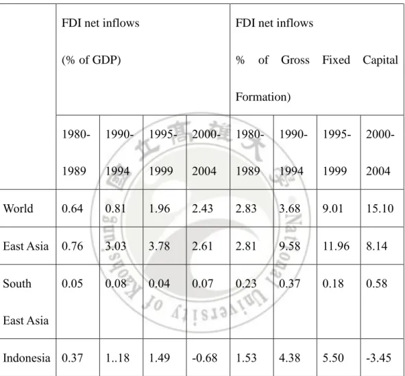
Table 1.1 World Distribution of FDI FDI net inflows

(% of GDP)

FDI net inflows

% of Gross Fixed Capital Formation) 1980-1989 1990-1994 1995-1999 2000-2004 1980-1989 1990-1994 1995-1999 2000-2004 World 0.64 0.81 1.96 2.43 2.83 3.68 9.01 15.10 East Asia 0.76 3.03 3.78 2.61 2.81 9.58 11.96 8.14 South East Asia 0.05 0.08 0.04 0.07 0.23 0.37 0.18 0.58 Indonesia 0.37 1..18 1.49 -0.68 1.53 4.38 5.50 -3.45

Data from the World Bank's World Development Indicators CD-ROM 2006. FDI net inflows: FX.KLT.DINV.CD.WD.

GDP: NY.GDP.MKTP.CD. And gross fixed capital formation: NE.GDI.FTOT.CD.

(11)

3

Many Country view FDI Inflow to host country as a source for transferring technology that later will generate the growth of host country economy. Many economic expertise based their research to find are FDI really affect the economic growth of host country or not.

The way to measure the implication of foreign direct investment to GDP can be seen by the volume of export and import, as said by Solow (1956) capital

input from other country outburst host country economic growth because transfer technology where there are going to be import new machine, and export new product from the new technology installed in host country.

So by putting new variable which was trade openness where means thw number of export and import on host country to determine the number of product sell outside the country that benefit on increase GDP also number of import where the technology assumed get transferred.

On the other situation Indonesia as one of the biggest country on south east Asia had enjoyed a positive economic growth for decade. But this growth is still far from enough to develop Indonesia from poverty and make Indonesia as one of developed country.

(12)

4

Indonesia’s president Joko Widodo the present leader of Indonesia is planning to attract more FDI to Indonesia, by opening more sector and relaxing the procedure to invest in Indonesia. This move, although seen as the maneuver for political issue but this moves are very realistic to generate Indonesia’s economy. By more relaxing the policies and procedural process, Indonesia trying to bring more investor to Indonesia. But in the past Indonesia had been open their market to overboard and generate lots of FDI inflow into Indonesia, as Abdul Khaliq and Ilan Noy (2007) mentioned the government of Indonesia started liberalizing its capital

account regime in 1967, when it introduced the Foreign Investment Law No. 1/1967. The government later adopted a free-floating foreign exchange system in 1970 which was followed by further liberalization of the financial sector in 1980s, the liberalization then lead Indonesia to 7,3% over the period 1970-1996, But the growth dropped when Asia face economic crisis.

(13)

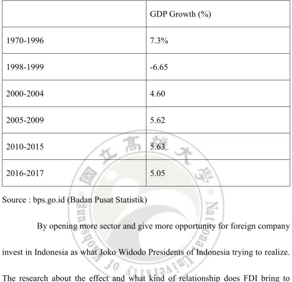
5 Table 1.2. GDP Growth in Indonesia

GDP Growth (%) 1970-1996 7.3% 1998-1999 -6.65 2000-2004 4.60 2005-2009 5.62 2010-2015 5.63 2016-2017 5.05

Source : bps.go.id (Badan Pusat Statistik)

By opening more sector and give more opportunity for foreign company invest in Indonesia as what Joko Widodo Presidents of Indonesia trying to realize. The research about the effect and what kind of relationship does FDI bring to Indonesia must be studied. Therefore can give some feedback and forecast on how FDI in fact effect Indonesia GDP and the result can give governor to formulate better policy in the future.

The research project will therefore seek to explore and investigate the following:  To examine the extent to which FDI and Trade Openness contribute to

(14)

6

 Offer policy recommendation for economic growth in Indonesia year 1981-2017.

(15)

7

1.2 Research Procedure

The research procedure are shown in figure 1.1. it civers steps as follows:

1. Introduction by giving explanation about research background, motivation, and objectives.

2. Reviewing Literature that consist of Independent Variables and Dependent Variables.

3. Data collection, data sampling, and analyze or research method are described in this section. Giving a concrete procedure how we study or analyze the data.

4. Utilizing Eviews to generate result and giving the implication and discussion.

5. Providing Conclusion, suggestions, limitations, and future research direction well.

(16)

8 Figure 1. Proposed Dissertation Chapter.

Chapter 1. Introduction

Chapter 2. Literature Review

Chapter 3. Methodology

Chapter 4. Result

Chapter 5. Conclusion

(17)

9

Chapter 2 Literature Review

Economic Growth

In general term Economic Growth define as an increase in economic value of good and service produced by an increase on nations ecomic scale.

As Solow (1956) mention on Makki and Somwaru (2004) long run growth can only arise because of technology progress and/or population growth, both considered exogenous. pioneering contribution to growth theory has generated the theoretical basis for growth accounting. In this neoclassical view, we can thus decompose the contribution to output growth of the growth rates of inputs such as technology, capital, labor, inward FDI, or by incorporating a vector of additional variables in the estimating equation, such as imports, exports, institutional dummies etc.

This is the building block of most growth analyses in economics. It follows the works of Solow (1956). The model assumes a neoclassical production function which postulates that the level of output and growth in an economy depends on the quantity of labor (L), capital (K) and knowledge and the effectiveness of labor (A). These inputs are combined to produce output through a function of the form Y(t) = F [K(t), A(t), L(t)], where „Y‟ is output and ‟t‟ represents time which enters the function indirectly through capital, labour and technology (Romer 2012).

(18)

10

The Solow Model forecasts that countries with low level of GDP per capita resulting from low capital accumulation in relation to long-run per capita are likely to experience growth rates and returns (Salai- i- Martin, 2004; Salai- i- Martin and Barro, 1995).

Foreign Direct Investment

FDI can be considered as a set of capital, technology, management, and entrepreneurship that enables an enterprise to work and deliver goods and services in a foreign market (Farrell, 2008).

According to Grazia Ietto-Gillies (2012) foreign direct investment and Multinational Corporation are the result of necoclassical economics principles. These theories were based on the classical theory of trade in which the motive behind trade was a result of the difference in the costs of production of goods between two countries, focusing on the low cost of production as a motive for a firm’s foreign activity.

Foreign Direct Investment (FDI) is an investment made abroad either by establishing a new production facility or by acquiring a minimum share of an already existing company (Bannoc~ Ethie, and Lawler at Accolley, 2006).

The World Bank defined FDI as investment that is made to acquire a lasting management interest in an enterprise operating in a country other than that of the investor (defmed according to residency). The investor's purpose is to gain an effective voice in the management of the enterprise.

(19)

11

Silajdzic and Mehic (2015) found that FDI is assumed to directly affect economic growth by contributing to the gross fixed capital formation.

The BPM5 (IMF Balance of Payments Manual, fifth edition) and the Benchmark (OECD Benchmark Definition of Foreign Direct Investment) in IMF (2001) define the concept of foreign direct investment as international investment by an entity resident in one economy in an enterprise resident in another economy that is made with the objective of obtaining a lasting interest. The lasting interest implies the existence of a long-term relationship between the direct investor and the enterprise and a significant degree of influence on the management of the enterprise. Direct investment involves both the initial transaction that establishes the relationship between the two entities and all subsequent capital transactions between them and among affiliated enterprises, both incorporated and unincorporated.

To the United Nations the countries that usually attract large amounts of FDI are those with good economic conditions, a certain high level of education, a high level of macroeconomic and political stability, favourable growth prospects and favourable investment environments. When the setting-up of a new site abroad is financed out of capital raised in the direct investor's country, FDI is referred to as greenfield investment (Lawler and Seddighi, 2001). The use of the term greenfield FDI has been extended to cover any investment made abroad by establishing new productive assets. It does not matter whether there has been a transfer of capital from the investor's country (home or source country) to the host country.

(20)

12

How FDI affect Economic Growth

In this literature we like to discuss how FDI effect economic growth and that is by considering FDI as a major contributor to the physical and financial capital of the host country, an increase in FDI is expected to lead to a high level of domestic capital stock needed for increased production. It can, therefore, be deduced from the neoclassical growth model that higher levels of capital stock coming from foreign economies through FDI results in higher growth of an economy. However, FDI in the neoclassical framework is seen as a contributor to growth only in the short run (Brems, 1970) since higher growth rate which is experienced after increasing the stock of FDI is only sustained in the short run.

On the other hand As Solow (1956) mention on Makki and Somwaru (2004), capital input from other country outburst host country economic growth because transfer technology where there are going to be import new machine, and export new product from the new technology installed in host country. So in this study Export and Import will be becoming control variable of study. The impact that come from either from export and import will be generalize as Trade openness. Ergin Akalpler and Hemn Adil1 (2017) also state that export and import have a important aspect to how FDI impact economic growth, by observe the trend on both of them we can know are the FDI input are about creating new market in host country or building new industry for old market abroad.

(21)

13

Trade Opennes

Trade openness is a measure of economic policies that either restrict or invite trade between countries. For example, if a country sets a policy of high trade tariffs, thus restricting the desirability of international trade, this restrictive policy will inhibit other countries from sending exports and accepting imports from that country.

Also according to Grazia Ietto-Gillies (2012) trade openness is the sum of imports and exports normalized by GDP. state that bilateral equity investment is strongly correlated with underlying patterns of trade. Investors are better able to attain accounting and regulatory information on foreign markets through trade and thereby invest in foreign assets.

Previous Study

The Impact of FDI to the economic growth had been a great study by some scholar, where they find out that on some cases FDI helping the economic growth of nation positively. Shiva S. Makki and Agapi Somwaru (2018) find out that FDI positively impact country economic growth, where they believe that happen because the technology transfer from developed country to the emerging developing country. On the other hand they also belive by lowering inflation rate, tax burden, and government consumption will help to increase the country economy performance.

Following the result Shiva S. Makki and Agapi Somwaru presented, Ergin Akalpler and Hemn Adil1 (2017) also stated the same result where the FDI

(22)

14

give the positive impact to economic growth in Singapore. The scholar remind the government although it appears it has a positive impact, but with bad policy handle by government will bring the opposite effect.

In contrast with what the other scholar presented, Mohamed Abdouli and Sami Hammami (2015) stated that not all the country has the same result where FDI impact the economic growth of one country. Their study find out that from all the MENA (Middle East-Non African) country 12 of them posed no significant effect into country economy growth. And also there is a negative relationship for Egypt and Lebanon.

Supporting the result of Mohamed Abdouli and Sami Hammami, Rami Hodrob (2017) also stated the same result where their study for Palestinian country lead him to find that there is negative relationship between FDI and economic growth. Which scholar believe happen because the lack of financial market, and the distribution of FDI did not focused on production sector.

Lim (200 I) surveys the recent literature of FDI's determinants and on the correlation between FDI and economic growth. From the survey, he concludes similar to de Mello, that there is relationship between FDI and economic growth.

Empirical investigations by Carkovic and Levine (2002) did not, also, enable to conclude about complementarities between FDI and human capital. Other recipient country's conditions are pointed to, in the literature, as a prerequisite for the growth effect of FDI via technology spill over. The result was ambiguous. Across countries, FDI appeared to have positive effects mainly in

(23)

15

financially developed countries. This evidence was not found applying panel estimators to the data. They investigated the hypotheses of complementarities between FDI and economic development, and FDI and trade openness. These hypotheses did not hold true.

Hermes and Lensink (2003) confirmed the finding using a panel data of 67 LDCs. The evidence they brought was not in favour of complementarities between FDI and human capital. They came up with evidence that the development of the domestic financial system is a necessary condition for FDI to generate positive externalities that increase output.

(24)

16

Figure 2.1 Research Model

Hypotheses

Based on previous study and the variable which used to determine Economic Growth then the hypotheses will be :

Ho1 : Foreign Direct Investment do impact Economic Growth

Ha1 : Foreign Direct Investment do not impact Economic Growth

Ho2 : Foreign Direct Investment do impact Trade openness

Ha2 : Foreign Direct Investment do not impact Trade Openness

Ho1 : Trade Openness do impact Economic Growth

Ha1 : Trade Openness do not impact Economic Growth

Economic Growth

Foreign Direct Investment

Trade Openness

(25)

17

CHAPTER III

RESEARCH METHOD

3.1 Research Model

The form of this research is a causal relationship, so here there are independent variables (variables that affect) and dependent variables (variables that are affected).

The dependent variable of this study is Gross Domestic Product. The independent variables of this study are foreign direct investment, trade openness

3.2 Population and Sampling Plan

The population of this research are foreign direct investment of Indonesia that listed on BPS (Indonesian Government’s Central Bureau Statistics). The observation period used was 37 years, namely 1981 to 2017. The sample in this study were foreign direct investment of Indonesia that listed on BPS (Indonesian Government’s Central Bureau Statistics) and Indonesian Coordinating Board for Investment (Badan Koordinasi Penanaman Modal, hereafter referred to as BKPM) on 1981 to 2017 selected using the nonprobability sampling method with purposive sampling technique, namely the selection of samples based on some criteria.

(26)

18

3.3 Definition Operational Variable and Variable Measurement

3.3.1 Dependent Variable

The dependent variable is the variable that is affected or which is due, because of the independent variables. The dependent variable in this study is gross domestic product. Busse and Ko¨niger (2012) define Gross domestic product is a monetary measure of the market value of all the final goods and services produced in a specific time period, often annually. This is defined as:

GDP

= Log(GDP)

3.3.2 Independent Variable

The independent variable is a variable that affects or is the cause of the change or the emergence of the dependent variable. The following independent variables are used in this study:

1. Foreign Direct Investmen

Foreign Direct Investment (FDI) measure the total level of direct investment at a given point in time, usually the end of a quarter or of a year.Foreign direct investments defined as:

(27)

19

2. Trade Openness

Busse and Ko¨niger (2012) explained trade as the amount of exports and imports as a lag of GDP. In their study, they determined that trade had a strong and significant impact on economic growth. Trade openness defined as

Trade Openness =

Log (Export+Import)

3.4 Data

Data is“the fact and figures collected, analyzed, and summarized for

presentation and interpretation” (Anderson et al. 2014, 5)

Data collection techniques used in this study are secondary data sources, namely sources that do not directly provide data to data collectors. The data used is the annual foreign direct investment report published by BKPM from 1981 to 2017, and also from balance sheet published by BPS (Indonesian Government’s Central Bureau Statistics). Data collection was obtained from the Indonesia Coordinating Board for Investment (bkpm.go.id) and Indonesian Government’s Central Bureau Statistics (bps.go.id).

3.5 Data Analysis

The statistical method used to test hypotheses is a method simple regression statistics (simple linear regression) and multiple regression analysis (multiple linear regression). While processing data using Eviews.

(28)

20

3.5.1 Vector Error Correction Model

Ergin Akalpler and Hemn Adil (2017) define that Vector Error Correction

Model as systematic method with the features that the variation of the

contemporary state from its long-run association will be incorporated into its short-run dynamics. And in the model there should be a cointergration between variables and if there is no contintegration then we should assume VAR as the best method.

VECM are best to conduct on research that use time series model. Therefor before we conduct the test we need to determine which method are best to use either VECM or VAR, and to answer that we must find if there a cointegration between variables or not.

3.5.2 Data Quality Test

3.5.2.1 Statinoary

Standard regression analysis methods, such as ordinary least squares (OLS), necessitate that the variables are covariance stationary. A variable is considered to be covariance stationary if the mean as well as the auto-covariances are finite and do not alter over time. Cointegration analysis presents a system for estimation, inference, and interpretation when the variables are not covariance stationary. Moreover, rather than being covariance stationary, the majority of economic time series can be observed to be ‘‘first-difference stationary’’. Accordingly, this implies that in such situations, the time series’ level is not stationary, however the first difference is. First difference stationary processes are

(29)

21

also referred to as integrated processes of order 1, or alternatively, I (1) processes. However, covariancestationary processes are I (0). We used the Augmented Dickey Fuller and the Phillips Perron tests to determine if the series is stationary or not.

3.5.2.2 Granger Casuality Test

The Granger causality test is an analytical foundation test that is used to estimate whether a one-time series can be beneficial for forecasting another. Under normal conditions, regressions merely demonstrate associations; however, Clive Granger asserted that, for the purposes of economics, the causality could be calculated by measuring the capacity to estimate the probable values of a time series by utilizing the values from a previous time series. As the topic of ‘‘true causality’’ is profoundly complex, and because of the post hoc ergo propter hoc logical fallacy that states that one event following another event can be used as evidence for causation, econometricians assert that Granger analysis only reveals ‘‘predictive causality’’.

A time series X is claimed to Granger-cause Y if it can be explained customarily by a group of F tests and t tests on lagged values of X (and with lagged values of Y also included), that those X values offer statistically vital knowledge about the xpected values of Y.

(30)

22

3.5.2.3 Johansen Cointegration Test

The Johansen co-integration test is a combination of the Maximum Eigenvalue test and the Trace test. The most distinguishing feature between the Maximum Eigenvalue test is that it subjects the null hypothesis of r co-integrating equations against the alternative of r ? 1 cointegrating equations.

In which, the sample size is denoted by T and the Maximum Eigenvalue by k. This expression implies that trace statistics are subject to testing the hypothesis of co-integrating equations (r), together with the alternative hypothesis of n cointegrating equations. Thus, the number of variables is denoted by n. The Trace statistic can be derived using the following expression:

LRMAX (𝒓

𝒏+ 𝟏) = -T*Log(1-)

In which, the sample size is denoted by T and the Maximum Eigenvalue by k. This expression implies that trace statistics are subject to testing the hypothesis of co-integrating equations (r), together with the alternative hypothesis of n cointegrating equations. Thus, the number of variables is denoted by n. The Trace statistic can be derived using the following expression:

LRTrace (𝒓

𝒏+ 𝟏) = -T*∑ 𝒍𝒐𝒈(𝟏 −) 𝒏

𝟏=𝒓+𝟏

It must be noted that computation of the Johansen Co-integration test may yield different results and, if such a case manifests, then the Trace statistic results are more preferable than the Maximum Eigenvalue statistics.

(31)

23

3.6. Classic Assumption Test

3.6.1 Heteroskedasticity test

Breusch–Pagan test, developed in 1979 by Trevor Breusch and Adrian Pagan, is used to test for heteroskedasticity in a linear regression model. The null hypothesis is that there is no heteroskedasticity, i.e. the variance of the dependent variable is homoskedastic. Heteroscedasticity tends to underestimate variance of the estimators, causing high F and t statistics values.

3.6.2 Serial Correlation Test

The serial correlation test was conducted using the Breusch-Godfrey Serial correlation LM test. The null hypothesis is that there is no autocorrelation. Autocorrelation occurs when the error terms are correlated. Alternatively, the presence of autocorrelation signifies that the error terms are independently distributed.

(32)

24

Chapter IV

ANALYSIS AND DISCUSSION

4.1 Sample

The sample that will be examined in this study are annual report of foreign direct investment and annual report of economic and gdp (growth domestic product) in the period of 1980-2017.

4.2 Time Series analysis choosing method

4.2.1 Root square analysis

Root square test used to determine the number of lag used for analysis. The criteria for choosing number of lag are akaike criteria information and

Schwarz criterion. The criteria for choosing must shown the lesser number.

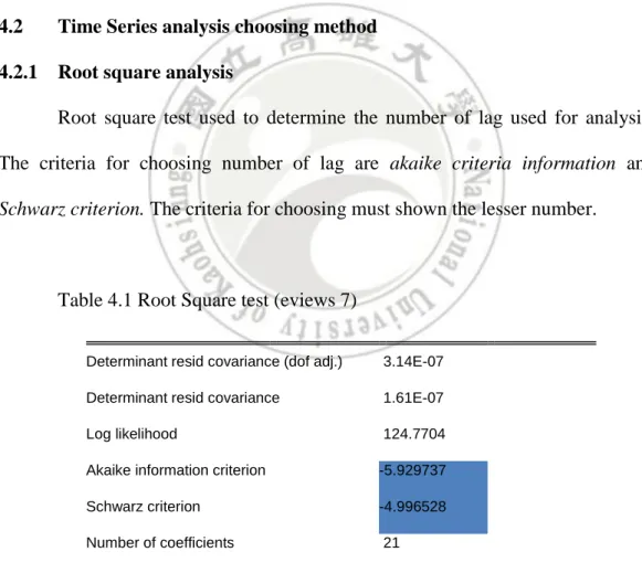
Table 4.1 Root Square test (eviews 7)

Determinant resid covariance (dof adj.) 3.14E-07 Determinant resid covariance 1.61E-07

Log likelihood 124.7704

Akaike information criterion -5.929737 Schwarz criterion -4.996528 Number of coefficients 21

(33)

25

From the result showt at table 4.1 akaike criteria information has -5.929737 and Schwarz criterion has -4.996528, so from the result we choose

akaike criteria information.

4.2.2 Lag order selection

Damodar N. Gujarati (2003) said that for annual report used on time series the maximum number of lag can be used either 1 or 2 as not to lose the number of freedom of analysis. The criteria for choosing are the number shown for must lower than the the other number.

Table 4.2 Lag order Selection Criteria (eviews 7)

VAR Lag Order Selection Criteria

Endogenous variables: GDP FDI TRADE_OPENNES Exogenous variables: C

Sample: 1981 2017 Included observations: 35

Lag LogL LR FPE AIC SC HQ

0 3.295949 NA 0.000197 -0.016911 0.116404 0.029109 1 112.5383 193.5150 6.44e-07 -5.745045 -5.211782* -5.560963 2 124.7704 19.57139* 5.43e-07* -5.929737* -4.996528 -5.607594*

(34)

26

The number shown at akaike criteria information column tell that the number lag that best to use for analysis is 2, lag1 = -5.745 and lag 2 = -5.929. so the number of lag used for analysis are 2.

4.3 Data Quality test

4.3.1 Statinoary Test

Stationarity of a series (that is, a variable) implies that its mean, variance and covariance are constant over time. That is, these do not vary systematically over time. In order words, they are time invariant. To know are the data are stationary or not we use Augmented Dickey Fuller and the Phillips Perron tests. H0 :  0.5 = Data are stationary

Ha :  0.5 = Data are not stationary

Table 4.3 Augmented Dickey Fuller (eviews 7)

NO Variable

At Level At first difference

none Constant Trend none Constant Trend

1 GDP 0.9998 0.4253 0.8963 0.0296 0.0074 0.0012 2 FDI 0.9216 0.1230 0.2418 0.00 0.00 0.00 3 Trade Opennes 0.9968 0.2329 0.8508 0.00 0.00 0.00

(35)

27

Table 4.4 Philips Perron Test (eviews 7)

From two table shown at table 4.3 and table 4.4 show that data are stationary at first difference as their number less than  = 0.5, so the research will be using first difference when finding the vector error correction model.

4.3.2 Johansen Cointegration Test

The main purpose behind the Johnsen Cointegration test is to determine if long equilibrium associations exist between the variables. Computed Eigenvalue and Trace Statistics can be used to determine the number of cointegrating equations. The Johansen Cointegration test proposes the null hypothesis that there are no cointegrating equations at 5% significance level. The decision criterion is to accept the null hypothesis of no cointegrating equations when the obtained probability is greater than 5%.

NO Variable

At first difference

none Constant Trend

1 GDP 0.0296 0.0076 0.0012

2 FDI 0.0000 0.0000 0.0000

(36)

28

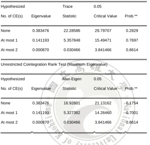
Table 4.5 Johansen Cointegration Test (eviews 7)

Unrestricted Cointegration Rank Test (Trace)

Hypothesized Trace 0.05

No. of CE(s) Eigenvalue Statistic Critical Value Prob.** None 0.383476 22.28586 29.79707 0.2829 At most 1 0.141193 5.357848 15.49471 0.7697 At most 2 0.000870 0.030466 3.841466 0.8614 Unrestricted Cointegration Rank Test (Maximum Eigenvalue)

Hypothesized Max-Eigen 0.05

No. of CE(s) Eigenvalue Statistic Critical Value Prob.** None 0.383476 16.92801 21.13162 0.1754 At most 1 0.141193 5.327382 14.26460 0.7001 At most 2 0.000870 0.030466 3.841466 0.8614

Using the Maximum Eigenvalue statistic and Trace method indicates the presence of cointegration. The Trace statistic results number shows are bigger in value and also because trace test are more favorable Thus, the Trace statistic results will be used to estimate a VECM of the impact of FDI on economic growth in Indonesia. The main emphasis is to determine if there is a long-run or short-run association between the dependent variable and the independent variables.

(37)

29

The result of the test show that there is a cointergration between variables so its mean that the method for analyzing are VECM.

4.3.3 Granger causality–Block exogeneity test

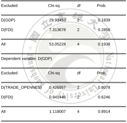
Table 4.6 Granger causality–Block exogeneity test (eviews 7)

Dependent variable: D(TRADE_OPENNES)

Excluded Chi-sq df Prob.

D(GDP) 29.93452 2 0.1839 D(FDI) 7.313678 2 0.2858

All 53.05228 4 0.1938

Dependent variable: D(GDP)

D(TRADE_OPENNES) 0.426957 2 0.8078 D(FDI) 0.941446 2 0.6246

All 1.118007 4 0.8914

Dependent variable: D(FDI)

D(TRADE_OPENNES) 0.073528 2 0.9639 D(GDP) 0.041484 2 0.9795

(38)

30

The Block exogeneity test is also conducted to establish if there is a causality between the variables in the long-run. The results are presented in Table 4.9. All of the obtained Chi Square probability results are greater than 5% and thus, the hypothesis that there is no causality between the variables in the long-run is accepted at 5%. Therefore, all the variables do not Granger cause each other in the long-run.

4.4 Vector error correction model results

The VECM was estimated using 2 lag and cointegrated at 1 equation. The results show that there is no long-run causality that runs from GDP, FDI, and TO. The results are presented in Table 4.7 The normalized cointegrating coefficients are shown below:

GDP = 0.029771 + 0.006630 FDI + 0.05561TRADE_OPENNES+E Table 4.7 VECM result (eviews 7)

Variables Coefficient Standard error T- F -statistics

FDI(-1) 0.006630 0.819384 2.176050

TRADE_OPENNES(-1) 0.055613 0.031150 9.160246

C 0.029771 - _-

ECt-1 0.041645 0.041645 0.522480

The results presented in Table 4.7 exhibit that there is a positive association between GDP and FDI of 0.00663. This means that a 1% increase in foreign direct investment results in a positive increase in GDP by 0.06%. This result reinforces the study results obtained by Ergin Akalpler and Hemn Adil1 (2017), which have shown strong evidence that A possible explanation could be the fact that employment levels rise as FDI is put into effective use. Moreover,

(39)

31

FDI inflows can have widespread gains when they are accompanied by new technology, which improves efficiency and effectiveness in production. Such improvements can lower costs of production and result in mass production and, hence, more resources can be expended on theproduction of other goods. This propels an upward increase in GDP

The results also exhibit that there is a positive linkage between GDP and trade opennes of 0.055613. This translates to an increase in GDP by 0.0556 units following an increase in trade opennes by 1 unit. A possible explanation could be the fact that there are transfer of technology and new market open at aboard as Export and Import that keep rising, and thus stimulate the economic growth.

4.5 Classic Assumption Test

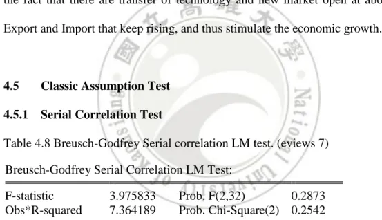
4.5.1 Serial Correlation Test

Table 4.8 Breusch-Godfrey Serial correlation LM test. (eviews 7) Breusch-Godfrey Serial Correlation LM Test:

F-statistic 3.975833 Prob. F(2,32) 0.2873 Obs*R-squared 7.364189 Prob. Chi-Square(2) 0.2542

The serial correlation test was conducted using the Breusch-Godfrey Serial correlation LM test. The null hypothesis is that there is no autocorrelation. Autocorrelation occurs when the error terms are correlated. Alternatively, the presence of autocorrelation signifies that the error terms are independently distributed. Using the results obtained and shown in Table 4.7, it can be observed

(40)

32

that the obtained Chi square value is 0.2542, which is more than 5% and thus we accept the null hypothesis of no autocorrelation.

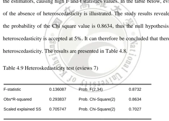
4.5.2 Heteroskedasticity test

Breusch–Pagan test, developed in 1979 by Trevor Breusch and Adrian Pagan, is used to test for heteroskedasticity in a linear regression model. The null hypothesis s that there is no heteroskedasticity, i.e. the variance of the dependent variable is homoskedastic. Heteroscedasticity tends to underestimate variance of the estimators, causing high F and t statistics values. In the table below, evidence of the absence of heteroscedasticity is illustrated. The study results revealed that the probability of the Chi square value is 0.8634, thus the null hypothesis of no heteroscedasticity is accepted at 5%. It can therefore be concluded that there is no heteroscedasticity. The results are presented in Table 4.8.

Table 4.9 Heteroskedasticity test (eviews 7)

F-statistic 0.136087 Prob. F(2,34) 0.8732 Obs*R-squared 0.293837 Prob. Chi-Square(2) 0.8634 Scaled explained SS 0.705747 Prob. Chi-Square(2) 0.7027

(41)

33

CHAPTER 5

CONCLUSION LIMITATIONS, AND RECOMMENDATION

5.1. Conclusion

This study aims to obtain empirical evidence of FDI and TRADE OPENNES on Indonesia economic growth (dependent variable) listed on the period 1981-2017. Based on the discussion and research described in the previous chapter, the following conclusions are obtained:

1. Foreign Direct Investment affects Economic Growth positively. These results are consistent with research by which is synonymous to the study results established by Younus et al. (2014), also consistent with the study by Ergin Akalpler and Hemn Adil1(2017)

2. Trade Opennes affects Economic Growth positively. These results are consistent with research by which is synonymous to the study results established by Busse and Ko¨niger (2012), also consistent with the study by Ergin Akalpler and Hemn Adil1(2017).

Thus the conclusion of this study that all the independent variables affect economic growth positively and sifnificantly, namely, foreign direct investment and trade opennes

(42)

34

5.2. Policy Suggestion

From the result of study, researcher can summarize a few point of recommendation for government economic policy considering FDI and trade openness. The suggestion cand described as:

1. Provide support for FDI by making a regulation to give easiness to open business or slim down the paperwork so the environment of business is more attractive.

2. Trade Openness do impact the economic growth and belived to generate the technology transfer to host country. So government should decrease the tariff imposed to product categorized as technology transfer and also decrease tariff export.

5.2. Limitations for future study

The author realizes that there are limitations to this study. Limitations in this study include:

1. This research only covers Indonesia as objet population, and also the time period that not long enough..

2. Limited variables, which only use independent variables, namely foreign direct investment and trade openness.

(43)

35

5.3. Recommendation for future study

Based on the limitations that have been submitted by researchers, the researchers suggest some recommendations that are expected to be useful for further researchers who want to raise a similar theme. Some of the authors' recommendations are as follows:

1. Using a broader research object so as to produce a greater number of samples.

2. Adding the number of other variables to the research that might explain and contribute to profitability.

(44)

36

Reference

Abu1 Nurudeen., Abd. Karim Moh. Zaini. (2016). The Relationships Between Foreign Directinvestment, Domestic Savings, Domestic Investment, And Economic Growth: The Case Of Sub-Saharan Africa. Society and

Economy 38 (2016) 2, pp. 193–217.

Adam Samuel., (2009). Foreign Direct investment, domestic investment, and economic growth in Sub-Saharan Africa. Journal of Policy Modeling 31 (2009) 939–949.

Anderson, David R., Dennis J. Sweeney., William Thomas A. 2008, 2014.

Statistics for Business and Economics. 12thEdition. South Western: Cengage Learnings.

Borensztein, E., De Gregorio, J., & Lee, J. (1998). How does foreign direct investment effect economic growth. Journal of International Economics, 45, 115–135.

Borhan, H., Ahmed, E. M., & Hitam, M. (2012). The impact of CO2 on economic growth in Asean 8. Procedia Social and Behavioral Sciences, 35, 389–397. Breusch, T. S., & Pagan, A. R. (1979). A simple test for heteroskedasticity and

random coefficientvariation. Econometrica, 47(5), 1287–1294.

Ergin Akalpler, Hemn Adil. (2017). The impact of foreign direct investment on economic growth in Singapore between 1980 and 2014. Eurasian Econ

Rev (2017) 7:435–450.

Khaliq Abdul, Noy Ilan. (2007). Foreign Direct Investment and Economic Growth: Empirical Evidence from Sectoral Data in Indonesia. New Economics

Papers (2007), 07-26.

Mohamed Abdouli1, Sami Hammami. (2017). The Impact Of FDI Inflows And Environmental Quality On Economic Growth: An Empirical Study For The MENA Countries. J Knowl Econ (2017) 8:254–278.

Shiva S. Makki And Agapi Somwaru (2018). Impact Of Foreign Direct Investment And Trade On Economic Growth: Evidence From Developing Countries.

Solow, R. M. (1956). A contribution to the theory of economic growth. Quarterly Journal of Economics 70, 65–94. (reprinted in Stiglitz and Uzawa 1969).

(45)

37

Younus, H. S., Sohail, A., & Azeem, M. (2014). Impact of foreign direct investment on economic growth in Pakistan. World Journal of Economics

(46)

38 CHOOSING LAG CRITERIA

Vector Autoregression Estimates Sample (adjusted): 1983 2017

Included observations: 35 after adjustments Standard errors in ( ) & t-statistics in [ ]

Determinant resid covariance (dof adj.) 3.14E-07 Determinant resid covariance 1.61E-07

(47)

39

VAR Lag Order Selection Criteria

Endogenous variables: GDP FDI TRADE_OPENNES Exogenous variables: C

Sample: 1981 2017 Included observations: 35

Lag LogL LR FPE AIC SC HQ

0 3.295949 NA 0.000197 -0.016911 0.116404 0.029109 1 112.5383 193.5150 6.44e-07 -5.745045 -5.211782* -5.560963 2 124.7704 19.57139* 5.43e-07* -5.929737* -4.996528 -5.607594*

(48)

40 STATIONARITY TEST

ADF AT LEVEL

Null Hypothesis: GDP has a unit root Exogenous: None

Lag Length: 1 (Automatic - based on AIC, maxlag=2)

t-Statistic Prob.* Augmented Dickey-Fuller test statistic 3.616304 0.9998 Test critical values: 1% level -2.632688

5% level -1.950687 10% level -1.611059

Null Hypothesis: GDP has a unit root Exogenous: Constant, Linear Trend

t-Statistic Prob.* Augmented Dickey-Fuller test statistic -2.295538 0.4253 Test critical values: 1% level -4.243644

5% level -3.544284 10% level -3.204699

Null Hypothesis: GDP has a unit root Exogenous: Constant

5% level -2.948404 10% level -2.612874

(49)

41 AT FIRST DIFFERENCE

Null Hypothesis: D(GDP) has a unit root Exogenous: None

5% level -1.950687 10% level -1.611059

Null Hypothesis: D(GDP) has a unit root Exogenous: Constant, Linear Trend

5% level -3.544284 10% level -3.204699

Null Hypothesis: D(GDP) has a unit root Exogenous: Constant

5% level -2.948404 10% level -2.612874

(50)

42 FDI

AT LEVEL

Null Hypothesis: FDI has a unit root Exogenous: None

5% level -1.951000 10% level -1.610907

Null Hypothesis: FDI has a unit root Exogenous: Constant, Linear Trend

5% level -3.540328 10% level -3.202445

Null Hypothesis: FDI has a unit root Exogenous: Constant

5% level -2.945842 10% level -2.611531 0.9216 0.1230 0.2418

(51)

Null Hypothesis: D(FDI) has a unit root Exogenous: None

5% level -1.951332 10% level -1.610747

Null Hypothesis: D(FDI) has a unit root Exogenous: Constant, Linear Trend

5% level -3.552973 10% level -3.209642 Null Hypothesis: D(FDI) has a unit root

Exogenous: Constant

5% level -2.954021 10% level -2.615817

(52)

44 OPEN TRADENESS

AT LEVEL

Null Hypothesis: TRADE_OPENNES has a unit root Exogenous: None

5% level -1.950394 10% level -1.611202

Null Hypothesis: TRADE_OPENNES has a unit root Exogenous: Constant, Linear Trend

5% level -3.540328 10% level -3.202445

Null Hypothesis: TRADE_OPENNES has a unit root Exogenous: Constant

5% level -2.945842 10% level -2.611531 0.9968 0.2329 0.8508

(53)

Null Hypothesis: D(TRADE_OPENNES) has a unit root Exogenous: None

5% level -1.950687 10% level -1.611059

Null Hypothesis: D(TRADE_OPENNES) has a unit root Exogenous: Constant, Linear Trend

5% level -3.544284 10% level -3.204699

Null Hypothesis: D(TRADE_OPENNES) has a unit root Exogenous: Constant

5% level -2.948404 10% level -2.612874

(54)

46 PP TEST

GDP

AT FIRST DIFFERENCE

Null Hypothesis: D(GDP) has a unit root Exogenous: None

Bandwidth: 0 (Newey-West automatic) using Bartlett kernel

Adj. t-Stat Prob.* Phillips-Perron test statistic -2.185609 0.0296 Test critical values: 1% level -2.632688

5% level -1.950687 10% level -1.611059

Null Hypothesis: D(GDP) has a unit root Exogenous: Constant, Linear Trend

5% level -3.544284 10% level -3.204699

Null Hypothesis: D(GDP) has a unit root Exogenous: Constant

5% level -2.948404 10% level -2.612874 0.0296 0.0076 0.0012

(55)

47 FDI

AT FIRST DIFFERENCE

Null Hypothesis: D(FDI) has a unit root Exogenous: None

5% level -1.950687 10% level -1.611059

Null Hypothesis: D(FDI) has a unit root Exogenous: Constant, Linear Trend

5% level -3.544284 10% level -3.204699

Null Hypothesis: D(FDI) has a unit root Exogenous: Constant

5% level -2.948404 10% level -2.612874

(56)

48 TRADE OPENNESS

AT FIRST DIFFERENCE

Null Hypothesis: D(TRADE_OPENNES) has a unit root Exogenous: None

5% level -1.950687 10% level -1.611059

Null Hypothesis: D(TRADE_OPENNES) has a unit root Exogenous: Constant, Linear Trend

5% level -3.544284 10% level -3.204699

Null Hypothesis: D(TRADE_OPENNES) has a unit root Exogenous: Constant

5% level -2.948404 10% level -2.612874

(57)

49 JOHANSEN COINTEGRATION TEST

Sample (adjusted): 1983 2017

Included observations: 35 after adjustments Trend assumption: Linear deterministic trend Series: GDP FDI TRADE_OPENNES Lags interval (in first differences): 1 to 1 Unrestricted Cointegration Rank Test (Trace)

Hypothesized Trace 0.05

No. of CE(s) Eigenvalue Statistic Critical Value Prob.** None 0.383476 22.28586 29.79707 0.2829 At most 1 0.141193 5.357848 15.49471 0.7697 At most 2 0.000870 0.030466 3.841466 0.8614 Unrestricted Cointegration Rank Test (Maximum Eigenvalue)

Hypothesized Max-Eigen 0.05

No. of CE(s) Eigenvalue Statistic Critical Value Prob.** None 0.383476 16.92801 21.13162 0.1754 At most 1 0.141193 5.327382 14.26460 0.7001 At most 2 0.000870 0.030466 3.841466 0.8614 Max-eigenvalue test indicates no cointegration at the 0.05 level

* denotes rejection of the hypothesis at the 0.05 level **MacKinnon-Haug-Michelis (1999) p-values

Unrestricted Cointegrating Coefficients (normalized by b'*S11*b=I):

(58)

50 VECM

Vector Error Correction Estimates Date: 12/26/19 Time: 06:04 Sample (adjusted): 1984 2017

Included observations: 34 after adjustments Standard errors in ( ) & t-statistics in [ ]

Cointegrating Eq: CointEq1 GDP(-1) 1.000000 FDI(-1) -0.352934 (0.13047) [-2.70518] TRADE_OPENNES(-1) -0.033440 (0.63140) [-0.05296] C -16.35039

Error Correction: D(GDP) D(FDI)

D(TRADE_OPE NNES) CointEq1 0.041645 2.602192 0.072555 (0.03984) (0.98170) (0.03732) [ 1.04528] [ 2.65071] [ 1.94407] D(GDP(-1)) 0.259078 -0.962905 1.148346 (0.23883) (5.88483) (0.22372) [ 1.08478] [-0.16363] [ 5.13290] D(GDP(-2)) -0.002038 -0.470096 -0.019154 (0.34670) (8.54268) (0.32477) [-0.00588] [-0.05503] [-0.05898] D(FDI(-1)) 0.012473 0.300480 0.029081 (0.01290) (0.31776) (0.01208) [ 0.96723] [ 0.94563] [ 2.40736]

(59)

51 D(FDI(-2)) 0.006630 -0.006871 0.003421 (0.01092) (0.26896) (0.01023) [ 0.60737] [-0.02555] [ 0.33456] D(TRADE_OPENNES(-1)) -0.061655 1.103558 -0.274361 (0.21381) (5.26825) (0.20028) [-0.28837] [ 0.20947] [-1.36987] D(TRADE_OPENNES(-2)) 0.055613 -0.224346 -0.021237 (0.13625) (3.35718) (0.12763) [ 0.40818] [-0.06683] [-0.16640] C 0.029771 0.127801 -0.021295 (0.01296) (0.31940) (0.01214) [ 2.29676] [ 0.40013] [-1.75374] R-squared 0.123320 0.369427 0.711501 Adj. R-squared -0.112709 0.199658 0.633829 Sum sq. resids 0.028751 17.45615 0.025229 S.E. equation 0.033254 0.819384 0.031150 F-statistic 0.522480 2.176050 9.160246 Log likelihood 72.03834 -36.91054 74.26013 Akaike AIC -3.766961 2.641797 -3.897655 Schwarz SC -3.407818 3.000940 -3.538511 Mean dependent 0.042237 0.109785 0.022233 S.D. dependent 0.031525 0.915903 0.051478 Determinant resid covariance (dof adj.) 4.28E-07

Determinant resid covariance 1.92E-07

0.522480 2.176050 9.160246

(60)

52 LM TEST

VAR Residual Serial Correlation LM Tests Date: 12/26/19 Time: 12:03 Sample: 1981 2017 Included observations: 35 Null hypothesi s: No serial correlatio n at lag h

Lag LRE* stat df Prob. Rao F-stat df Prob. 1 1.358344 9 0.9981 0.143699 (9, 56.1) 0.9981 2 4.966580 9 0.8372 0.541697 (9, 56.1) 0.8378 Null hypothesi s: No serial correlatio n at lags 1 to h

Lag LRE* stat df Prob. Rao F-stat df Prob. 1 1.358344 9 0.9981 0.143699 (9, 56.1) 0.9981 2 16.63280 18 0.5485 0.923436 (18, 57.1) 0.5551 *Edgeworth expansion corrected likelihood ratio statistic.

(61)

53 HETEROSCEATICITY TEST

Heteroskedasticity Test: Breusch-Pagan-Godfrey

F-statistic 0.136087 Prob. F(2,34) 0.8732 Obs*R-squared 0.293837 Prob. Chi-Square(2) 0.8634 Scaled explained SS 0.705747 Prob. Chi-Square(2) 0.7027

Test Equation:

Dependent Variable: RESID^2 Method: Least Squares Date: 12/26/19 Time: 12:05 Sample: 1981 2017

Included observations: 37

Variable Coefficient Std. Error t-Statistic Prob. C 1.134519 16.00127 0.070902 0.9439 GDP -0.827069 2.692940 -0.307125 0.7606 TRADE_OPENNES 1.653570 4.426163 0.373590 0.7110 R-squared 0.007942 Mean dependent var 0.481579 Adjusted R-squared -0.050415 S.D. dependent var 1.164463 S.E. of regression 1.193455 Akaike info criterion 3.269188 Sum squared resid 48.42742 Schwarz criterion 3.399803 Log likelihood -57.47997 Hannan-Quinn criter. 3.315235 F-statistic 0.136087 Durbin-Watson stat 1.834638 Prob(F-statistic) 0.873240

(62)

54

Dependent variable: D(TRADE_OPENNES)

Excluded Chi-sq df Prob. D(GDP) 29.93452 2 0.1839

D(FDI) 7.313678 2 0.2858 All 53.05228 4 0.1938 Dependent variable: D(GDP)

Excluded Chi-sq df Prob. D(TRADE_OPENNES) 0.426957 2 0.8078

D(FDI) 0.941446 2 0.6246 All 1.118007 4 0.8914 Dependent variable: D(FDI)

Excluded Chi-sq df Prob. D(TRADE_OPENNES) 0.073528 2 0.9639

D(GDP) 0.041484 2 0.9795 All 0.110615 4 0.9985