台灣勞退新制對勞工流動率及薪資的影響

全文

(1)國立高雄大學應用經濟學系碩士論文. 台灣勞退新制對勞工流動率及薪資的影響 The Impact of the Pension Reform on Job Mobility and Wage in Taiwan. 研究生：楊文婷撰指導教授：耿紹勛博士. 中華民國一百零一年六月.

(2) 致謝詞在就讀研究所的這兩年，多虧了很多人的幫忙，才能順利的修完學分並完成論文。這其中最大的功臣就屬耿紹勛老師了，有了老師耐心及細心的指導，我才能如期的將碩士論文完成，也因為老師我體會到了做研究的樂趣，雖然還是有很多不足的地方，但是老師都很包容體諒，真的要特別感謝耿老師。另外，我也非常感謝擔任我口試委員的許聖章老師以及王俊傑老師，謝謝他們不辭辛勞的來擔任我的口試委員，使得口試能順利的進行。在這邊還要特別感謝系上所有的老師，除了給我在學習方面的指導，平常也對我非常的關心，這些我都會謹記在心，謝謝所有的老師。此外，我也要謝謝姿宇姐在學校行政程序上的幫忙，還有對我的照顧，讓我能很快的適應研究所生活，謝謝。還有也要謝謝我們所上所有的同學和學弟妹們，有了大家互相的扶持及堅持，才讓我在遇到困難的時候有抒發的管道，也希望同學們大家都能找到心目中理想的工作，學弟妹們在學業上蒸蒸日上。最後要感謝我的家人鼓勵我完成研究所的學位，有了你們的支持才使的我能順利畢業，謝謝我的家人。. 2.

(3) CONTENT ABSTRACT ............................................................................................................................... i I. Introduction .......................................................................................................................... 1 II. Review of the pension schemes in Taiwan ........................................................................ 5 III.Empirical Strategies ........................................................................................................... 8 III.A. Difference-in-Differences estimate ............................................................................... 8 III.B. Difference-in-Difference-in-Differences Estimate ...................................................... 10 III.B.1. The effect of pension reform on mobility.............................................................. 10 III.B.2. The impact of pension reform on wage ................................................................ 11 IV. Data ................................................................................................................................. 12 V.. Empirical results ............................................................................................................ 16. V.A. Difference-in-differences estimate ............................................................................... 16 V.B. Difference-in-difference-in-differences estimate .......................................................... 20 V.B.1. The effect of pension reform on mobility ............................................................... 20 V.B.2. The effect of pension reform on wage .................................................................... 24 VI. Conclusion ...................................................................................................................... 26 Reference ................................................................................................................................ 28.

(4) 台灣勞退新制對勞工流動率及薪資的影響指導教授：耿紹勛博士國立高雄大學應用經濟所. 學生：楊文婷國立高雄大學應用經濟所. 摘要. 台灣於 2005 年 7 月實施新的勞工退休金制度(以下簡稱勞退新制)，相較於舊制的「確定給付制」，新制採用「確定提撥制」，並規定雇主須每月提撥至少 6%的勞工薪資於勞工的個人帳戶作為退休金。本文的研究目的在於估計此一變革對勞動流動率和薪資的影響。由於勞退新制並不適用於公部門勞工(包括公務人員與國營事業人員)，我們可以利用公部門勞工做為對照組，採用 difference-in-difference (DD) 進行估計，分析勞退新制對私部門勞工流動率的影響。實證結果顯示，勞退新制實施後勞動流動率反而減少了。此一結果可能受到私部門和公部門員工之間異質性的影響，所以我們又進一步找出另一組對照組來消除此異質性。台灣政府規定，新制實施後勞工有權利在五年內自由選擇新制或舊制，但是對於那些已經在同一家公司工作 15 年以上的勞工來說，新制不一定是最好的選擇。我們利用此特性，找到另一組對照組，我們稱作年輕勞工，進一步採用 difference-in-difference-in-differences (DDD)來估計勞退新制對流動率的影響。實證結果顯示，勞退新制會減少勞工流動的機率。相反的，當我們用年資作為解釋變數時，勞退新制反而會顯著的縮短大約 1.11 年的年資。由此可知，勞退新制能有效促進勞動流動率增加勞動市場的效率。在勞退新制對薪資的影響方面，駱明慶和楊子霆在(2009)已經利用 DD 模型來估計勞退新制對薪資的影響，他們的結果發現勞退新制實施後會減少勞工薪資約 6%，十分接近雇主須提撥的比率，顯示雇主可能將新制所增加的成本完全轉嫁給勞工。在此情況下，勞動需求可能為完全無彈性。我們進一步利用 DDD 模型來驗證此一結果，結果發現新制實施後只會減少 3% 的勞工薪資。由此可知，新制所增加的成本只有一半可以轉嫁給勞工，而且勞動需求也非完全無彈性。. 關鍵字：退休金、流動率、薪資 i.

(5) The Impact of the Pension Reform on Job Mobility and Wage in Taiwan Advisor(s): Dr. Shao-Hsun Keng Department of Applied Economics National University of Kaohsiung. Student: Wen-Ting Yang Department of Applied Economics National University of Kaohsiung. ABSTRACT. In July 2005, the pension for private-sector workers switched from the defined benefit (DB) plan to the defined contribution (DC) plan. The pension reform does not affect the public-sector workers, which created a natural experiment ideal for studying the. effect. of. 2005. pension. reform. on. mobility. and. wages.. Using. difference-in-differences approach, we find that the reform reduces the mobility probability by 0.019 percentage point and increase the tenure by 1.07 years. During the transition period, workers currently working have to decide whether to switch to DC plan within five years after the implementation date. This allows us creating an additional control group to eliminate the unobserved heterogeneity between privateand public-sector workers. Using difference-in-difference-in-differences (DDD) approach, the effect of pension reform on mobility is mixed. The mobility probability declines by 0.017 percentage point after the 2005 reform. On the other hand, the tenure decreases by 0.82 years after pension reform. Moreover, worker’s wage reduces by 3% after 2005 reform. Contrary to Luoh and Yang’s (2009) results, employers can only shift half of the increased cost due to reform to workers in our study. This implies that the labor demand is not perfect inelastic.. Keywords: Pension, Mobility, Wage, Difference-in-Difference-in-Differences (DDD) ii.

(6) I.. Introduction The effect of pension portability on job mobility (so called “job-lock” effect) has. been widely examined in the literature (Allen, Clark and McDermed,1988; Gustman and Steinmeier, 1933; Andreietti and Hildebrand, 2001). Job-lock effect is important because workers are discouraged from switching to jobs where they are more efficient producers, and subsequently leads to inefficiency in the labor market. Concerns with the job-lock effect and the lack of financial security after retirement have caught the public’s attention. As a result, the private-sector pension administered by the Bureau of Labor Insurance in Taiwan switched from the DB (defined benefit) plan to the DC (defined contribution) plan in July 2005. The DB plan calculates pension using job tenure and the average wages six-months prior to retirement. It accrues value disproportionately in the later years of the employment. The ‘backloading’ feature of the DB plan implies that workers who leave the company prior to retirement give up a large share of their pension benefits. More importantly, only workers who work for the same company more than 25 years, or over 15 years and order than 55 are eligible to claim their pension. However, most companies in Taiwan are small- and medium-sized enterprises (SMEs). Their average lifetime is about 13 years, which means that the majority of the private-sector workers will not receive their pension. Unlike the DB plan, the DC plan eliminates the job-lock feature of the DB plan by assigning the ownership of the pension to the workers. In addition, the theory of equalizing differences suggests that pension and wage are perfect substitutes (Woodbury, 1983). Workers receiving higher pension benefits may accept a lower wage. Prior to the reform, employers are required, but not strongly enforced by the government, to contribute 2% to 15% of worker’s monthly wage to 1.

(7) retirement reserve fund. In contrast, the DC plan requires employer to contribute 6% of worker’s monthly wages to their personal pension account. If employer treats the 6% pension contribution as a deferred compensation, we will expect that employers may shift part of the pension contribution to workers by reducing their monthly wage. Luoh and Yang (2009) find that the switch from the DB plan to the DC plan in 2005 in Taiwan decreases the wages of private-sector workers by about 5.92% which is equal to the contribution rate mandated by the government. This large shit implies that labor supply is perfectly inelastic. Based on their study, we use different approach to estimate the effect of 2005 pension reform on wages. Although the job-lock effect has been widely examined, no consensus emerged from these studies. Mitchell (1982) shows that employer-provided pension reduces the probability of job changed and the effect is more significant for males than for females. Using data from UK, Lluberas (2008) compares the effect of occupational pension plans on job mobility among workers with the DB and DC plans. The results show that workers with the DB plan are less likely to change jobs than those with the DC plan. On the other hand, Gustman and Steinmerier (1993) find that the lack of pension portability is not the main determinant for the low job mobility in the United States. They show that pension covered jobs often offer better compensations and benefits. It is these benefits that account for lower turnover rates among pension covered workers rather than the non-portability. Andrietti and Hildebrand (2001) find no evidence that the losses in pension portability deter job mobility among workers covered by employer provided pension. More importantly, they show that the DC plans have a significant negative effect on mobility. Hermaes, Piggott, Vestad and Zhang (2011) and Rabe (2004) use the “potential portability gain (loss)” (PPG or PPL) as a proxy for the pension costs of changing. 2.

(8) jobs in Norway and Germany, respectively, and employ probit models to estimate the job change propensity equations. The PPG (PPL) is defined as the gain (loss) from moving to a new job with identical wage compared to staying. Their results indicate that there is no significant job-lock effect of the employer-provided pension plan (under the DB plan) in Norway and Germany. The employer-provided health insurance (EPHI) has also played an important role in job-lock effect. Madrian (1994) finds that the mobility reduces by 25% for workers with EPHI by employing the DD (difference-in-differences) model. Monheit and Coooper (1994) predict the likelihood of compensation and insurance status using their predicted values as independent variables in a job-lock probit equation. They find that individuals who are covered with health insurance are 3 to 6 percentage less likely to change jobs. Using statewide variation in Consolidate Omnibus Budget Reconciliation Act (COBRA), Gruber and Madrian (1997) show that health insurance continuation mandates do increase job mobility. Dey and Flinn (2005) indicates that the employer-provided health insurance tends to reduce mobility. Similarly, Sane de Galdeano (2006) finds that the 1996 Health Insurance Portability and Accountability Act (HIPAA) has no negative effect on mobility using DDD (difference-in-difference-in-differences) model. Okunade and Wunnava (2002) estimate the effect of employer-provided health insurance on job-lock by using tenure as dependent variable. Their results suggest that women with medical insurance coverage have almost 66 more weeks of tenure than women without this insurance. The theory of equalizing differences suggests that workers receiving higher fringe benefits are paid a lower wages. The theory has been tested on various fringe benefits, such as health insurance, maternity benefits, and pension benefits, and the results are. 3.

(9) mixed. Gruber and Hanratty (1993) show that both employment and wage increase after the implementation of Canadian Nation Health Insurance (NHI). Kan and Lin (2009) use DD approach to show the impact of Taiwan’s NHI on hours worked and wages. Their results indicated that hours worked among private sector workers declined relative to their public sector workers. On the other hand, the wages of private-sector workers were not affected by the NHI. Sheu and Lee (2012) make some improvement upon Luoh and Yang’s (2009) and Kan and Lin’s (2009) studies. They extend the time period from five years to ten years for analysis the effect of NHI and the 2005 pension reform on wage. They find that the new pension scheme (the DC plan) has a negative effect on wages which reduce by 1.92% and the implementation of NHI reduces wage by 4.4%. Olson (2002) uses husband’s firm size, union status and health insurance coverage as instruments of wife’s employer-provided health insurance to estimate the trade-off between wife’s wage and health insurance. The results suggest that wives with employer-provided health insurance accept 20% lower wage than without employer-provided. health. insurance.. Jensen. and. Morrisey. (2002). view. employer-sponsored fringe benefit as endogenous in the wage equation because workers have heterogeneous preferences of fringe benefits. They find an insignificant tradeoff between fringe benefits and wages by employing two stage least squares (2SLS). Vestad (2011) estimates the effect of the mandatory occupational pensions in Norway, which is implemented in 2006, on wage. This creates a natural experiment for analysis. He finds that less than 50% of the cost of a minimum pension contribution is shifted from the company to workers. In this paper, we use the data from Manpower Utilization Survey (MUS) 2000-2010 to examine the effect of 2005 pension reform on mobility using DD and. 4.

(10) DDD approaches. In Taiwan, the private-sector pension is covered by the Labor Insurance while the public-sector pension is covered by Government Employees’ and School Staffs’ Insurance (GESSI). The policy change creates a natural experiment, which allows us to examine the impact of 2005 reform on job mobility using DD approach. During the transition period, workers currently working have to decide whether to switch to the DC plan within five years, but workers who just enter in labor marker or change jobs after implementation date are mandatory switched to the DC plan. However, enrolling in the DC plan may not an optimal choice for workers whose tenure is over 15 years (Council of Labor Affairs), because they have already been eligible to claim the pension under the DB plans. As a result, old workers can be served as additional comparison group. This allows us employing DDD estimator to reduce the effect of unobserved heterogeneity between private- and public-sector workers on our estimates of mobility. We also make improvement upon Luoh and Yang’s study by employing DDD approach to examine the effect of the 2005 reform on wage. The organization of this paper is as follows. Section II contains a brief review of the pension schemes in Taiwan. Section III lays out the empirical framework. We describe our data and the definitions of the variables, and empirical results, in Section IV and V, respectively. Finally, we provide a conclusion in Section VI. II. Review of the pension schemes in Taiwan The pension system in Taiwan is different between the public sector and the private sector. The Public Service Pension Fund (PSPF) was administered by Government Employees’ and School Staffs’ Insurance (GESSI) and was established in 1943. The monthly contribution rate of the PSPF is 12 % and the contribution is made by the. 5.

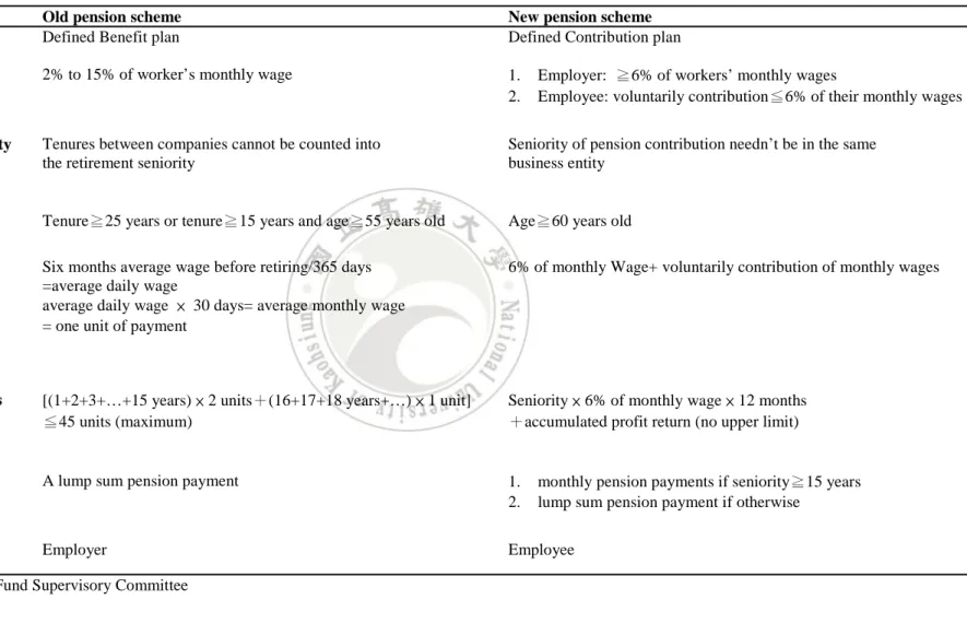
(11) government (65% of the monthly contribution) and the public-sector workers (35% of the monthly contribution). A Public-sector worker whose tenure is over than 25 years, or the tenure is more than 5 years and older than 60 years old is eligible to claim the pension. On the other hand, the private-sector pension administered by the Bureau of Labor Insurance was implemented under the DB plan in 1984. Under the DB plan, employer is required, but not strongly forced by the government, to contribute 2% to 15% of worker’s monthly wage to the retirement reserve fund. A private-sector worker who works in a company for more than 25 years, or over 15 years and older than 55 is eligible to claim the pension. Until the end of 2003, only 55,277 companies (14.14%) in Taiwan have contributed to the retirement reverse fund and most of them are large enterprises (Council of Labor Affairs, 2003). Since the DB plan has been implemented, only 20 percent of the retired private-sector workers received pension and half of them received less than $500,000 NT dollars ($17,000 US dollar) in lump-sum. To provide financial security for the private-sector workers and improved the labor market efficiency, government replaced the DB plan with the DC plan in July 2005. Under the DC plan, the contribution may be made by the employer and/or the workers. Employer is required regularly contribute at least 6% of worker’s monthly wages to their personal retirement account and the ownership of the account belongs to worker. Employee also can voluntarily contribute at most 6% of their monthly wages. A worker who is older than 60 years old is eligible to claim the pension and can choose to receive their pension in lump-sum or monthly payment. A pension comparison of old and new pension scheme is shown in Table 1. During the transition period, workers can choose whether to enroll in DC plan or stay with the DB plan within five years after implementation date except for those. 6.

(12) Table 1. Comparison of old and new pension schemes System. Old pension scheme Defined Benefit plan. New pension scheme Defined Contribution plan. Contribution rate. 2% to 15% of worker’s monthly wage. 1. 2.. Calculation of seniority. Tenures between companies cannot be counted into the retirement seniority. Seniority of pension contribution needn’t be in the same business entity. Claim. Tenure≧25 years or tenure≧15 years and age≧55 years old. Age≧60 years old. Unit of payment. Six months average wage before retiring/365 days =average daily wage average daily wage × 30 days= average monthly wage = one unit of payment. 6% of monthly Wage+ voluntarily contribution of monthly wages. Standard of payments. [(1+2+3+…+15 years) × 2 units＋(16+17+18 years+…) × 1 unit] ≦45 units (maximum). Seniority × 6% of monthly wage × 12 months ＋accumulated profit return (no upper limit). Type of payments. A lump sum pension payment. 1. 2.. Ownership. Employer. Employee. Source: Labor Pension Fund Supervisory Committee. 7. Employer: ≧6% of workers’ monthly wages Employee: voluntarily contribution≦6% of their monthly wages. monthly pension payments if seniority≧15 years lump sum pension payment if otherwise.

(13) who just enter the labor market or change jobs. By the end of 2010, there are 5,482,848 (87.14%) workers enrolled in new pension scheme and 406,526 business entities (94.05%) allocate workers’ pension (Council of Labor Affairs, 2010). III. Empirical Strategies The 2005 pension reform gives rise to a natural experiment that allows us separating the sample into comparison and treatment groups and use DD and DDD approach to examine the effect of the pension reform on mobility and wage. Since the 2005 pension reform affects private-sector workers only, we treat private-sector worker and public-sector worker as the treatment and comparison group, respectively. III.A. Difference-in-Differences estimates We use two measures of mobility in the analysis. The first one is Mover which equals one if a worker whose tenure was less than 17 months and had changed jobs at least once last year or was voluntarily unemployed for less than 17 months and had worked prior to being unemployed, and zero otherwise. We use 17 months as the cutoff point because the MUS collects information in May every years. If a worker changed job last year, we will observe that his/her tenure is less than 17 months. The second one is Tenure, which is defined as the number of years at current job. The model takes the following form: 𝑀𝑝𝑝𝑎𝑝 = 𝛽0 + 𝛽1(𝑝𝑝𝑝𝑝2005 × 𝑝𝑝𝑝𝑝) + 𝛽2 𝑝𝑝𝑝𝑝 + 𝛽3 𝑝𝑝𝑝𝑝2005 + 𝛽4 𝑎𝑎𝑎 +𝛽5 𝑎𝑎𝑎2 + 𝛽6 𝑤_𝑐𝑐𝑐𝑐𝑐𝑐 + 𝛽7 (𝑝𝑝𝑝𝑝 × 𝑠ℎ𝑜𝑜𝑜𝑜𝑜𝑜) + 𝛽8 𝑢𝑢𝑢𝑢𝑢 +𝛽9(𝑦𝑦2004 × 𝑝𝑝𝑝𝑝) + 𝛾′𝑍i + 𝑢i. (2). where priv is an indicator of private-sector worker. We classify sectors by workers previous job. For stayers, they do not have pervious job data, so we classify sectors by their current job which is also their job 17 months ago, post2005 is a dummy variable identifying the years after the implementation of new pension policy, age and age2 8.

(14) are age and age square, w_collar is an indicator of white collar workers, shortage is an indicator of labor shortage rate which is calculated by dividing the numbers of work shortage by the numbers of work shortage plus the numbers of work employment and then times 100. The data of average shortage rate is merged with MUS by year and industry. In general, the public-sector labor shortage rate in Taiwan is very close to zero because the numbers of people who wants to get into the public sector is always greater than the numbers of job offer by public sector. As a result, we assume the public-sector labor shortage rate equals to zero and replace shortage with priv×shortage for estimation, urate is the unemployment rate in the county of residence, yr2004 is a dummy variable for year 2004 and the interaction term of yr2004×priv captures the different time trend between private- and public-sector workers in the per-policy period. The DD model is based on the assumption that apart from the exogenous variables, the time trend of the dependent variable should follow parallel paths when the treatment is absent. Hence, we use yr2004×priv to see whether there is a common trend of mobility between the treatment and comparison groups in the per-policy period, Z is a vector of demographic variables that includes individuals’ year of schooling, marital status, work location, industry and year dummies. The DD estimate is the coefficient of post2005×pirv, representing the effect of pension reform on the mobility of private-sector workers as opposed to public-sector workers over the period of the reform. We estimate Tenure equation with the same specification of equation (2) and include the current firm size dummies and logarithm of real hourly wage: 𝑇𝑎𝑙𝑢𝑝𝑎 = 𝛽0 + 𝛽1(𝑝𝑝𝑝𝑝2005 × 𝑝𝑝𝑝𝑝) + 𝛽2 𝑝𝑝𝑝𝑝 + 𝛽3 𝑝𝑝𝑝𝑝2005 + 𝛽4 𝑎𝑎𝑎 +𝛽5 𝑎𝑎𝑎2 + 𝛽6 𝑙𝑙𝑙 + 𝛽7 𝑤_𝑐𝑐𝑐𝑐𝑐𝑐 + 𝛽8 (𝑝𝑝𝑝𝑝 × 𝑠ℎ𝑜𝑜𝑜𝑜𝑜𝑜) 9. (3).

(15) +𝛽9 𝑢𝑢𝑢𝑢𝑢 + 𝛽10 (𝑝𝑝𝑝𝑝 × 𝑠𝑠𝑠𝑠𝑠) + 𝛽11 (𝑝𝑝𝑝𝑝 × 𝑙𝑙𝑙𝑙𝑙) +𝛽12(𝑦𝑦2004 × 𝑝𝑝𝑝𝑝) + 𝛾′𝜃i + 𝑢i. where priv is an indicator of private-sector worker. In Tenure equation, we want to estimate how the 2005 reform affects worker’s tenure in their current company. As a result, we classify sectors by worker’s current job, lnw is the logarithm of real hourly wage, which is calculated by dividing monthly wages by hours worked per month and then is adjusted by CPI (the base year is 2005), small is an indicator of small firm which has less than 100 employees, large is an indicator of large firm which has more than 500 employees. Since the current job firm size is collected only for private-sector workers, we replace current firm size dummies (small and large) with the interaction term of priv×small and priv×large in Tenure equation. The reasons why we do not include the current firm size dummy in Mover equation is that the pervious firm size was collected only for movers who have three months work experiences before current job, 𝜃 is a vector of demographic variables that includes individuals’ year of. schooling, marital status, work location, industry and year dummies.. III.B. Difference-in-Difference-in-Differences Estimates The unobserved heterogeneity between private- and public-sector workers may contaminate our estimates of mobility. We create an additional control group and use DDD model to fix this problem. Given that workers whose tenure is 15 years or over should have no incentive to switch to the DC plan, they can serve as an additional control group. III.B.1. The effect of pension reform on mobility Given that tenure is used to define the dependent variable of Mover and Tenure, we use age to construct this additional control group. In our data, the average tenure for workers whose age is over 45, 50 and 55 years old is 12.67, 13.99, and 14.03 years, 10.

(16) respectively. In addition, the percentage of worker whose tenure is at least 15 years is 40.16%, 44.94%, and 47.19% among three age groups. This shows that using age as an indicator for the additional control group may not cause significant bias. Hence, we use ages 45, 50 and 55 as the cutoff points for sensitivity checks. The model takes the following form: 𝑀𝑝𝑝𝑎𝑝 = 𝛽0 + 𝛽1(𝑝𝑝𝑝𝑝2005 × 𝑝𝑝𝑝𝑝 × 𝑦𝑦𝑦𝑦𝑦) + 𝛽2 𝑝𝑝𝑝𝑝 + 𝛽3 𝑝𝑝𝑝𝑝2005 +𝛽4 𝑦𝑦𝑦𝑦𝑦 + 𝛽5 (𝑝𝑝𝑝𝑝2005 × 𝑝𝑝𝑝𝑝) + 𝛽6 (𝑝𝑝𝑝𝑝 × 𝑦𝑦𝑦𝑦𝑦). (4). +𝛽7 (𝑝𝑝𝑝𝑝2005 × 𝑦𝑦𝑦𝑦𝑦) + 𝛽8 𝑤_𝑐𝑐𝑐𝑐𝑐𝑐 + 𝛽9 (𝑝𝑝𝑝𝑝 × 𝑠ℎ𝑜𝑜𝑜𝑜𝑜𝑜) +𝛽10 𝑢𝑢𝑢𝑢𝑢 + 𝛽11(𝑦𝑦2004 × 𝑝𝑝𝑝𝑝) + 𝛿′𝑅i + 𝑒i. where young equals one if age is less than the cutoff ages, and zero otherwise; R includes individuals’ year of schooling, marital status, work location, industry and year dummies. We estimate Tenure equation with the same specification of equation (4) and include lnw and the interaction terms of priv×small and priv×large in the regression. The DDD estimate is the coefficient of post2005×priv×young, representing the impact of pension reform on the mobility decision of young private-sector workers as opposed to their old public-sector counterparts. We estimate Mover equation by linear probability model (LPM) and estimate Tenure equation by OLS. III.B.2. The impact of pension reform on wages To compare our results with those reported in Luoh and Yang (2009), we use DDD approach to estimate the effect of 2005 reform on wages. In Luoh and Yang’s paper, they use data from the MUS 2003-2007 and focus on full-time workers (hours worked at least 40 per week) whose wage is greater than minimum wage ($15,840). They also limit the sample to young workers, whose tenure is less than two years in pre-policy and post-policy periods. On the other hand, we extend the time period to ten years 11.

(17) (2000-2010) and restrict our sample to non-agricultural full time workers (hours worked at least 35 per week) to estimate the following regression by OLS model: 𝑐𝑙𝑤 = 𝛽0 + 𝛽1 (𝑝𝑝𝑝𝑝2005 × 𝑝𝑝𝑝𝑝 × 𝑦𝑦𝑦𝑦𝑦) + 𝛽2 𝑝𝑝𝑝𝑝 + 𝛽3 𝑝𝑝𝑝𝑝2005 +𝛽4 𝑦𝑦𝑦𝑦𝑦 + 𝛽5 (𝑝𝑝𝑝𝑝2005 × 𝑝𝑝𝑝𝑝) + 𝛽6 (𝑝𝑝𝑝𝑝 × 𝑦𝑦𝑦𝑦𝑦). (5). +𝛽7 (𝑝𝑝𝑝𝑝2005 × 𝑦𝑦𝑦𝑦𝑦) + 𝛽8 (yr2004 × priv) + 𝜃′𝑋i + 𝜐i. where lnw is the logarithm of real hourly wage; young equals to one if tenure is less than 10, 15,20, respectively, for sensitivity check, X includes individuals’ age, year of schooling, marital status, work place, current firm size, industry and year dummies. We use tenure as the measurement of young worker because there is no correlation between tenure and wages in Wage equation. To account for the potential bias caused by repeated cross-sections of individual data, the standard errors are cluster at household ID for Mover, Tenure and Wage equations. IV. Data The data in our study are from the Manpower Utilization Survey (MUS) 2000-2010, which represents repeated cross-sections with different individuals in each survey. The MUS is conducted by Taiwan’s Directorate -General of Budget, Accounting, and Statistics in May every year since 1978. All persons aged 15 and over in the household were interviewed. The MUS collects information on employment status, demographic characteristics, occupation, industry, firm size, monthly wages, tenure, and work history. We restrict our sample to non-agricultural full-time (hours worked more than 35) workers aged between 26 and 60. The age restriction is to eliminate those just entering the labor market or retiring. People served in the armed forces are also excluded. We use data from 2000-2004 and 2006-2010 representing the pre-policy and post-policy periods, respectively, and drop the transition year 2005. The final 12.

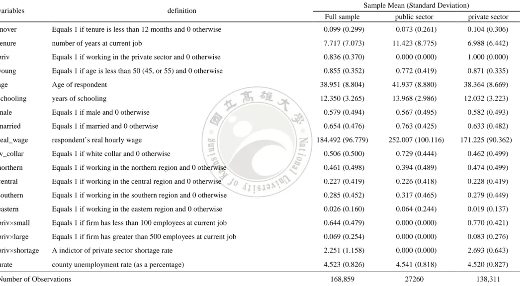
(18) sample consists of 168,859 respondents. Table 2 shows the definitions and descriptive statistics of the variables by sector. Nearly ten percent of the sample changed job last year. The mean tenure for all individuals is 7.17 years. The mean tenure for public-sector workers is 11.42 years. The mean tenure for private-sector workers is 6.98 years. 83.6% of the individuals work in the private sector. The mean age of all respondents is 38.95 years old. The average age of public-sector workers is three years older than private-sector workers. The average year of schooling is 12.35 in the full sample. Fifty-eight of respondents are male. 64.5% of individuals are married. Comparing with public-sector workers, the percentage of mover is higher for private-sector workers. 10.4% of private-sector workers changed job last year. The mean tenure of private-sector workers is 4.43 years (11.42-6.99) shorter than public-sector workers. The percentage of young worker (age<50) in the public and private sectors are 77.2% and 87.1%, respectively. The average age for public-sector workers is 41.93 years old and 38.36 years old for private-sector workers. The mean year of schooling for public-sector workers is one year more than private-sector workers. The mean real hourly wage is NT $252.01 (US $8.44) which is 1.47 times more than private-sector workers (NT $171.23 or US $5.73). The percentage of white collar workers is 72.9% and 46.2% in public and private sector, respectively. In full sample, 46.1% of the respondents work in northern Taiwan. 77% of private-sector workers are in the small firms whereas only 8.3% of them work in the large firms. For the estimation of Mover equation, we also include those who are voluntarily unemployed for less than 17 months and had worked prior to being unemployed as movers. In addition, we drop those who did not work at least three months prior to current job because their work history was not collected and they are likely to be just 13.

(19) Table 2. Definitions of Variables, sample means, and standard deviation: 2000-2010 variables. Sample Mean (Standard Deviation). definition. Full sample. public sector. private sector. mover. Equals 1 if tenure is less than 12 months and 0 otherwise. 0.099 (0.299). 0.073 (0.261). 0.104 (0.306). tenure. number of years at current job. 7.717 (7.073). 11.423 (8.775). 6.988 (6.442). priv. Equals 1 if working in the private sector and 0 otherwise. 0.836 (0.370). 0.000 (0.000). 1.000 (0.000). young. Equals 1 if age is less than 50 (45, or 55) and 0 otherwise. 0.855 (0.352). 0.772 (0.419). 0.871 (0.335). age. Age of respondent. 38.951 (8.804). 41.937 (8.880). 38.364 (8.669). schooling. years of schooling. 12.350 (3.265). 13.968 (2.986). 12.032 (3.223). male. Equals 1 if male and 0 otherwise. 0.579 (0.494). 0.567 (0.495). 0.582 (0.493). married. Equals 1 if married and 0 otherwise. 0.654 (0.476). 0.763 (0.425). 0.633 (0.482). real_wage. respondent’s real hourly wage. 184.492 (96.779). 252.007 (100.116). 171.225 (90.362). w_collar. Equals 1 if white collar and 0 otherwise. 0.506 (0.500). 0.729 (0.444). 0.462 (0.499). northern. Equals 1 if working in the northern region and 0 otherwise. 0.461 (0.498). 0.394 (0.489). 0.474 (0.499). central. Equals 1 if working in the central region and 0 otherwise. 0.227 (0.419). 0.226 (0.418). 0.228 (0.419). southern. Equals 1 if working in the southern region and 0 otherwise. 0.285 (0.452). 0.317 (0.465). 0.279 (0.449). eastern. Equals 1 if working in the eastern region and 0 otherwise. 0.026 (0.160). 0.064 (0.244). 0.019 (0.137). priv×small. Equals 1 if firm has less than 100 employees at current job. 0.644 (0.479). 0.000 (0.000). 0.770 (0.421). priv×large. Equals 1 if firm has greater than 500 employees at current job. 0.069 (0.254). 0.000 (0.000). 0.083 (0.276). priv×shortage. A indictor of private sector shortage rate. 2.251 (1.158). 0.000 (0.000). 2.693 (0.643). urate. county unemployment rate (as a percentage). 4.523 (0.826). 4.541 (0.818). 4.520 (0.827). 168,859. 27260. 138,311. Number of Observations Notes: Standard deviations are in parentheses. 14.

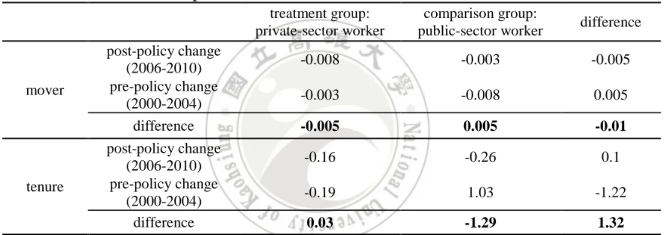
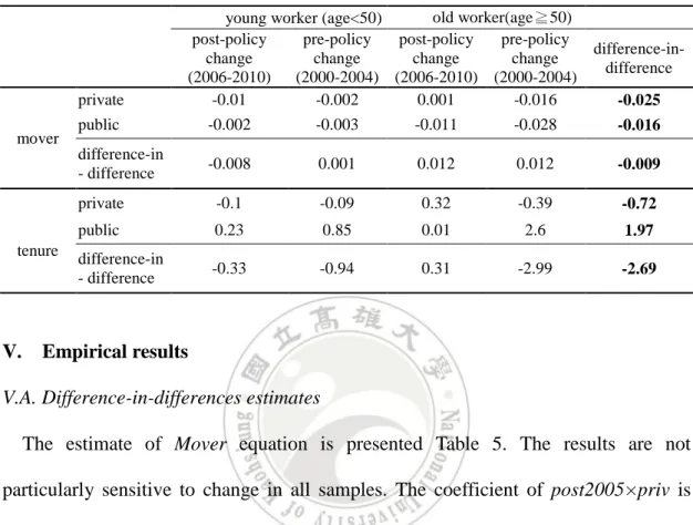
(20) entering the job market. After the restrictions, the sample consists of 168,064 respondents. We first calculate the simple DD estimate of treatment effect by using the following equation: ∆yi = [(yi|private, post2005) − (yi|private, pre2005)] − [(yi|public, post2005) − (yi|public, pre2005)]. Table 3 shows that the difference in the changes of the percentage of mover and tenure between private and public sector is -0.01 and 1.32, respectively. The results suggest that the 2005 pension reform may not reduce the job-lock effect. Table 3. The result of simple DD estimate of treatment effect. mover. tenure. post-policy change (2006-2010) pre-policy change (2000-2004) difference post-policy change (2006-2010) pre-policy change (2000-2004) difference. treatment group: private-sector worker. comparison group: public-sector worker. difference. -0.008. -0.003. -0.005. -0.003. -0.008. 0.005. -0.005. 0.005. -0.01. -0.16. -0.26. 0.1. -0.19. 1.03. -1.22. 0.03. -1.29. 1.32. We also calculate the simple DDD estimate of treatment effect by using the following equation: ∆yi = {[(young, post2005) − (young, pre2005)|private] −[(old, post2005) − (old, pre2005)|private]}. −{[(young, post2005) − (young, pre2005)|public] −[(old, post2005) − (old, pre2005)|public]. We use young workers whose age is less than 50 as an example to calculate the simple DDD estimate. In Table 4, the difference in the changes of the percentage of mover is -0.009 and in the changes of tenure is -2.69 between young private-sector 15.

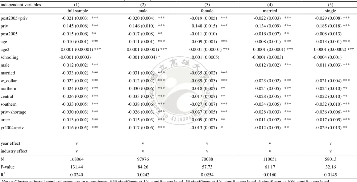
(21) workers and their counterparts after 2005. The simple DDD estimate shows that the effect of the 2005 reform on mobility is mixed. To confirm that the 2005 reform has effect on mobility, we need to control other variables that might affect mobility. Table 4. The result of simple DDD estimate of treatment effect. private mover. tenure. V.. old worker(age≧50) young worker (age<50) post-policy pre-policy post-policy pre-policy change change change change (2006-2010) (2000-2004) (2006-2010) (2000-2004) -0.01 -0.002 0.001 -0.016. difference-indifference -0.025. public. -0.002. -0.003. -0.011. -0.028. -0.016. difference-in - difference. -0.008. 0.001. 0.012. 0.012. -0.009. private. -0.1. -0.09. 0.32. -0.39. -0.72. public. 0.23. 0.85. 0.01. 2.6. 1.97. difference-in - difference. -0.33. -0.94. 0.31. -2.99. -2.69. Empirical results. V.A. Difference-in-differences estimates The estimate of Mover equation is presented Table 5. The results are not particularly sensitive to change in all samples. The coefficient of post2005×priv is negative and statistically significant in all samples. The mobility probability for private-sector workers decreases by 0.021 percentage point after 2005 in full sample and decreases by 0.02, 0.019, 0.022, and 0.029 percentage points in male, female, married and single samples, respectively. The coefficient of priv indicates that the mobility probability of private-sector workers are 0.145, 0.146, 0.148, 0.134 and 0.185 percentage points greater than public-sector workers in full, male, female, married and single samples, respectively. After 2005, the mobility probability decreases by 0.015 percentage point in full sample. The negative sign of post2005×priv suggests that the pension portability dose not reduce the job-lock effect. Our finding is consistent with what Gustman and Steinmerier (1993) and 16.

(22) Table 5. Difference-in-Difference Estimates of Mobility Probability, 2000-2010 independent variables post2005×priv priv. (1) full sample. (2) male. (3) female. (4) married. (5) single. -0.021 (0.003) ***. -0.020 (0.004) ***. -0.019 (0.005) ***. -0.022 (0.003) ***. -0.029 (0.008) ***. 0.145 (0.008) ***. 0.146 (0.010) ***. 0.148 (0.015) ***. 0.134 (0.009) ***. 0.185 (0.018) ***. post2005. -0.015 (0.006) **. -0.017 (0.008) **. -0.011 (0.010). -0.016 (0.007) **. -0.008 (0.013). age. -0.010 (0.001) ***. -0.011 (0.001) ***. -0.009 (0.001) ***. -0.008 (0.001) ***. -0.013 (0.001) ***. age2. 0.0001 (0.00001) ***. 0.0001 (0.00001) ***. 0.0001 (0.00001) ***. 0.0001 (0.00001) ***. 0.0001 (0.00002) ***. schooling male. -0.0001 (0.0003). -0.001 (0.0004) *. 0.001 (0.0005). 0.012 (0.002) ***. -0.0001 (0.0003). -0.0004 (0.001). 0.012 (0.002) ***. 0.011 (0.003) ***. married. -0.033 (0.002) ***. -0.031 (0.002) ***. -0.035 (0.002) ***. w_collar. -0.022 (0.002) ***. -0.012 (0.002) ***. -0.039 (0.003) ***. -0.023 (0.002) ***. -0.021 (0.004) ***. northern. -0.024 (0.005) ***. -0.030 (0.006) ***. -0.018 (0.007) **. -0.024 (0.005) ***. -0.024 (0.010) **. central. -0.026 (0.005) ***. -0.033 (0.007) ***. -0.017 (0.007) **. -0.028 (0.005) ***. -0.022 (0.010) **. southern. -0.033 (0.005) ***. -0.038 (0.006) ***. -0.027 (0.007) ***. -0.034 (0.005) ***. -0.032 (0.010) ***. priv×shortage. -0.030 (0.003) ***. -0.026 (0.003) ***. -0.037 (0.005) ***. -0.028 (0.003) ***. -0.036 (0.006) ***. 0.013 (0.002) ***. 0.015 (0.003) ***. 0.009 (0.003) **. 0.011 (0.002) ***. 0.017 (0.005) ***. -0.016 (0.005) ***. -0.017 (0.006) ***. urate yr2004×priv. -0.013 (0.007) *. -0.012 (0.005) **. -0.029 (0.013) **. year effect. v. v. v. v. v. industry effect. v. v. v. v. v. N. 168064. 97976. 70088. 110051. 58013. F-value. 131.44. 84.26. 57.73. 61.17. 32.16. 0.0240. 0.0242. 0.0254. 0.0160. 0.0145. 2. R. Notes: Cluster-adjusted standard errors are in parentheses. *** significant at 1% significance level. ** significant at 5% significance level. * significant at 10% significance level 17.

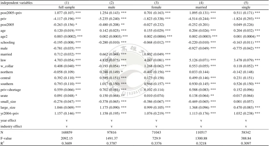
(23) Andrietti and Hildebrand (2001) found. These studies suggest that the pension covered jobs often offer better compensations and benefits (such as health insurance or union). It is these benefits that account for lower mobility rather than the non-portability. Unfortunately, we do not have company compensation information in our data and all Taiwanese are covered by National Health Insurance (NHI). We are unable to examine whether the provision of compensations and benefits are worker’s main consideration for changing jobs. In addition, our method of classification may not reflect the true mobility of a worker. In our data, there is no specific question asking whether workers changed job last year. We only can use tenure less than 17 months as cutoff point and changing work location more than once last year when definition of a mover. The remainder of the variables generally has the expected signs. Based on the column (1), one year increase in age decreases the mobility probability by 0.01 percentage point. One year increase in schooling decreases the mobility probability by 0.0001 percentage point but the reduction is insignificant. Males are more likely to change job than females. Married workers have lower mobility probability than single workers. The white collar workers are 0.022 less likely to change jobs than blue collar workers. The mobility probability significantly decreases by 0.03 percentage point when labor shortage rate increases by one percent. One percent increase in county unemployment rate increases the mobility probability by 0.013. The coefficient of yr2004×priv is negative and statistically significant, which indicates that the mobility probability for private-sector workers is 0.016 percentage point lower than public-sector workers in 2004 (the pre-policy period). Table 6 reports the results for Tenure. The tenure of private-sector workers significantly increases by 1.08, 1.25, 0.7, 1.09, and 0.51 years after 2005 in full, male, 18.

(24) Table 6. Difference-in-Difference Estimate of Tenure, 2000-2010 independent variables post2005×priv. (1) full sample. (2) male. (3) female. (4) married. (5) single. 1.077 (0.107) ***. 1.254 (0.143) ***. 0.701 (0.163) ***. 1.095 (0.131) ***. 0.511 (0.171) ***. priv. -4.117 (0.196) ***. -5.235 (0.240) ***. -1.823 (0.338) ***. -4.514 (0.244) ***. -1.824 (0.293) ***. post2005. -0.263 (0.156) *. -0.480 (0.208) **. -0.027 (0.232). -0.252 (0.201). 0.049 (0.226). age. 0.120 (0.019) ***. 0.142 (0.025) ***. 0.155 (0.029) ***. 0.204 (0.026) ***. 0.204 (0.032) ***. age2. 0.003 (0.0002) ***. 0.002 (0.0003) ***. 0.002 (0.0004) ***. 0.002 (0.0003) ***. 0.001 (0.0004) **. schooling. -0.195 (0.008) ***. male. -0.781 (0.035) ***. -0.280 (0.010) ***. -0.068 (0.012) ***. -0.220 (0.010) ***. -0.163 (0.011) ***. -0.927 (0.049) ***. -0.775 (0.042) ***. married. 0.712 (0.032) ***. 0.662 (0.044) ***. 0.802 (0.049) ***. lnw. 4.703 (0.054) ***. 4.835 (0.075) ***. 4.247 (0.081) ***. 5.126 (0.071) ***. 3.478 (0.079) ***. w_collar. 0.408 (0.040) ***. -0.193 (0.054) ***. 1.268 (0.062) ***. 0.553 (0.055) ***. 0.118 (0.052) **. northern. -0.058 (0.109). 0.288 (0.149) *. -0.407 (0.156) ***. 0.033 (0.144). -0.142 (0.148). central. 0.392 (0.110) ***. 0.589 (0.151) ***. 0.173 (0.158). 0.499 (0.146) ***. 0.231 (0.151). southern. 0.793 (0.110) ***. 1.017 (0.150) ***. 0.566 (0.157) ***. 0.930 (0.145) ***. 0.526 (0.150) ***. priv×shortage. 0.559 (0.066) ***. 0.702 (0.081) ***. 0.102 (0.114). 0.588 (0.083) ***. 0.152 (0.096). urate. 0.091 (0.048) *. 0.150 (0.064) **. 0.010 (0.074). 0.138 (0.064) **. -0.017 (0.064) 0.001 (0.057). small_size. -0.276 (0.047) ***. -0.378 (0.065) ***. -0.386 (0.067) ***. -0.469 (0.065) ***. large_size. 1.046 (0.069) ***. 1.175 (0.090) ***. 0.999 (0.105) ***. 1.368 (0.096) ***. 0.470 (0.083) ***. yr2004×priv. 1.157 (0.146) ***. 1.158 (0.195) ***. 1.076 (0.219) ***. 1.113 (0.176) ***. 1.032 (0.238) ***. year effect. v. v. v. v. v. industry effect. v. v. v. v. v. 168859. 97816. 71043. 110517. 58342. N. F-value 2092.15 1491.37 729.9 1300.88 388.84 R2 0.3609 0.3787 0.3376 0.3218 0.3097 Notes: Cluster-adjusted standard errors are in parentheses. *** significant at 1% significance level. ** significant at 5% significance level. * significant at 10% significance level 19.

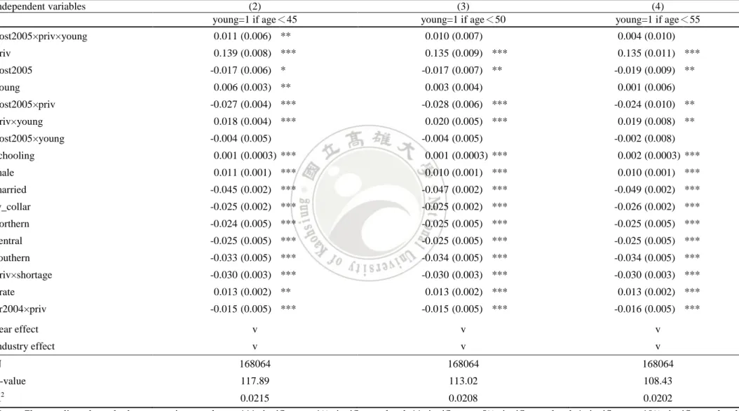
(25) female, married and single samples, respectively. The tenure of private-sector workers is 4.12 years shorter than that of public-sector workers in full sample. After 2005, the tenure significantly decreases by 0.26 and 0.48 in full and male samples, respectively. Consequently, the positive sign of post2005×priv indicates that the 2005 pension reform does not make workers leave their current job, but make workers stay longer in their current job instead. The result suggests that the 2005 reform may not reduce the job-lock effect. Other variables have the expected sign. Based on the column (1), age has a positive effect on tenure. One year increase in age increases the tenure by 0.12 years. One year increase in schooling decreases the tenure by 0.195 years. Male’s tenure is 0.78 years shorter than female’s. Being married are positively related to tenure. One percent increase in wage increases the tenure by 4.7 years. The tenure significantly increases by 0.56 years when labor shortage rate increases by one percent but the effect is insignificant in female and single samples. When the county unemployment rate increases by one percent, the worker’s tenure will increase by 0.09 years. Workers in the large company will stay longer than those in the small company. The interaction of yr2004×priv is positive which indicates that the tenure of private-sector worker is 1.57 years longer than public-sector workers in 2004 (per-policy period).. V.B. Difference-in-difference-in-differences estimates V.B.1. The effect of pension reform on mobility Table 7 shows the DDD estimate of Mover equation. The results are not particularly sensitive to change in three age groups. The coefficient of post2005×priv×younger shows that the pension reform has a significant positive effect on mobility probability for young worker in 45 age group, but insignificant in 50 and 55 age group. The mobility probability increases by 0.011 percentage points for young (45 age group) 20.

(26) Table 7. Difference-in-Difference-in-Differences Estimate of Mobility Probability, 2000-2010 independent variables. (2) young=1 if age＜45. post2005×priv×young. 0.011 (0.006) **. 0.010 (0.007). 0.004 (0.010). priv. 0.139 (0.008) ***. 0.135 (0.009) ***. 0.135 (0.011) ***. post2005 young post2005×priv priv×young post2005×young. (3) young=1 if age＜50. -0.017 (0.006) *. -0.017 (0.007) **. 0.006 (0.003) **. 0.003 (0.004). (4) young=1 if age＜55. -0.019 (0.009) ** 0.001 (0.006). -0.027 (0.004) ***. -0.028 (0.006) ***. -0.024 (0.010) **. 0.018 (0.004) ***. 0.020 (0.005) ***. 0.019 (0.008) **. -0.004 (0.005). -0.004 (0.005). -0.002 (0.008). schooling. 0.001 (0.0003) ***. 0.001 (0.0003) ***. 0.002 (0.0003) ***. male. 0.011 (0.001) ***. 0.010 (0.001) ***. 0.010 (0.001) ***. married. -0.045 (0.002) ***. -0.047 (0.002) ***. -0.049 (0.002) ***. w_collar. -0.025 (0.002) ***. -0.025 (0.002) ***. -0.026 (0.002) ***. northern. -0.024 (0.005) ***. -0.025 (0.005) ***. -0.025 (0.005) ***. central. -0.025 (0.005) ***. -0.025 (0.005) ***. -0.025 (0.005) ***. southern. -0.033 (0.005) ***. -0.034 (0.005) ***. -0.034 (0.005) ***. priv×shortage. -0.030 (0.003) ***. -0.030 (0.003) ***. -0.030 (0.003) ***. 0.013 (0.002) **. 0.013 (0.002) ***. 0.013 (0.002) ***. -0.015 (0.005) ***. -0.015 (0.005) ***. -0.016 (0.005) ***. year effect. v. v. v. industry effect. v. v. v. N. 168064. 168064. 168064. F-value. 117.89. 113.02. 108.43. 0.0215. 0.0208. 0.0202. urate yr2004×priv. 2. R. Notes: Cluster-adjusted standard errors are in parentheses. *** significant at 1% significance level. ** significant at 5% significance level. * significant at 10% significance level 21.

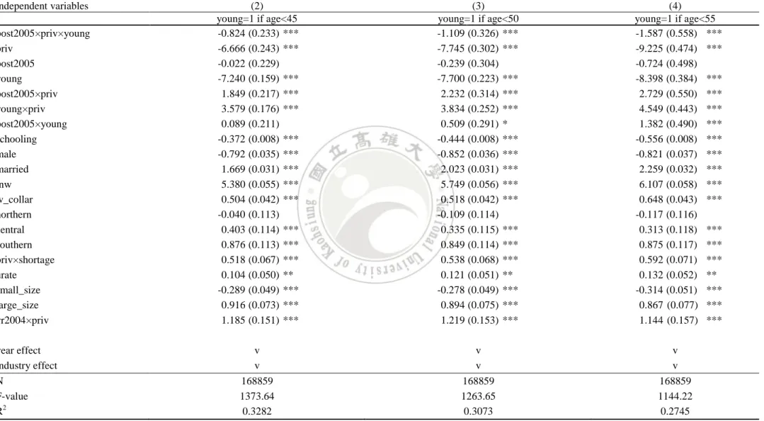
(27) private-sector workers after 2005 reform. These results are opposite to Table 5 and suggest that the 2005 pension reform may reduce the job-lock effect. In addition, the mobility probability of young private-sector workers increases by 0.14 percentage point across three age groups. After 2005, the mobility probability decreases by 0.017 percentage point in 45 age group. Young workers (age<45) are more likely to change job. Based on column (1), the interaction term of post2005×priv indicates that the private-sector worker is 0.027 less likely to change jobs than public-sector worker after 2005. The young private-sector workers are 0.018 more likely to change jobs than their counterparts. The coefficient of post2005×young suggests that the young workers are 0.004 less likely to change jobs than old workers after 2005 but it is insignificant at any level. One year increase in schooling significantly increases the mobility probability by 0.001. The reminder variables have the same signs and similar magnitude comparing to the DD results. In Table 8 reports the DDD estimate of Tenure equation. The coefficient of post2005×priv×young is negative and statistically significant across three age groups. The tenure of young private-sector workers reduces by 0.82, 1.11, and 1.59 years in three age groups after 2005 reform, respectively. These results are contrary to those in Table 6. Our results support the hypothesis that the 2005 pension reform significantly decreases the tenure for young private-sector workers as opposed to that for their counterparts. Based on column (2), the tenure of private-sector worker is 7.75 years shorter than public-sector worker’s. After 2005 reform, worker’s tenure reduces by 0.24 years but it is not statistically significant. The tenure of young workers is 7.7 years shorter than old workers. The interaction term of post2005×priv suggests that the tenure of private-sector workers is 2.23 years longer than public-sector workers after 2005. The tenure of young private-sector workers is 3.83 years longer than their 22.

(28) Table 8. Difference-in-Difference-in-Differences Estimate of Tenure, 2000-2010 independent variables post2005×priv×young priv post2005 young post2005×priv young×priv post2005×young schooling male married lnw w_collar northern central southern priv×shortage urate small_size large_size yr2004×priv. (2) young=1 if age<45 -0.824 (0.233) *** -6.666 (0.243) *** -0.022 (0.229) -7.240 (0.159) *** 1.849 (0.217) *** 3.579 (0.176) *** 0.089 (0.211) -0.372 (0.008) *** -0.792 (0.035) *** 1.669 (0.031) *** 5.380 (0.055) *** 0.504 (0.042) *** -0.040 (0.113) 0.403 (0.114) *** 0.876 (0.113) *** 0.518 (0.067) *** 0.104 (0.050) ** -0.289 (0.049) *** 0.916 (0.073) *** 1.185 (0.151) ***. (3) young=1 if age<50 -1.109 (0.326) *** -7.745 (0.302) *** -0.239 (0.304) -7.700 (0.223) *** 2.232 (0.314) *** 3.834 (0.252) *** 0.509 (0.291) * -0.444 (0.008) *** -0.852 (0.036) *** 2.023 (0.031) *** 5.749 (0.056) *** 0.518 (0.042) *** -0.109 (0.114) 0.335 (0.115) *** 0.849 (0.114) *** 0.538 (0.068) *** 0.121 (0.051) ** -0.278 (0.049) *** 0.894 (0.075) *** 1.219 (0.153) ***. (4) young=1 if age<55 -1.587 (0.558) *** -9.225 (0.474) *** -0.724 (0.498) -8.398 (0.384) *** 2.729 (0.550) *** 4.549 (0.443) *** 1.382 (0.490) *** -0.556 (0.008) *** -0.821 (0.037) *** 2.259 (0.032) *** 6.107 (0.058) *** 0.648 (0.043) *** -0.117 (0.116) 0.313 (0.118) *** 0.875 (0.117) *** 0.592 (0.071) *** 0.132 (0.052) ** -0.314 (0.051) *** 0.867 (0.077) *** 1.144 (0.157) ***. year effect v v v industry effect v v v N 168859 168859 168859 F-value 1373.64 1263.65 1144.22 R2 0.3282 0.3073 0.2745 Notes: Cluster-adjusted standard errors are in parentheses. *** significant at 1% significance level. ** significant at 5% significance level. * significant at 10% significance level 23.

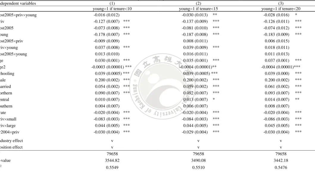
(29) counterparts. In addition, the tenure of young workers is 0.51 years longer than old workers after 2005. Other variables have the expected sign. Based on the column (2), education has negative effect on tenure. One year increase in schooling decreases the tenure by 0.44 years. Male’s tenure is 0.85 years shorter than female’s. Being married are positively related to tenure. One percent increase in wage increases the tenure by 5.75 years. One percent increase in labor shortage increases the tenure by 0.54 years. County unemployment rate has a positive effect on tenure. Workers in large companies will stay 0.89 years longer than those in small companies. The coefficient of yr2004×priv is positive, which shows that the tenure of private-sector workers is 1.22 years longer than public-sector workers in 2004 (per-policy period). V.B.2. The effect of pension reform on wage Table 9 reports the DDD estimate of Wage equation. The results show that the 2005 reform has a negative effect on wages. The coefficient of post2005×priv×young indicates that pension reform significantly reduces worker’s wage by 3% when young worker is defined as tenure less than 15 years. When young worker is defined as tenure less than 20 years, the wage decrease by 2.8% and remains significant at the 10 percent level. Unlike Luoh and Yang (2009), who find that employer can shift all the increased costs due to reform to the workers, our result suggests that only half of the increased costs are shifted to workers. Vestad (2011) and Sheu and Lee (2012) reach the similar conclusions to yours. Vestad (2011) shows that less than 50% of the cost of a minimum pension contribution is shifted from the company to workers. Sheu and Lee (2012) find that the 2005 reform has a negative effect on wages which reduce by 1.92%. Based on the column (2), the private-sector worker’s wage is 13.7% less than public-sector worker’s. Worker’s wage significantly declines by 8.1% after 2005. 24.

(30) Table 9. Difference-in-Difference-in-Differences Estimates of Logarithm Wage, 2000-2010 independent variables. (1) young=1 if tenure<10 -0.016 (0.012) -0.127 (0.007) *** -0.073 (0.008) *** -0.178 (0.007) *** -0.009 (0.009) 0.037 (0.008) *** 0.013 (0.010) 0.030 (0.001) *** -0.0003 (0.00001) *** 0.039 (0.0005) *** 0.200 (0.002) *** 0.054 (0.002) *** 0.090 (0.007) *** 0.010 (0.007) 0.004 (0.007) -0.020 (0.004) *** -0.083 (0.003) *** 0.044 (0.005) *** -0.030 (0.004) ***. (2) young=1 if tenure<15 -0.030 (0.013) ** -0.137 (0.009) *** -0.081 (0.010) *** -0.187 (0.008) *** 0.008 (0.011) 0.039 (0.009) *** 0.016 (0.011) 0.035 (0.001) *** -0.0004 (0.00001)** 0.039 (0.0005) *** 0.200 (0.002) *** 0.059 (0.002) *** 0.092 (0.007) *** 0.013 (0.007) * 0.006 (0.007) -0.020 (0.004) *** -0.084 (0.003) *** 0.044 (0.005) *** -0.029 (0.004) ***. (3) young=1 if tenure<20 -0.028 (0.016) * -0.126 (0.011) *** -0.074 (0.012) *** -0.183 (0.009) *** 0.006 (0.015) 0.018 (0.011) 0.011 (0.013) 0.037 (0.001) *** -0.0004 (0.00001)*** 0.039 (0.000) *** 0.200 (0.002) *** 0.061 (0.002) *** 0.093 (0.007) *** 0.014 (0.007) ** 0.008 (0.007) -0.020 (0.004) *** -0.086 (0.003) *** 0.045 (0.005) *** -0.030 (0.004) ***. v v. v v. v v. N F-value. 79658 3544.82. 79658 3490.08. 79658 3442.18. R2. 0.5549. 0.5510. 0.5476. post2005×priv×young priv post2005 young post2005×priv priv×young post2005×young age age2 schooling male married northern central southern urate priv×small priv×large yr2004×priv industry effect position effect. Notes: Cluster-adjusted standard errors are in parentheses. *** significant at 1% significance level. ** significant at 5% significance level. * significant at 10% significance level 25.

(31) Young worker’s wage is 18.7% less than old worker’s. The interaction term of post2005×priv shows that private-sector worker’s wage is 0.8% more than public-sector worker’s. Young private-sector worker’s wage is 3.9% higher than their counterpart’s. After 2005, young worker’s wage is 1.6% more than old worker’s. The reminder of variables has the expected signs. The wage increases through age growth and then decline at a certain age threshold. Base on the column (2), one year increased in schooling increase wages by 4%. Male’s wage is 20% higher than female’s. Married worker’s wage is 5.9% more than single worker’s. When county unemployment rate increase by one percent, the wage decreases by 2%. Workers in small company have 8.4% lower wage than those in middle company (reference group). The coefficient of yr2004×priv shows that private-sector worker’s wage is 2.9% less than public-sector worker’s in 2004 (pre-policy period). VI. Conclusion Our results on mobility are mixed. The DD model shows that the pension reform has a negative effect on mobility. The mobility probability decrease by 0.021, 0.02, 0.019, 0.022 and 0.029 percentage point in full, male, female, married and single samples, respectively. Similarly, the tenure significantly increases by 1.08, 1.25, 0.70, 1.09, and 0.51 years after 2005 in full sample, male, female, married and single sample, respectively. The positive effect on tenure implies that the pension reform has not reduced the job-lock effect. On the other hand, using DDD model, our results show that the 2005 pension reform has positive effect on mobility. The mobility probability increases by 0.011 percentage point for age less than 45 young workers. Similarly, the tenure decreases by 0.82, 1.11 and 1.59 years for age less than 45, 50 and 55 young workers, respectively. Both results indicate that workers are more likely to change jobs after 26.

(32) 2005 pension reform. Our results support the hypothesis that the 2005 pension reform significantly increases the mobility for the private-sector workers as opposed to public-sector workers. The results from the DDD are preferred to the DD ones because it removes the unobserved heterogeneity between the treatment and comparison groups. Our results suggest that the reform has positive but small effect on job mobility. This article also makes an improvement upon Luoh and Yang’s study by using DDD approach. Consistent with Lou and Yang’s fining, we find that the new pension policy has a negative effect on wage. However, our results show that the 2005 reform only reduce the wages by 3% and 2.8% for workers whose tenure is less than 15 and 20 years, respectively. The result suggests that employers can only shift half of the pension cost to workers and the labor supply is not perfect inelastic which is consistent with Vestad (2011) and Sheu and Lee (2012) finding. This paper is our first attempt to examine the effect of newly implemented pension program. Future research can focus on the effect of the 2005 reform on personal saving, consumption and long-term income (wage) inequality.. 27.

(33) Reference Adams, S. J. (2004), “Employer-Provided Health Insurance and Job Change, ” Contemporary Economics Policy, 22(3), 357-369.. Andrietti, V. and V. Hildebrand (2001), “Pension Portability and Labour Mobility in the United States. New Evidence from SIPP Data, ” CeRP Working Papers , No.10.. Abraham, J. and S. Lluis (2008), “Compensating Differentials and Worker Selection of Fringe Benefits: Evidence from the Medical Expenditure Panel Survey 1997-2004,” University of Waterloo, Department of Economics Working Paper No. 8012. Bodie, Z., A. J. Marcus and R. C. Merton (1985), “Defined Benefits versus Defined Contribution Pension Plans: What are the Real Tradeoffs,” NBER working paper 1719.. Blundell, R, C. Meghir and S. Smith (2002), “Pension Incentives and the Pattern of Early Retirement,” The Economic Journal, 112(478), C153-C170. Berkel, B. and A. Börsch-Supan (2003), “Pension Reform in Germany: The Impact on Retirement Decisions,” NBER working paper 9913.. Berger, M.C., D. A. Black and F. A. Scott (2004), “Is There Job Lock? Evidence from the Per-HIPAA Era ,” Southern Economics Journal, 70(4),953-976.. Cornelissen, T and K. Sonderhof (2009), “Partial Effects in Probit and Logit Models with a Triple Dummy Variable Interaction Term, ” Stata Journal, 9(4), 571-583.. Disney, R. and C. Emmerson (2002), “Choice of Pension Scheme and Job Mobility in Britain, ” IFS Working Papers, No.W02/09.. Dey, M. S. and C. J. Flinn (2005), “An Equilibrium Model of Health Insurance Provision and Wage Determination,” Econometrica, 73(2), 571-627. 28.

(34) Dey, M. and C. Flinn (2005), “Health Insurance and the Household Search,” Economics Research Initiative on the Uninsured Working Paper 50.. Friedberg, L. and A. Webb (2003), “Retirement and the Evolution of Pension Structure,” NBER working paper 9999.. Gruber, J. and M. Hanratty (1993), “The Labor Market Effects of Introducing National Health Insurance: Evidence from Canada, ” NBER Working Paper, No. 4589.. Gustman, A. L. and T. L. Steinmeier (1993), “Pension Portability and Labor Mobility Evidence from the Survey of Income and Program Participation, ”Journal of Public Economics, 50(3), 299-323.. Gruber, J. and B. C. Madrian (1994), “Health Insurance and Job Mobility: The Effects of Public Policy on Job- Lock, ” Industrial and Labor Relations Review, 48(1), 86-102.. Gruber, J. and B. C. Madrian (1997), “Employment Separation and Health Insurance Coverage, ” Journal of Public Economics, 66, 349-82.. Gruber, J. (1998), “Health Insurance and the Labor Marker,” NBER working paper 6762.. Gruber, J and B.C. Madrian (2002), “Health Insurance, Labor Supply, and Job Mobility: A Critical Review of the Literature,” NBER Working Paper, No. 8817.. Hernaes, E., J. Piggott, O. Vestad and T. Zhang (2011), “Labour Mobility, Pension Portability and the Lack of Lock-In Effect.” Australian School of Business Research Paper No. 2011 AIPAR 01. Inkmann, J. (2006), “Compensating Wage Differentials for Defined Benefit and Defined Contribution Occupational Pension Scheme Benefits,” Financial Markets 29.

(35) Group, London School of Economics and Political Science.. Jensen, G. A. and M. A. Morrisey (2001), “Endogenous Fringe Befits, Compensating Wage Differentials and Older Workers,” International Journal of Health Care Finance and Economics, 1(3/4), 203-226.. Kan, K.-H. and Y.-L. Lin (2009), “The Labor Market Effects of National Health Insurance Evidence from Taiwan, ”Journal of Population Economics, 22(2), 311-350.. Luoh, M.-C and T.-T Yang (2009), “Who Pays Pensions? The Impact of New Labor Pension Scheme on Labor Wages.” Taiwan Economic Review, 37(3), 339-368. Mitchell, O.S. (1982), “Fringe Benefits and Labor Mobility, ” The Journal of Human Resources, 17(2), 286-298.. Madrian, B.C. (1994), “Employment-Based Health Insurance and Job Mobility: Is There Evidence of Job-Lock?” The Quarterly Journal of Economics, 109(1), 27-54.. Monheit, A. C. and P. F. Cooper (1994), “Health Insurance and Job Mobility: Theory and Evidence, ” Industrial and Labor Relations Review, 48(1), 68-85.. Mealli, F. and S. Pudney (1996), “Occupational Pension and Job Mobility in Britain: Estimation of a Random-Effects Competing Risks Model, ” Journal of Applied Economics, 11(3), 293-320.. Munnell, A. H., K. Haverstick, and G. Sanzenbacher (2006), “Job Tenure and Pension Coverage, ” CRR Working Paper, No. 2006-18.. Olson, C. A. (2002), “Do workers Accept Lower Wages in Exchange for Health Benefits?” Journal of Labor Economics, 20(2), s91-s114.. 30.

(36) Okunade, A.A. and P.V. Wunnava (2002), “Availability of Health Insurance and Gender Differences in “Job-Lock” Behavior: Evidence from NLSY,” Journal of Forensic Economics, 15,195-204.. Olsen, H. D. (2006), “Wages, Fringe Benefits and Worker Turnover,” Labour Economics, 13(1), 87-105.. Pesando, J. E., M. Gunderson and J. McLaren (1991), “Pension Benefits and Male-Female WageDifferentials,” The Canadian Journal of Economics, 24(3), 536-550.. Pierce, B. (2001), “Compensation Inequality,” The Quarterly Journal of Economics, 116(4), 1493-1525.. Rogowski, J. A. and L. A. Karoly (2000), “Health Insurance and Retirement Behavior: Evidence from the Health and Retirement Survey,” Journal of Health Economics, 19, 529-539. Rabe, B. (2004), “Occupation Pensions and Job Mobility in Germany.” ISER Working Paper 2006–4. Rashad, I. and E. Sarpong (2006), “Employer-Provided Health Insurance and the Incidence of “Job-Lock”: Is There a Consensus, ” Andrew Young School of Policy Studies Research Paper, No. 06-53.. Smith, R. S. and R. G. Ehrenberg (1981) “Estimating Wage-Fringe Trade-Offs: Some Date Problems,” NBER working paper 827.. Simon, K. I. (2001), “Displaced Workers and Employer-Provided Health Insurance: Evidence of a Wage/Fringe Benefit Tradeoff?” International Journal of Health Care Finance and Economics, 1(3/4), 249-271.. 31.

(37) Samwick, A. A. and J. Skinner (2004), “How Will 401(k) Pension Plans Affect Retirement Income?” The American Economic Review, 94(1), 329-343.. Sommers, B. D. (2005), “Who Really Pays for Health Insurance? The Incidence of Employer-Provided Health Insurance with Sticky Nominal Wages,” International Journal of Health Care Finance and Economics, 5(1), 89-118.. Sanz de Galdeano, A. (2006), “Job-Lock and Public Policy: Clinton’s Second Mandate, ” Industrial and Labor Relations Review , 59(3), 430-437.. Vestad, O. L. (2011)., “Who pays for Occupational Pensions? ” University of Oslo, Department of Economics Memorandum No. 16/2011. Woodbury, S. A. (1983), “Substitution between Wage and Nonwage Benefits, ” The American Economic Review, 73(1), 166-182.. Sheu, S.-J. and Y.-Y. Lee (2012), “The Effect of National Health Insurance and New Labor Pension Scheme on Wage Rates in Taiwan,” University of National Taipei, Department of Economics working paper.. 32.

(38)