Foreign Exchange Reserves and Inflation: an
Empirical Study of Five East Asian Economies
Mei-Yin Lin
Department of Public Finance, Aletheia University, Taiwan
Jue-Shyan Wang
∗Department of Public Finance, National Chengchi University, Taiwan
∗Corresponding author. Tel.:8862-29393091; fax: 8862-29390074.
Abstract- Our study extends the time consistency model developed by Kydland and
Prescott (1977) to incorporate exchange rate stability in the policymaker’s objectives. Through the operations in the foreign exchange market by central bank, we are then able to analyze the relation between foreign exchange reserves and inflation rate. We argue that when the foreign exchange reserves increases (or the domestic currency depreciates), the inflation rate will be rising while the exchange rate effect is strong. On the other hand, the inflation rate will be reduced when the monetary surprise effect is more powerful and the weight placed on output stability is not large. Our empirical study uses the data for five East Asian economies to make this argument more clear.
Keywords: foreign exchange reserves, inflation, time consistency model JEL classification: E61; F31
1 Introduction
The literature on institutional arrangements for central banks has been developed over the past several years. The most cited paper in this field is perhaps the Kydland and Prescott (1977) which has been a stepping-stone for the subsequent works. In the Kydland and Prescott’s simple model, a policymaker with well-specified objec-tive function depending on inflation and unemployment controls the inflation rate via aggregate demand. The unemployment rate is a decreasing function of sur-prise inflation. They argue that it is feasible to achieve low inflation rate when the policymaker can make binding rules. The insightful extensions of this issue about time consistency are Barro and Gordon (1983a, 1983b), McCallum (1989), Rogoff (1985), Persson and Tabellini (1993) and Walsh (1995).
There has been some literature to examine the empirical implications predicted by the time consistency models. By far the greatest attention has been focused on the role institutional structures play in affecting both policy and macroeconomic outcomes. Olson (1996) shows that policies and institutions are critical in account-ing for cross-country differences in real economic growth. However, Boschen and Weise (2004) find the political variables account for only a small fraction of the variation in inflation dynamics across countries. More literature has intensively investigated the relationship between the political independence of central banks and the resulting inflation rates in different countries. Many researchers have con-structed measures of central bank independence. Much of this literature is surveyed
by Cukierman (1992) and Eijffinger and de Haan (1996). The general conclusion is that greater independence of central bank is associated with lower average inflation. However, independence is often interpreted in terms of weight placed on inflation objectives. So that greater independence is negatively correlated with average in-flation but less activist stabilization policy and, as a result, higher output variance. This proposition has been examined by Alesina and Summers (1993), Eijffinger and Schaling (1993), Cukierman, Kalaitzidakis, Summers and Webb (1993), and Pol-lard (1993). They find no relationship between central bank independence and real economic volatility. Svensson (1997) interprets independence and conservation to be associated with a lower target for inflation. His conclusion is that greater inde-pendence will lower average inflation rate but will not result in an increase in the variability of output. An alternative interpretation is that the inflation bias arises from political pressures. Waller and Walsh (1996) measure independence in terms of the political partisanship in appointment process for the central banker and in the length of the term of the office. They show that greater independence can reduce average inflation as well as output volatility. Posen (1995) argues that the absence of political constituencies opposed to inflation, simply increasing central bank in-dependence, will not lower the inflation.
In the previous literature, it is standard to assume that the central bank’s objec-tive function involves employment (or output) and inflation within the context of a closed economy. Our study will extend into an open-economy model and highlight the role of foreign exchange in monetary policy. First, the exchange rate will en-ter the objective function, as do output and inflation. This modification intends to describe the fact that many small or developing countries, like Argentina or Mex-ico, have made exchange-rate stability the centerpiece of their inflation stabiliza-tion attempts. Today even the European Monetary System (EMS) considers fixed exchange rate as an advantage to force governments to pursue more conservative inflation policies. Giavazzi and Pagano (1988) discuss the example of France and Italy and argue that fixing exchange rate to a hard currency will have the benefit of another country’s reputation to fight inflation. Therefore incorporating exchange-rate stability into the objective function is sensible. And the similar setting can be seen in Obstfeld (1996) and Vitale (2003).1 Furthermore, exchange rate in our
1The loss function set by Obstfeld (1996) involves the departure of output from its targeted value,
model will be related to the foreign exchange intervention of central bank. The dis-cussion about the impact of foreign exchange intervention on exchange rate can be seen in a survey by Neely (2000) and is strengthened by some empirical literature such as Dominguez and Frankel (1993), Fischer and Zurlinden (1999), Payne and Vitale (2001). Because the central bank uses foreign exchange reserves as an in-strument to sterilize the exchange rate, we will specify an equation to represent the link between exchange rate and foreign exchange reserves.
To summarize, our study extends the time consistency model to incorporate ex-change rate stability in the policymaker’s objectives. Through the operations in the foreign exchange market by central bank, we are then able to analyze the relation between foreign exchange reserves and inflation rate. The main conclusion of our model is that when the foreign exchange reserves increases (or the domestic cur-rency depreciates), the inflation rate will be rising while the exchange rate effect is strong. On the other hand, the inflation rate will be reduced when the monetary surprise effect is more powerful and the weight placed on output stability is not large. Our empirical study uses the data for five East Asian economies to make this argument more clear. We conclude that the monetary surprise effect is strong in Japan. And the exchange rate effect may be powerful in Korea and Taiwan. These two effects are approximately equal in Hong Kong and Singapore.
The rest of the article is as follows. In the next section, we set the theoretical model. The third section describes the empirical framework and the result of our study. The last section summarizes our main conclusions.
2 The Model
The specification of the economy follows the analysis of Barro and Gordon (1983a, 1983b). Aggregate output is given by a Lucas-type aggregate supply function with the consideration of the effect of net exports. We suppose the form is
4yt = α(πt − πet) + β(4St+ πft − πt) + εt, α >0, β
>
<0 (1) where 4ytis the growth rate of aggregate output, πt is inflation rate, πet is expected
inflation rate, πf
t is inflation rate of foreign country, 4St is the change rate of
ex-specifies the objectives as a function of the quadratic departures of employment and exchange rate from their optimal values respectively.
change rate,2 and ε
t is the shock to aggregate output. The individual have rational
expectations and set πe
t prior to the realization of the output shock.
In equation (1), three factors contribute to the growth of output: monetary sur-prise effect, exchange rate effect and the disturbance. The first term, we called mon-etary surprise effect, is standard and it depicts the aggregate output is a function of inflation surprise. This is motivated from the presence of one-period nominal wage contracts set at the beginning of each period based on the individual’s expected in-flation rate. If the actual inin-flation rate exceeds the expected inin-flation rate, realized real wage will be less than the level expected and the employment (output) will be rising. If the actual inflation rate is less than the expected inflation rate, real wage will be higher than expected wage and the employment (output) will be reduced.
The second term, we called exchange rate effect, describes the impact of ex-change rate on labor market and output. Several empirical studies have found sta-tistically significant effects of exchange rate for employment.3Burgess and Knetter
(1996) link real exchange rate and domestic output through the effect exchange rate has on relative costs of production. In theory, an appreciation of exchange rate will result in lower prices of foreign goods. It will reduce demand for domestic goods and in turn lead to lower domestic output and lower employment as well. The ex-tent of response of output and employment to an exchange rate change will be huge when the market is competitive. On the other hand, Campa and Goldberg (1999) use longer time series data for U.S. industries and find insignificant effect of ex-change rate for employment. Goldbery and Tracy (1999) then suggest a dynamic model for labor market to interpret this empirical result. For an industry which is export-oriented, an appreciation of exchange rate will directly reduce the compet-itiveness of its products and lead to the decline in labor demand. Some adverse consequence of appreciation is arising through spillovers across local industries via expected alternative wages. And this force will expand the labor supply. Therefore the effect of an appreciation has on employment is indeterminable. As shown by these theories and empirical results, the sign of β in equation (1) is ambiguous.
Suppose the central bank tends to influence the exchange rate by exchange mar-ket operations. Since the data on central bank intervention is not available in all
2The exchange rate is defined as the domestic currency price of a unit of the foreign currency. 3See Branson and Love (1988), Revenga (1992), Borjas and Ramey (1995), Burgess and Knetter
countries, we then use the change in foreign exchange reserves as a measure of the size of intervention.4 The intervention strategy is described by the following
equation:
4St = k · 4F Rt, k > 0, (2)
where 4F Rt is the change rate of foreign exchange reserves. The central bank
should purchase foreign currency in the foreign exchange market, thus increase foreign exchange reserves, to let foreign currency appreciate (domestic currency depreciate); that is k > 0. This expression of foreign exchange intervention strategy has been adopted by Wonnacott (1965) and Kohli (2003).
The objective function of the central bank is based upon the assumption that the policymaker dislikes inflation, instability of output growth, and the volatility of exchange rate. Then the loss function is given in the following quadratic form:
L(πt,4yt,4St) = 1 2π 2 t + γ1 2(4yt − 4¯y) 2 +γ2 24S 2 t γ1 >0, γ2 >0, (3)
where 4¯y is the targeted growth rate of output. The parameter γ1 and γ2 measure,
respectively, the importance of stability on output growth and exchange rate rela-tive to inflation. The loss function implies that the central bank intends to fix the exchange rate and the targeted rate of inflation is equal to 0.5 Substituting
equa-tion (1) and equaequa-tion (2) into equaequa-tion (3), the policymaker’s optimizaequa-tion problem is to choose the inflation rate that minimizes the loss function. By the first order condition, we obtain:6
πt =
γ1(α − β)[απte+ 4¯y− β(k4F Rt+ πft) − εt]
1 + γ1(α − β)2 (4)
Because the expectations are rational, the equilibrium inflation expectation πe t on date t − 1 satisfies πe t = Et−1πt = γ1(α − β)[4¯y− β(k4F Rt + π f t)] 1 − βγ1(α − β) (5)
4According to the empirical study of Kohli (2003) about India, he indicates that the foreign
exchange reserves is a reasonable proxy for intervention because of the strong correlation (0.83) between purchases and sales of foreign currency by the Reserve Bank of India and change in foreign exchange reserves for the period 1993-1999.
5The targeted value could be set at another value which is inconsequential for the results of our
analysis.
6The second-order condition 1 + γ
where we assume that Et−1εt = 0. Finally, substituting equation (5) into equation (4) yields πt = γ1(α − β)[4¯y− β(k4F Rt+ π f t)] 1 − βγ1(α − β) − γ1(α − β) εt 1 + γ1(α − β)2 (6)
To analyze the relation between foreign exchange reserves and inflation rate, differentiation of equation (6) shows that
∂πt
∂4F Rt = −
(α − β)βγ1k
1 − βγ1(α − β)
(7)
The sign of the differentiation represented in equation (7) is indeterminable be-cause the sign of α − β is ambiguous. We still try to interpret it by simple economic intuition. Though the volatility of exchange rate erodes the social welfare, the de-preciation of domestic currency has positive effect on output. Therefore, the central bank has the intention to reduce inflation rate or output volatility to lower the loss on the objectives while the domestic currency depreciates by increasing the foreign exchange reserves.
Now we analyze the role of inflation in output growth. From equation (1), the inflation enhances the output by monetary surprise effect and inhibits the output by exchange rate effect. Concretely, a 1% increase in inflation rate results in a α% rise (monetary surprise effect) and a β% reduction (exchange rate effect) of output growth. Thus, when α = β, the exchange rate effect equals the monetary surprise effect; that is inflation will not alter the output growth. When α < β, the exchange rate effect is stronger than the monetary surprise effect; that is inflation will reduce the output growth. Conversely, when α > β, the monetary surprise effect is stronger than the exchange rate effect; that is inflation will stimulate the output growth.
We then combine these two effects on output: the direct effect of the deprecia-tion in exchange rate and the indirect effect of the infladeprecia-tion. When the depreciadeprecia-tion of domestic currency directly increases output growth, the output volatility could be offset by the inflation effect indirectly. When α = β, equation (7) is zero. It means that the exchange rate effect is equivalent to the monetary surprise effect. And it is ineffective for the central bank to lower the output growth by altering the inflation rate. When α < β, the sign of equation (7) is positive. It implies that the exchange rate effect dominates the monetary surprise effect and the central bank will increase the inflation rate to lower the output growth indirectly. When α > β, the sign of
equation (7) will depend on the degree of γ1. Equation (7) will be negative when
γ1 < β(α−β)1 and will be positive when γ1 > β(α−β)1 . We argue that when the weight
placed on output stability objectives (γ1) is not large, the central bank should lower
the inflation rate to reduce the output growth. Namely, the central bank would rather substitute the monetary surprise effect for the exchange rate effect. However, if the weight placed on output stability objectives is large enough, the inflation rate should be rising to lower the output growth as the case of α < β.
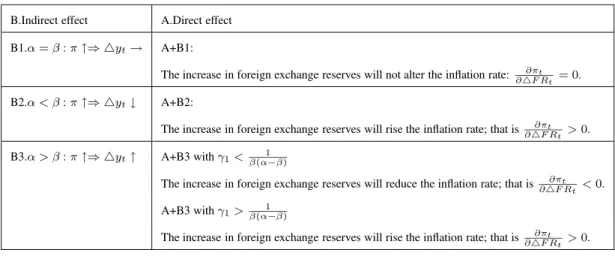
The summary of our conclusion is shown in Table 1.
Table 1 Summary of the theoretic conclusion B.Indirect effect A.Direct effect
B1.α = β : π ↑⇒ 4yt→ A+B1:
The increase in foreign exchange reserves will not alter the inflation rate: ∂πt ∂4F Rt = 0.
B2.α < β : π ↑⇒ 4yt↓ A+B2:
The increase in foreign exchange reserves will rise the inflation rate; that is ∂πt ∂4F Rt >0.
B3.α > β : π ↑⇒ 4yt↑ A+B3 with γ1<β(α−β)1
The increase in foreign exchange reserves will reduce the inflation rate; that is ∂πt ∂4F Rt <0.
A+B3 with γ1>β(α−β)1
The increase in foreign exchange reserves will rise the inflation rate; that is ∂πt ∂4F Rt >0.
3 Empirical Framework
To show how the intervention of the central bank influences the domestic economy, a simple regression model is set for the empirical study. We then describe the data and the econometric methodology utilized in our analysis.
3.1 The data
Our empirical study consists of five East Asian economies: Japan(JPN) and four “Tigers” (Hong Kong(HK), Korea(KOR), Singapore(SNG) and Taiwan(TWN)). The inflation rate is measured as the annual change in Consumer Price Index(CPI). The exchange rate is defined as the domestic currency price of a unit of the U.S. dollar. So the inflation rate of foreign country is the CPI inflation rate of U.S.. All the data are quarterly and span from 1981Q1 to 2003Q4, except from 1994Q1 to 2003Q4
for Hong Kong. The data for U.S., Japan, Hong Kong, Korea, Singapore are from
International Financial Statistics, IMF. For Taiwan, the data are from Financial Statistics Monthly Taiwan District, the central Bank of China.
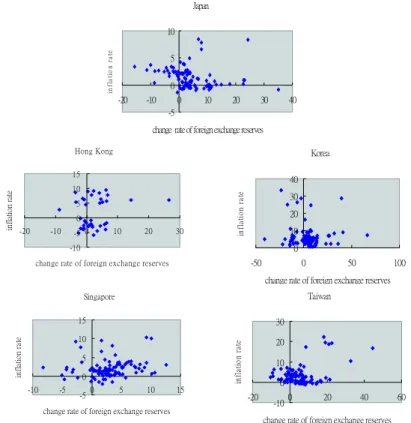
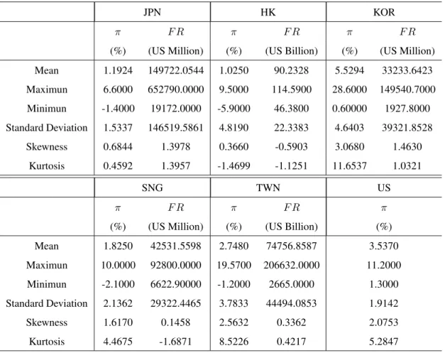
The descriptive statistics on inflation rate (π) and foreign exchange reserves (F R) are seen in Table 2. We also plot the scatter diagram with the change rate of foreign exchange reserves on the horizontal axis and the inflation rate on the vertical axis for each economy in Figure 1. The correlation coefficient between these two variables is -0.4323 for Japan, 0.2216 for Hong Kong, -0.0500 for Korea, 0.1525 for Singapore, and 0.3352 for Taiwan.
Table 2. Basic statistics
JPN HK KOR
π F R π F R π F R
(%) (US Million) (%) (US Billion) (%) (US Million) Mean 1.1924 149722.0544 1.0250 90.2328 5.5294 33233.6423 Maximun 6.6000 652790.0000 9.5000 114.5900 28.6000 149540.7000 Minimun -1.4000 19172.0000 -5.9000 46.3800 0.60000 1927.8000 Standard Deviation 1.5337 146519.5861 4.8190 22.3383 4.6403 39321.8528 Skewness 0.6844 1.3978 0.3660 -0.5903 3.0680 1.4630 Kurtosis 0.4592 1.3957 -1.4699 -1.1251 11.6537 1.0321 SNG TWN US π F R π F R π
(%) (US Million) (%) (US Billion) (%) Mean 1.8250 42531.5598 2.7480 74756.8587 3.5370 Maximun 10.0000 92800.0000 19.5700 206632.0000 11.2000 Minimun -2.1000 6622.90000 -1.2000 2665.0000 1.3000 Standard Deviation 2.1362 29322.4465 3.7833 44494.0853 1.9142 Skewness 1.6170 0.1458 2.5632 0.3362 2.0753 Kurtosis 4.4675 -1.6871 8.5226 0.4217 5.2847
3.2 Econometric Methodology
To study the relationship between inflation rate and the foreign exchange reserves. We could estimate equation (1), (2) and (3) to get those parameters α, β, k, γ1 and
γ2. However, the estimation for the parameters of objective function γ1and γ2needs
more complicated econometric method. This is an important issue and is beyond the scope of our study. Therefore we decide to estimate equation (6) directly instead of estimating equation (1), (2) and (3) separately.
We suggest a regression model motivated by equation (6) as the following form πt = β0+ β1Trendt+ β24F Rt+ β3πtf + et, (8)
where Trendt is time trend, et is the disturbance term. 4F Rt denotes the annual
change rate of foreign exchange reserves. The sign of estimated coefficient β2 can
tell us the relation between inflation rate and the foreign exchange reserves. Fur-thermore, comparing the differences of coefficient estimator β2 among these five
economies, we may have a rough understanding about the structure of each econ-omy.
The regression can be estimated for each economy respectively or as a system of separate equations for the individual economy. We assume the disturbances are in-dependent across equations when the regressions are estimated by the first method. However, the second method known as seeming unrelated regressions (SUR) is al-lowing the disturbances across equations to be freely correlated.
3.3 Results
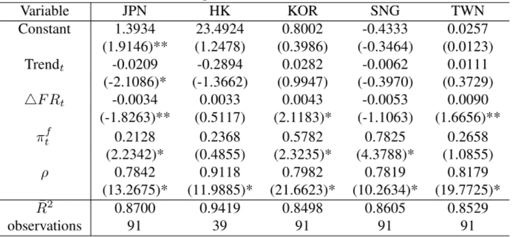
First, we estimate equation (8) for each economy respectively and this regression is named for Case 1 to differ from the seeming unrelated regressions. The regressions are estimated with a correction for serial correlation by Cochrane-Orcutt method. The empirical results are reported in Table 3. The inflation rate in Japan has sig-nificantly negative trend. And the trends in other four economies are not obvious. The inflation rate of U.S. is positively related to the domestic inflation rate in each economy.
The coefficient on 4F Rt is different among these five economies. For Japan,
on an average a 1% rise in foreign exchange reserves leads to a 0.0034% fall in inflation rate. However, on an average a 1% rise in foreign exchange reserves results in a 0.0043% rise in inflation rate of Korea and a 0.0090% rise in inflation rate of Taiwan. This relation is significant for Japan, Korea and Taiwan. Similarly, on an average a 1% rise in foreign exchange reserves invokes an inflation response of approximately 0.0033% for Hong Kong, -0.0053% for Singapore. In these two economies, nevertheless, this relation is insignificant.
Table 3. Case 1 : Estimated results of equation (8) in each economy respectively Dependent variable: πt Variable JPN HK KOR SNG TWN Constant 1.3934 23.4924 0.8002 -0.4333 0.0257 (1.9146)** (1.2478) (0.3986) (-0.3464) (0.0123) Trendt -0.0209 -0.2894 0.0282 -0.0062 0.0111 (-2.1086)* (-1.3662) (0.9947) (-0.3970) (0.3729) 4F Rt -0.0034 0.0033 0.0043 -0.0053 0.0090 (-1.8263)** (0.5117) (2.1183)* (-1.1063) (1.6656)** πft 0.2128 0.2368 0.5782 0.7825 0.2658 (2.2342)* (0.4855) (2.3235)* (4.3788)* (1.0855) ρ 0.7842 0.9118 0.7982 0.7819 0.8179 (13.2675)* (11.9885)* (21.6623)* (10.2634)* (19.7725)* ¯ R2 0.8700 0.9419 0.8498 0.8605 0.8529 observations 91 39 91 91 91
1.The regressions are estimated with a correction for serial correlation by Cochrane-Orcutt method.
2. The t-statistics are given in parentheses. 3. *(**) indicates significant at 5% (10%).
Equation (8) can also be estimated as a system of separate equations for the in-dividual economy. We use generalized least squares (GLS) to estimate this system. The standard errors are computed from heteroscedastic-consistent matrix developed by White (1980). Because the sample period for Hong Kong is not as long as other four economies, we estimate this system by two periods of analysis: Case 2 is from 1981Q1 to 2003Q4 for four economies excluding Hong Kong, and Case 3 is from 1994Q1 to 2003Q4 for all five economies. The results are presented in Table 4 and Table 5 respectively.
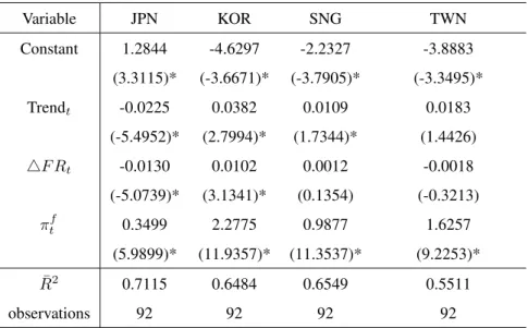
To simplify the analysis, we focus on the first point of our argument that is the relation between inflation and foreign exchange reserves. Table 4 shows that the sign of coefficient on 4F Rt is negative for Japan and is positive for Korea. Both
are significantly different from zero. This result of Case 2 is exactly the same in quality as Case 1. However, the coefficient on 4F Rt is not significant in Singapore
and Taiwan.
Finding of Table 5 indicates that the sign of coefficient on 4F Rtis significantly
positive for Korea and Taiwan which is similar to the result in Case 1. For Japan, Hong Kong and Korea, the coefficient is insignificant, nevertheless.
To sum up, the coefficient on 4F Rt is significantly positive for Korea in three
cases we estimate. And the value of the coefficient reveals that on an average a 1% rise in foreign exchange reserves invokes an inflation response of approximately 0.0043% to 0.0102%. The sign is significantly negative for Japan and the
signifi-cance is weak in Case 3. For those significant cases, an average a 1% rise in foreign exchange reserves leads to about 0.0034% to 0.0130% fall in inflation rate. For Taiwan, an average a 1% rise in foreign exchange reserves results in about 0.0090% to 0.0163% rise and this positive relation disappears in Case 2. And this relation is not evident in Hong Kong and Singapore.
Though the significance and magnitude of the coefficient on 4F Rt are not
ro-bust to the sample period or the estimation method we choose, we still have some rough findings from the empirical study in this section. The main conclusion is that the monetary surprise effect is strong in Japan. And the exchange rate effect may be powerful in Korea and Taiwan probably. These two effects are approximately equivalent in Hong Kong and Singapore.
The results could be interpreted by the structure of each economy. For the pe-riod 1986 to 2003, the average trade dependency ratio7is 16.51% for Japan, 55.91%
for Korea, 81.83% for Taiwan, 286.08% for Singapore, and 231.02% for Hong Kong. We argue that Japan is a large economy and the trade dependence is relatively smaller than other economies. We guess in Japan the impact of international trade on output may not be as strong as that of other factor such as the domestic monetary effect. However, Korea and Taiwan are both small open economies where the inter-national trade will play very important role in economic growth. Thus we suspect that in these two economies the exchange rate effect should dominate the domestic monetary surprise effect. Hong Kong and Singapore are like cities. Though the trade dependency ratios in these economies are large, the domestic monetary effect will influence the whole economy as well. By the empirical result, we conclude these two forces are approximately balanced in Hong Kong and Singapore.
Table 4. Case2: Estimated results of equation (8) by SUR: 1981Q1 to 2003Q4 Dependent variable: πt Variable JPN KOR SNG TWN Constant 1.2844 -4.6297 -2.2327 -3.8883 (3.3115)* (-3.6671)* (-3.7905)* (-3.3495)* Trendt -0.0225 0.0382 0.0109 0.0183 (-5.4952)* (2.7994)* (1.7344)* (1.4426) 4F Rt -0.0130 0.0102 0.0012 -0.0018 (-5.0739)* (3.1341)* (0.1354) (-0.3213) πtf 0.3499 2.2775 0.9877 1.6257 (5.9899)* (11.9357)* (11.3537)* (9.2253)* ¯ R2 0.7115 0.6484 0.6549 0.5511 observations 92 92 92 92
1. The t-statistics are given in parentheses. 2. *(**) indicates significant at 5% (10%).
Table 5. Case3: Estimated results of equation (8) by SUR: 1994Q1 2003Q4 Dependent variable: πt Variable JPN HK KOR SNG TWN Constant 3.9990 33.1612 11.5167 3.1571 10.2683 (4.2342)* (9.9101)* (5.0102)* (2.7601)* (9.1923)* Trendt -0.0406 -0.3900 -0.0846 -0.0557 -0.1328 (-4.1420)* (-11.1956)* (-3.5720)* (-4.6977)* (-10.7723)* 4F Rt -0.0065 0.0111 0.0091 0.0014 0.0163 (-1.4264) (0.8893) (2.3468)* (0.0176) (2.3391)* πtf -0.2973 -0.6723 -0.4543 0.8911 0.4826 (-1.7312)** (-1.1114) (-1.0908) (4.3555)* (2.3433)* ¯ R2 0.3545 0.7720 0.2773 0.5768 0.7769 observations 40 40 40 40 40
1. The t-statistics are given in parentheses. 2. *(**) indicates significant at 5% (10%).
4 Conclusions
Our study is an extension of the consistency model developed by Kydland and Prescott (1977). However, we consider the exchange rate stability as the policy-maker’s objectives additionally. Through the operations in the foreign exchange market by central bank, we are then able to analyze the relation between foreign exchange reserves and inflation rate. Our main conclusion is that when the foreign exchange reserves increases (or the domestic currency depreciates), the inflation will be rising while the exchange rate effect is stronger than monetary surprise ef-fect. And the inflation rate will be reduced when the monetary surprise effect is powerful if the weight placed on output stability is not large.
We use the data for five East Asian economies to make our argument more clear. The empirical result shows that the relation between the change in foreign exchange reserves and inflation rate is negative for Japan and is positive for Korea and Tai-wan. And this relation is insignificant for Hong Kong and Singapore. However, the significance is not robust to the sample period or the estimation method we utilize. The brief conclusion from our empirical study is that the monetary surprise effect is strong in Japan. And the exchange rate effect may be powerful in Korea and Tai-wan possibly. These two effects are approximately equivalent in Hong Kong and Singapore.
References
Alesina, A. and L. Summers (1993), ”Central Bank Independence and Macroeco-nomic Performance,” Journal of Money, Credit, and Banking, 25(2), 157-162. Barro, R. J. and D. Gordon (1983a), “A Positive Theory of Monetary Policy in a
Natural Rate Model,” Journal of Political Economy, 91(4), 589-610.
Barro, R. J. and D. Gordon (1983b), “Rules, Discretion and Reputation in a Model of Monetary Policy,” Journal of Monetary Economics, 12(1), 101-122.
Borjas, G. and V. Ramey (1995), “Foreign Competition, Market Power, and Wage Inequality,” Quarterly Journal of Economics, 110(4), 1075-1110.
of Inflation Explain Cross-country Differences in Inflations Dynamics?”
Jour-nal of Internationl Money and Finance, 23, 735-759.
Branson, W. and J. Love (1988), “United States Manufacturing and the Real Ex-change Rate,” In R. Marston, ed., Misalignment of ExEx-change Rates: Effects on
Trade and Industry, University of Chicago Press.
Burgess, S. and M. M. Knetter (1996), “An International Comparison of Employ-ment AdjustEmploy-ment to Exchange Rate Fluctuations,” NBER Working Paper 5861. Campa, J., and L. Goldberg. (1999), “Investment Pass-Through and Exchange Rates: A Cross-Country Comparison,” International Economic Review, 40:2, 287-314.
Cukierman, A. (1992), Central Bank Strategy, Credibility and Independence, MIT Press. Cambridge, MA.
Cukierman, A., P. Kalaitzidakis, L. H. Summers, and S. B. Webb (1993), “Central Bank Independence, Growth, Investment, and Real Rates,” Carnegie-Rochester
Conference Series On Public Policy, 39, 95-140.
Dominguez, K. M. and J. A. Frankel (1993), “Foreign Exchange Intervention: an Empirical Assessment,” In Frankel, J. A. (Ed), On Exchange Rate, MIT Press. Crambridge.
Eijffinger, S. and J. de Haan. (1996), The Political Economy of Central Bank
Inde-pendence, Special Papers in International Economics, No 79, Princeton
Univer-sity , Princeton, NJ.
Eijffinger, S. and E. Schaling (1993), “Central Bank Independence in Twelve In-dustrial Countries,” Banca Nazionale del Lavoro Quarterly Review, 184, 49-89. Fischer, A. M. and M. Zurlinden (1999), “Exchange Rate Effects of Central Bank Interventions: an Analysis of Transaction Prices,” Economic Journal, 109, 662-676.
Ghosh, A. R., J. D. Ostry, A. Gulde, and H. C. Wolf (1995), “Does the Nominal Exchange Rate Regime Matter?” IMF working Paper 95/121.
Giavazzi, F. and M. Pagano (1988), “The Advantage of Tying One’s Hands: EMS Discipline and Central Bank Independence,” European Economic Review, 32,
1055-1075.
Goldberg, L. and J. Tracy (1999), “Exchange Rates and Local Labor Markets,” NBER Working Paper 6985.
Gourinchas, P.-O. (1999), “Exchange Rates Do Matter: French Job Reallocation and Exchange Rate Turbulence, 1984-1992,” European Economic Review, 43, 1279-1316.
Kohli, R. (2003), “Real Exchange Rate Stabilisation and Managed Floating: Ex-change Rate Policy in India, 1993-2001,” Journal of Asian Economics, 14, 369-387.
Kydland, F. E., and E. C. Prescott (1977), “Rules Rather than Discretion : the In-consistency of Optimal Plans,” Journal of Political Economy, 85(3), 473-492. McCallum, B. T. (1989), Monetary Economics, New York: Macmillan.
McCallum, B. T. (1996), International Monetary Economics, New York: Oxford University Press.
Neely, C. J. (2000), “The Practice of Central Bank Intervention : Looking Under the Hood,” Central Banking 11, 24-37.
Obstfeld, M. (1996), “Models of Currency Crises with Self-fulfilling Features,”
Eu-ropean Economic Review, 40, 1037-1047.
Olson, M., Jr. (1996), “Big Bill Left on the Sidewalk: Why Some Nations Are Rich and Others Poor?” Journal of Economic Perspectives, 10(2), 3-24.
Payne, R. and P. Vitale (2001), “A Transaction Level Study of the Effects of Central Bank Intervention on Exchange Rates,” CEPR Discussion Paper 3085.
Persson, T. and G. Tabellini (1993), “Designing Institutions for Monetary Stability,”
Carnegie-Rochester Conference Series on Public Policy, 39, 53-84.
Pollard, P. S. (1993). “Central Bank Independence and Economic Performance,”
Federal Reserve Bank of St. Louis Review,, 75(4), 21-36.
Posen, A. (1995), “Declarations Are Not Enough: Financial Sector Sources of Central Bank Independence,” In B. Bernanke and J. Rotemberg (Ed), NBER
Revenga, A. (1992), “Exporting Jobs? The Impact of Import Competition on Em-ployment and Wages in U.S. Manufacturing,” Quarterly Journal of Economics, 107(1), 255-284.
Rogoff, K. (1985), “The Optimal Commitment to an Intermediate Monetary Tar-get,” Quarterly Journal of Economics, 100(4), 1169-1189.
Svensson, L. E. O. (1997), “Optimal Inflation Contracts, ’Conservative’ Central Banks, and Linear Inflation Contracts,” American Economic Review, 87(1), 98-114.
Vitale, P. (2003), “Foreign Exchange Intervention: How to Signal Policy Objectives and Stabilise the Economy,” Journal of Monetary Economics, 50, 841-870. Waller, C. J. and C. E. Walsh, (1996), “Central Bank Independence, Economic
Be-havior and Optimal Term Lengths,” American Economic Review, 86(5), 1139-1153.
Walsh, C. E. (1995), “Optimal Contracts for Central Bankers,” American Economic
Review, 85(1), 105-167.
White, H. J. (1980), “A Heteroskedasticity-Consistent Covariance Matrix Estimator and a Direct Test for Heteroskedasticity,” Econometrica, 48:4, 817-838.