Structural Cointegration Analysis of
Private and Public Investment
Rosemary Rossiter*
Department of Economics, Ohio University, U.S.A.
Abstract
A structural cointegration approach is used to investigate the relationship between public and private investment, based on dataseries which include software in the definitions of in-vestment. Empirical evidence for equipment suggests crowding out. However structures shows crowding in, supporting the infrastructure hypothesis.
Key words: structural cointegration approach; public investment JEL classification:C50; E22; E69
1. Introduction
Studies by Aschauer (1989a, 1989b, 1993) have rekindled interest in the effect of government provision of public investment on the private economy. Short-run Keynesian models which focus on the demand-side effects of government spending conclude that public investment crowds out some though not all private investment spending. However Aschauer, along with Buiter (1977), Munnell (1992), and others, also recognizes that public investment may complement private investment by en-hancing the productivity of existing resources (the infrastructure hypothesis).
A variety of empirical approaches have been used to estimate the impact of public capital stock on aggregate production technologies or private investment functions [Lynde and Richmond (1992), Erenburg (1993), Evans and Karras (1994), and Demetriades and Mamuneas (2000)]. However two persistent problems have been non-stationarity of variables and the quality of data for public and private in-vestment, at least for national accounts of the United States.
The first purpose of this paper is to use a structural cointegration approach to investigate the relationship between public and private investment. The structural cointegration approach of Pesaran and Pesaran (1997) and Pesaran and Smith (1998) encourages links between the new literature of cointegrating vector autoregressions and the more traditional literature of dynamic structural econometric modeling. Key
Received August 18, 2001, accepted October 29, 2001.
*Correspondence to: Department of Economics, Haning 237, Ohio University, Athens OH 45701, U.S.A.
aspects of this approach are the use of theory to identify multiple cointegration vec-tors and the treatment of stationary or non-stationary exogenous variables. The new literature also suggests the use of model selection criteria, accompanied by diagnos-tic tests, to specify short-run dynamics, determinisdiagnos-tic components, and cointegration rank and includes measuring the speed of convergence to equilibrium with persis-tence profiles.
A second goal of this paper is to highlight new data series for the U.S. economy which for the first time include spending for computer software in the definitions of public and private investment in equipment [Moulton, Parker, and Seskin (1999)]. The new series are the product of two recent comprehensive revisions which have brought the U.S. accounts into closer conformity with the national accounts of other countries by presenting newly-defined series for government consumption expendi-tures and government investment. For a discussion of several aspects of the revi-sions, see Rossiter (2000).
In the results presented below, the structural cointegration approach supports the conclusion that in the long-run public investment in equipment crowds out pri-vate investment. However, analysis of investment in structures suggests there is also support for the infrastructure hypothesis, with a convergence to equilibrium which takes several years.
2. Testing the Infrastructure Hypothesis
On the microeconomic level, new theories of investment under uncertainty have been developed based on the intuition of financial options [Hubbard (1994)]. However, on the aggregate level, the infrastructure hypothesis can be most appro-priately investigated by a modification of the traditional accelerator cash flow model of private investment.
The distinguishing feature of a traditional accelerator model based on an ad-justment cost approach is the assumption that investment depends on changes in output [Eisner and Strotz (1963)]. Empirical specifications commonly include a de-mand variable such as capacity utilization to capture other business cycles effects. Finally a profit or cash flow variable can be used because profits signal increased future output that increases the optimal path of future capital stock and lowers fi-nancing costs.
The traditional accelerator cash flow model can be modified to investigate linkages with public investment by including public investment as an explanatory variable. If higher public investment raises the rate of national capital accumulation, rational private sector agents will alter their investment plans in order to reestablish an optimal level of capital. Thus a modified accelerator cash flow equation may show that public investment crowds out private investment. However Aschauer suggests that there is a second link between public and private investment because public capital raises the return to private capital in private production technology. This second link implies that the stock of public capital crowds in private capital accumulation.
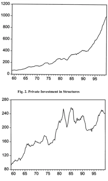
The empirical results below are obtained using fixed investment in equipment or structures, with chained (1996) dollar measures for the nonresidential component of the private sector and for defense, nondefense, and state and local government. Cashflow is corporate profits after taxes, adjusted for inventory valuation and a capital consumption allowance, and output is gross domestic product minus gross housing product. In the empirical work, all variables are measured as logarithms from 1954.1 to 1998.4. The structures and equipment components of public and pri-vate investment in chained (1996) dollars are shown in four figures.
Fig. 1. Private Investment in Equipment
Fig. 3. Public Investment in Equipment
Fig. 4 Public Investment in Structures
Fig. 4. Public Investment in Structures
3. Statistical Model
The modified accelerator cash flow model of investment may be appropriately modeled as a structural cointegrating vector autoregression where there are minimal restrictions on short-run dynamics and a long-run cointegration relationship is de-rived from the accelerator cash flow theory. An appropriate starting point for this approach is an error correction model as in Pesaran and Pesaran (1997) and Pesaran and Smith (1998):
n t w z z t a a y y t t p i i t iy t y y y t , 1 ,2, , 1 1 1 1 0 + −Π + Γ ∆ +Ψ + = K = ∆
∑
− = − − ε,
(1)where y is a (t my×1) vector of endogenous I(1) variables, x is a (t mx×1) vector of I(1) exogenous variables, zt =(yt′, xt′)′, w is a (t q×1) vector of ex-ogenous I(0) variables excluding intercepts and trends, and t is a time trend. The symbol ∆ is the difference operator, and all other symbols such as a0y or
y
Π represent coefficients. The model assumes that there is feedback from ∆y to
x
∆ but no feedback in levels, so that x is given as t
t t x p i i t xi x t a z w v x = + Γ ∆ +Ψ + ∆
∑
− = − 1 1 0,
(2)and the disturbances ε and t v are t iid(0,Σ) with Σ a symmetric posi-tive-definite matrix, and ε and t v are distributed independently of t w . Theory t
suggests that private and public investment and cashflow can be considered en-dogenous variables while the utilization rate and change in output are exogenous. If
t
y is cointegrated, the matrix Π will have reduced rank with r cointegration vec-tors, one or more of which might include private and public investment.
In order to uniquely identify multiple vectors, it would be necessary to impose at least r restrictions on each of the vectors but if r=1, normalization produces exact identification.
If there are linear trends in an unrestricted vector autoregression, cointegration will mean quadratic trends in levels of the variables unless trends are restricted to the cointegrating vectors. If intercepts are restricted to the cointegrating vectors, then
t
y will contain a linear deterministic trend. Thus it is important that equation (1)
explicitly models intercepts and trends. If the variables y and t x have determi-t
nistic trends, the most appropriate action may be to restrict the trend coefficients. Otherwise it would be appropriate to restrict intercepts to the cointegrating vectors.
Lastly, conventional cointegration analysis has used model selection criteria to choose leg length in the error correction model while intercepts and deterministic trends are chosen a priori. Johansen maximum eigenvalue and trace tests are then used to determine the number of cointegration vectors. Mills (1998), Pesaran and Smith (1998), and Phillips (1998) have suggested using a Schwarz or Phillips crite-rion to select the lag length simultaneously with the number of cointegration vectors and treatment of intercepts and trends. However because many of these tests have low power, the specification of (1) must be confirmed by diagnostic checks for serial correlation. The empirical work presented below uses the Schwarz criterion to spec-ify a statistical model, followed by standard diagnostic tests. All calculations are performed using Microfit 4.0 (Camfit Data Ltd, 1997).
4. Empirical Results
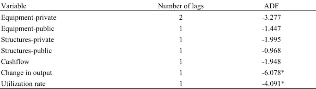
Augmented Dickey-Fuller test statistics were found for each variable, with the number of lags determined by Schwarz criteria. The results presented in Table 1 show that only the utilization rate and the change in output are stationary. Thus in what follows we proceed as if equation (1) contains stationary exogenous variables only.
Table 1. Augmented Dickey-Fuller Unit Root Tests
Variable Number of lags ADF
Equipment-private 2 -3.277 Equipment-public 1 -1.447 Structures-private 1 -1.995 Structures-public 1 -0.968 Cashflow 1 -1.948 Change in output 1 -6.078* Utilization rate 1 -4.091*
The Schwarz Bayesian criterion was used to select number of lags. Critical values at the .05 level for the ADF test are -2.880 for private and public structures, change in output and the utilization rate and -3.439 for all other variables.
As a first step in specifying the model, the Schwarz criterion was calculated for lags ranging from 1 to 6 for all possible cointegration vectors for models with either restricted intercepts and no trends or unrestricted intercepts and restricted trends. Using a model selection criterion is advisable given the well-known problems asso-ciated with determining the number of cointegration vectors. Specifically, the Johansen trace and maximum eigenvalue tests for cointegration rank perform unre-liably in finite samples and often lead to different conclusions. Moreover, the selec-tion of rank is sensitive to the order of the vector-autoregressive component of the model as well as to the treatment of intercepts and trends.
Empirical results for investment in equipment confirm the importance of re-stricting intercepts or trends when investigating whether a model is cointegrated. In the case of restricted intercepts, the Schwarz criterion consistently suggests a lack of cointegration, with the highest values of the criterion occurring at r=0 for lags 1 through 6. (Tabular results for equipment and structures are available upon request.) However in the case of restricted trends, the criterion suggests one cointegration vector at all lags. The maximum value of the criterion suggests a specification of restricted trends, one lag and one cointegration vector. Given that the data itself ex-hibits strong trends, these choices seem reasonable and are used below. However as additional checks of this specification we also present below the Johansen cointegra-tion test statistics and diagnostic tests for serial correlacointegra-tion in the error-correccointegra-tion equations.
For investment in structures, the maximum value of the criterion occurs at 0
=
r for lags 2 through 6 for both restricted intercepts and restricted trends. How-ever at a lag length of one, the criterion suggests r=1 for the case of restricted intercepts or r=2 for restricted trends. The maximum value of the criterion occurs
with restricted intercepts, and visual inspection of the data suggests that this is a reasonable choice. Hence a lag length of one is used for structures as well as equip-ment, with additional tests below to confirm this specification.
Table 2 presents the Johansen maximum eigenvalue and trace tests to deter-mine the number of cointegration vectors for the specifications suggested by the selection criteria. These test statistics strongly support the presence of one cointega-tion vector for equipment as well as structures. Hence these tests are in agreement with the specification selected using the Schwarz criterion.
Table 2. Johansen Cointegration Test Statistics Equipment
Maximum Eigenvalue Statistic Trace Statistic
0 : 0 r= H 47.27 64.91 1 : 0 r≤ H 10.85 17.64 2 : 0 r≤ H 6.78 6.78 Structures Maximum Eigenvalue Statistic Trace Statistic
0 : 0 r= H 42.51 53.64 1 : 0 r≤ H 6.43 11.12 2 : 0 r≤ H 4.69 4.69
For equipment, critical values at the .05 level are 25.42, 19.22, and 12.39 for the maximum eigenvalue test and 42.34, 25.77, and 12.39 for the trace test. For structures, critical values at the .05 level are 25.42, 19.22, and 12.39 for the maximum eigenvalue test and 42.34, 25.77, and 12.39 for the trace test.
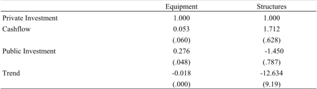
Table 3. Normalized Cointegration Vectors
Equipment Structures Private Investment 1.000 1.000 Cashflow 0.053 (.060) 1.712 (.628) Public Investment 0.276 (.048) -1.450 (.787) Trend -0.018 (.000) -12.634 (9.19) Numbers in parentheses are standard errors.
We normalize on private investment and test the long-run effect of public on private investment. Maximum likelihood estimates of the cointegration coefficients and standard errors are presented in Table 3. In each case, the structural interpreta-tion of the long-run cointegrainterpreta-tion equainterpreta-tion implies that private investment would be the left-hand-side variable. Thus the coefficient on public investment indicates a negative relationship between public investment and private investment in equip-ment, that is to say, support for the hypothesis that public investment in equipment crowds out private investment. The Chi-square test of the statistical significance of the coefficient is 23.42 (p=.000), confirming that public investment should be
in-cluded in the long-run equation for private investment. The coefficient on cashflow is not statistically significant and there is a statistically significant positive trend.
In contrast, the coefficient on public investment in the structures equation is negative, suggesting public investment crowds in private investment. The Chi-square test of the coefficient is 3.12 (p=.077). Thus this long-run equation provides weak evidence that public investment in structures crowds in private in-vestment. However the size of the coefficient on public investment is unexpectedly large, as is the negative coefficient on cashflow, so that this equation is not entirely satisfactory. For both structures and equipment, error correction terms were statisti-cally significant in all equations except for public investment, and there was evi-dence of two-way feedback. Diagnostic statistics for equipment are satisfactory while in the case of structures there is evidence of heteroscedasticity and the adjust-ment weight in the private investadjust-ment equation has an unexpected positive sign.
Traditionally the last step in investigating a cointegration model is an impulse response analysis [Lutkepohl and Reimers (1992)]. Koop et al. (1996) have devel-oped a generalized impulse response function which does not require orthogonaliza-tion of shocks and is invariant to the ordering of variables. An alternative charac-terization of the effect of a system-wide shock is a persistence profile, defined as the scaled difference between the conditional variances of the n-step and (n-1)-step ahead forecasts. A scaled persistence profile will have a value of one on impact but will tend to zero if a relationship is cointegrated (even though the shock will have a permanent effect on the individual variables). In effect, the persistence profile is a test of cointegration which also illustrates the speed with which a relationship re-turns to equilibrium.
Persistence profiles for equipment and structures (available upon request) con-firm the evidence presented above, with a rapid convergence to equilibrium, rea-sonable for a relationship where crowding out is the result of financial constraints. However the persistence profile for structures suggests that the effect of a sys-tem-wide shock persists for many years, supporting the hypothesis that public in-vestment enhances private inin-vestment and productivity. However the coefficients of the cointegration vector and incorrect signs of the adjustment coefficients suggest caution in interpreting the structures model overall.
5. Conclusions
This paper uses a structural cointegration approach to test hypotheses of crowding out and crowding in. Empirical results suggest that public investment in equipment crowds out private investment, while public investment in structures has a weak crowding in effect.
References
Aschauer, D., (1989a), “Is Public Expenditure Productive?” Journal of Monetary
Economics, 23(1), 177-200.
Aschauer, D., (1989b), “Does Public Capital Crowd Out Private Capital?” Journal
of Monetary Economics, 24(2), 171-188.
Aschauer, D., (1993), “Genuine Economic Returns to Infrastructure Investment,”
Policy Studies Journal, 21(1), 380-390.
Buiter, W., (1977), “ Crowding Out and the Effectiveness of Fiscal Policy,” Journal
of Public Economics, 7(1), 309-328.
Demetriades, P. and T. Mamuneas, (2000), “Intertemporal Output and Employment Effects of Public Infrastructure Capital: Evidence from 12 OECD Economies,”
The Economic Journal, 110, 687-712.
Eisner, R. and R. Strotz., (1963), “Determinants of Business Investment,” Impacts of
Monetary Policy, Prentice-Hall.
Erenburg, S., (1993), “The Real Effects of Public Investment on Private Invest-ment,” Applied Economics, 25(6), 831-837.
Evans, P. and G. Karras, (1994), “Is Government Capital Productive? Evidence from a Panel of Seven Countries,” Journal of Macroeconomics, 16(2), 271-279. Hubbard, R. G., (1994), “Investment under Uncertainty: Keeping One’s Options
Open,” Journal of Economic Literature, 32(4), 1816-1831.
Koop, G., M. H. Pesaran, and S. Potter, (1996), “Impulse Response Analysis in Nonlinear Multivariate Models,” Journal of Econometrics, 74(1), 119-147. Lutkepohl, H. and H. E. Reimers, (1992), “Impulse Response Analysis of
Cointegrated Systems,” Journal of Economic Dynamics and Control, 16(1), 53-78.
Lynde, C. and J. Richmond, (1992), “The Role of Public Capital in Production,” The
Review of Economics and Statistics, 74(2), 37-44.
Mills, T., (1998), “Recent Developments in Modeling Nonstationary Vector Autore- gressions,” Journal of Economic Surveys, 12(3), 279-312.
Moulton, B., R. Parker, and E. Seskin, (1999), “A Preview of the 1999 Comprehen-sive Revision of the National Income and Product Accounts: Definitional and Classificational Changes,” Survey of Current Business August, 7-20.
Munnell, A., (1992), “Policy Watch: Infrastructure Investment and Economic Growth,” The Journal of Economic Perspectives, 5(3), 189-198.
Pesaran, M. H. and B. Pesaran, (1997), Working with Microfit 4.0. Camfit Data
Lim-ited, Cambridge, England.
Pesaran, M. H. and R. Smith, (1998), “Structural Analysis of Cointegrating VARS,”
Journal of Economic Surveys, 12(5), 471-505.
Phillips, P. C. B., (1998), “Impulse Response and Forecast Error Variance Asymp-totics in Nonstationary VARS,” Journal of Econometrics, 83(1), 21-56. Rossiter, R., (2000), “Fisher Ideal Indexes in the National Income and Product Ac