背景風險下之最適投資組合：建構不完全市場下之隨機控制模型(II)

行政院國家科學委員會專題研究計畫 成果報告

背景風險下之最適投資組合：建構不完全市場下之隨機控制

模型(2/2)

計畫類別： 個別型計畫 計畫編號： NSC93-2416-H-004-004- 執行期間： 93 年 08 月 01 日至 94 年 07 月 31 日 執行單位： 國立政治大學風險管理與保險學系 計畫主持人： 張士傑 報告類型： 完整報告 處理方式： 本計畫涉及專利或其他智慧財產權，1 年後可公開查詢

中 華 民 國 94 年 10 月 31 日

行政院國家科學委員會補助專題研究計畫成果報告

背景風險下之最適投資組合：

建構不完全市場下之隨機控制模型

Optimal Investment Strategy under Background Risks:

Stochastic Control Models under Incomplete Market

計畫類別：個別型計畫

計畫編號：NSC 93－2416－H－004－004－

執行期間：2004 年 8 月 1 日至 2005 年 7 月 31 日

計畫主持人：張士傑

成果報告類型：完整報告

執行單位：國立政治大學風險管理與保險學系

中 華 民 國 94 年 10 月 31 日

Abstract

In this study, we investigate the portfolio selection problem in order to hedge the background risks, i.e., labor income and inflation rates in the defied contribution (DC) pension schemes under incomplete market. First, we extend the previous work of Battocchio and Menoncin (2004) that allowed the state variables (i.e., the risks from the financial market) and a set of stochastic processes to describe the inflation, labor income and expense uncertainties. A five-fund separation theorem is derived to characterize the optimal investment strategy for DC pension plans to hedge the labor income and the inflation risks. Second, by solving the Hamiltonian equation in the three-asset framework, we show that the optimal portfolio consists of five components: the myopic market portfolio, the hedge portfolio for the state variables, the hedge portfolio for the inflation risk, the hedge portfolio for the labor income uncertainty and the riskless asset. Then we explicitly solve the optimal portfolio problem. Finally, the numerical results indicate that the inflation hedge portfolio comprises the overwhelming proportion of stock holdings in the optimal portfolios. In addition, the inflation hedge portfolio and the state variable hedge portfolio constitute the overwhelming proportions of bond holdings.

Keywords: defined contribution; salary uncertainty; inflation; stochastic control; dynamic programming. 摘要 本文探討不完備市場下規避背景風險之最適投資組合，以確定提撥退休金計畫為對象，探 討基金經理人如何決定最適資產策略規避薪資所得及通貨膨脹之不確定風險，求得期末財 富效用期望值極大化。本研究首先擴展Battocchio與 Menoncin (2004)所建構之資產模型， 我們不僅探討來自市場之風險，同時考量薪資所得、 通貨膨脹與費用率之不確定性，研究 其對最適資產配置行為的影響，建構隨機控制模型，以動態規劃方法求解Hamiltonian方程 式，研究結果顯示，我們可利用五項共同基金分離定理來描述投資人之最適投資決策：短 期市場基金、狀態變數避險基金、薪資所得避險基金、通貨膨脹避險基金與現金部位。數 值結果顯示，股票持有部位中通貨膨脹避險基金佔有最大的成份，債券持有部位中通貨膨 脹避險基金與狀態變數避險基金佔有最大的成份。 關鍵字：確定提撥、薪資所得、通貨膨脹、隨機控制、動態規劃

1. INTRODUCTION

Although the defined contribution (hereafter DC) pension plans have been the primary engine of growth in the U.S. private pension market over the last two decades (see Lachance et al., 2003), the pension systems in most of Asian countries have traditionally been more tied to defined benefit (hereafter DB) pension plans. The benefits in DB plans are fixed in advance and the plan sponsor adjusts the contributions annually, whereas the benefits in DC plans are determined by the performance of the invested portfolio and the contributions are fixed. But recently the legislatures in many Asian countries have introduced DC pension schemes into their pension system. To do so, they either reform their pension to DC schemes or plan to restructure their retirement program to a mixture of DC and DB pension schemes. A DC plan offers participants not only the flexibility and the portability but also the investment portfolio choice, all of which can improve an employer’s ability to attract and retain workers. But the investment risk that had been assumed by the plan sponsor under the DB promise is transferred to the worker in a DC plan (Bodie, 1990).

Recently, some states in the U.S. have introduced a guarantee mechanism to help protect DC plan participants. One such guarantee takes the form of an option permitting DC plan participants to buy back their DB benefit for a price (see Lachance et al., 2003; Milevsky and Promislow, 2004). Lachance et al. (2003) found that if employees were to exercise the buy-back option optimally, the market value of this option could represent up to 100 percent of the DC contributions over their work life. Thus the potential costs involved with the provision of such a guarantee are easily misunderstood and can be quite large. In this study, not only is a theoretical frame-work developed to analyze the optimal portfolio strategy but we also illustrate how the portfolio characteristics influence the behaviors of the wealth accumulation. Asset allocation is a decision-making process in which the investment funds of an individual or a group of individuals are allocated to investment categories rather than to individual assets. Studies by Brinson, et al. (1986, 1991) have shown convincingly that allocation of investment funds to asset categories is far more important than the selection of individual securities within each asset category.

Since a major part of the wealth of the plan participant comes from the labor income and may suffer from the inflation risk due to the long time before his retirement, three issues listed in the following are considered and investigated in detail.

1. How can the dynamic hedge demands for future inflation and labor income uncertainties be incorporated in making the long-term financial planning for retirement?

2. How can the incentive fees or the floor protections provided in the fund management be reasonably controlled through the capital market, based on the mutual fund separation theorem?

3. How can the risks and rewards from the financial market be reasonably considered with different risk factors, investment time horizons and attitudes toward risks?

It is the investment performance of pension funds that has become a crucial theme in more recent years, especially due to the aging society worldwide. Pension contributions can be regarded as a form of mandatory savings for the plan participants before their retirement. According to the Labor Worker Standard Law enacted by Taiwan government in 1984, an

employer is required to contribute 2% to 15% of each employee’s pensionable payroll to a government-managed trust fund with minimum returns guaranteed by the government. The mandatory pension plan is a defined benefit scheme since the participant’s retirement benefits are calculated according to the length of employed time and the final salary upon retirement. With over seven million employees, the labor worker retirement system is one of the major pension plans in Taiwan. Although the pension plan has minimum guaranteed returns from the government, the plan is subject to insolvency risk because the insufficient contributions coupled with low investment returns may not be able to match the benefit payments.

After lengthy debates over several decades, the Legislation Yuan in Taiwan finally reformed its Labor Standard Law in June 2004. The legislature has adopted a new system that provides two kinds of retirement options to the labor workers through the personal retirement account and the annuity insurance program. This new system will be enacted in July 2005. Under article 6, employers shall contribute on a monthly basis to the Labor Pension Fund by contributing into the individual pension fund accounts at the Bureau of Labor Insurance for those employees who are subject to this Act. Under the personal retirement account, the retirement provisions for the new labor workers belong to the defined contribution schemes, and the rate of contribution by an employer to the Labor Pension Fund per month shall not be less than 6% of the employee’s monthly wages. An employee may voluntarily contribute per month, up to 6% of his/her monthly wages to his/her pension fund account. The full amount of the voluntary pension contribution made by an employee may be deducted from the employee’s taxable income in the year concerned. Under article 24, an employee who is 60 years old or above and whose seniority is more than 15 years, is entitled to monthly pension payments. An employee whose seniority is less than 15 years shall be entitled to a lump sum pension payment.

The investment performance of the pension fund is guaranteed by the government and in accordance with this Act shall not be less than that of the interest paid for a two-year term time deposit by local banks. In the event of any deficiency, the Treasury shall make up the shortfall. The labor workers can also select the annuity insurance program run by the private insurance companies if the company has more than two hundreds employees and half of the employees agree to this arrangement. The labor workers are eligible to draw their pension at the age of sixty. In addition, this new system also provides the option for active workers to choose between the old system and the new one.

The change from the DB plans to the DC plans appears to be significant for plan participants, since the accumulation process of fund wealth is totally different from the previous systems. In the new DC scheme, the investment risk that was previously borne by the sponsors in DB plans has now devolved to the plan participants. In the DC pension plan, the fund manager plays a crucial role in providing the retirement benefits for the plan participants against the cost of living adjustment (COLA) since the final wealth at his retirement date depends on the fund performance. Therefore, a comprehensive study is required to clarify how the fund manager handles the pension assets to achieve the required performance under this new pension system.

A DB pension plan is a pension scheme where the benefits are defined in advance by the sponsor. Contributions are set and subsequently adjusted so as to ensure that the scheme remains in balance. Conversely, a DC pension plan is a pension scheme where only contributions are fixed and benefits therefore depend solely on the return of the assets. Thus, DC plans allow the contributors to trace the value of their retirement accounts. The only aspect that a plan participant can determine is to make reasonable assumptions on the replacement ratio, i.e. the percentage of her income which will be replaced by the pension. Currently, most of the proposed pension plans are based on DC schemes involving a considerable transfer of risks to employees. As we have already highlighted, the employee’s contributions are determined in advance, while the final retirement account depends on the administrative expenses and investment performance of the fund managers. Consequently, it is an efficient financial management that is essential to gain contributor’s trust.

1.2. The asset allocation problem

It is to invest the accumulated wealth to maximize the expected utility of the terminal fund wealth that the goal of the fund manager is. Most conventional pension management is constructed under one-period and constant interest rate assumptions, and uses the Markowitz (1952) approach, i.e. mean-variance method. Sharpe (1991) describes the mean-variance approach as a highly parsimonious characterization of investor goals, employing a myopic view and focusing on only two aspects of the probability distribution of possible returns over that period. The main drawback in the method which discussed in Sharpe (1991) is that the aggregation of single-period optimal decisions across periods might not be optimal for multiple periods as a whole. Similarly, the pension fund holders are usually long-term investors, generally from 20 to 40 years, the assumption of constant interest rates is not suitable for our purpose. Thus, pension plan management should be considered within multi-period framework. Methods of optimal control solve the long-term financial planning problems through global optimization across periods instead of local optimization within a period.

1.3. The developments of the multi-period problems

The control theory has been developed in engineering fields since the 1930s and the applications to economics emerged in 1950s. Samuelson (1969), Merton (1969, 1970, 1990), Brennan and Schwartz (1982), Karatzas et al. (1986), Karatzas and Shreve (1991), Duffie (1996), Kim and Omberg (1996), Brennan, Schwartz and Lagnado (1997), Boyle and Yang (1997), Brennan and Schwartz (1998), Sorensen (1999), Wachter (2002), and Campbell and Vicerira (1999, 2001) studied the optimal consumption and investment problems under different setting using the control theory.

The application of control theory to pension plan management began with O’Brien (1986, 1987). Subsequent papers along this line include Haberman and Sung (1994), Runggaldier (1998), Schäl (1998), Chang (1999, 2002), Chang et al. (2003) and related works. Cairn (2000) further introduces the asset allocation into the controlled process, studying the optimal investment strategies as well as optimal funding policies to minimize certain quadratic loss functions.

0 10000 20000 30000 40000 50000 60000 70000 80000 1988 1990 1992 1994 1996 1998 2000 2002 2004 year NTD

Josa-Fombellidal and Rincón-Zapatero (2001) minimize the contribution rate risk and the solvency risk with n risky assets and a risk-free security in the presence of short selling constraints. Chang et al. (2002) study the dynamic funding policy and investment strategy for the defined benefit pension schemes. They formulate the optimal decisions of pension plans as a stochastic control problem and solve the problem through dynamics programming. Chang et al. (2003) show that failing to recognize the under-funding risk and the over-contribution risk will lead to a significant difference in optimal funding schedule. Not merely the weighting factors but also the returns of investment play critical roles in obtaining the optimal strategy.

1.4. Background risks

Since the background risks proposed in Menoncin (2002) are not fully investigated in the previous pension studies, in addition to the state variables (i.e., the risks from the financial market), we consider a set of stochastic processes to describe the inflation and labor income uncertainties, called the background variables in this study. These factors significantly affect the growth of investor wealth and by means of incorporating these variables into the models we are capable of considering several crucial factors for financial planning.

First, it is the uncertainty of labor income that we consider since this has a profound effect on the plan contributions. According to Campbell and Viceira (2002), the investors own tradable financial assets as part of their total wealth portfolio, but they also own a valuable asset that is not readily tradable. This asset is their human wealth, the expected discounted value of their future labor income. Figure 1 shows that the personal average wages have changed every year from 1988 to 2004 in Finance and Insurance industries in Taiwan. Imrohoroglu, Imrohoroglu and Joines (1995) investigate the role of social security in a general equilibrium setting with salary uncertainty but non-stochastic rates of return and no annuities. Huang, Imrohoroglu and Sargent (1997) focus on the intergenerational impact of various social security systems on transition paths. They allow for stochastic salary uncertainty but there is no uncertainty on rates of return. Campbell, Cocco, Gomes and Maenhout (2001) consider the long-run pattern of lifetime savings and portfolio allocation in the presence of income and rate of return uncertainty and with various pension arrangements. Under no circumstances do they consider the impact of varying degrees of imperfection in annuity markets. On the contrary, they do consider fixed costs of entering the equity market. Since we consider the DC plan in which employees have to contribute a fixed rate of their income to their personal accounts. These can be regarded as personal pensions. Personal pensions mean that labor income risk from working years, which will have an impact on the contributions to a personal pension fund, has lasting effects upon pension income.

Figure. 1 Personal Average Salary in Finance and Insurance Industries in Taiwan (Data from Directorate General of Budget, Accounting and Statistics, Executive Yuan, R.O.C. on 9/28/2005.

http://win.dgbas.gov.tw/dgbas04/bc5/earning/ht4561.asp)

Campbell and Viceira (2002) discuss the effects due to the labor income risk. First, the existence of other income prospects tends to substitute for bonds in the investor portfolio. Hence a relatively young investor with extensive future earnings prospects will tend to have a higher proportion of stocks than an investor at a later stage of his working life. However, this effect is reduced if the income prospects are uncertain. In line with the literature on background risk, in effect the investor becomes more risk-averse to the market risks and, hence, buys less stock. Viceira (2001) optimizes the inter-temporal investment-consumption policy of an investor who has uncertain salary. In his model, labor income follows a geometric process and any savings out of labor income are invested in the portfolio. The single risky asset also follows a possibly correlated geometric process. Viceira finds that the ratio of portfolio wealth to labor income is stationary, and using a log-linear approximation he derives an optimal portfolio policy which has a constant stock proportion. Moreover, he also finds that when salary risk is independent of the asset return risk, employed investors hold a larger fraction of their savings in the risky asset than retired investors. Koo (1998) and Heaton and Lucas (1997) also derive optimal consumption and portfolio policies with stochastic wage. Koo uses a continuous time model and shows that the optimal level of risk taking is lower in the presence of an uninsurable labor income risk. Heaton and Lucas, in an infinite horizon model, do not find any significant effect of labor income risk on portfolio composition.

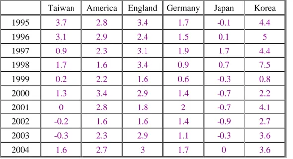
Second, it is the inflation risk that we take into account. Actually, when a long period of time is considered, this risk becomes significant. In Figure 2, we draw the Consumption Price Index (CPI) from 1995 to 2004 of the major countries worldwide. It can be seen that apart from Japan, all countries increase every year. The CPI data in Taiwan is selected and is shown in Figure 3, which shows that the CPI has fluctuated every year, so the inflation risk exists. Since the pension fund is a long-term plan, the managers should consider this inflation risk and determine the optimal strategy to resist the inflation uncertainties. Modigliani and Cohn (1979), Madsen (2002) and Ritter and Warr (2002) have shown that stock market investors suffer from inflation illusion. Menoncin (2002) considers both the salary uncertainty and also the inflation risk to analyze the portfolio problem of an investor maximizing the expected exponential utility of his terminal real wealth. In his model, the investor must cope with both a set of stochastic investment opportunities and a set of background risks. If the market is complete this model can find an exact solution. If the market is incomplete, they suggest an approximated general solution. Contrary to other exact solutions obtained in the literature, all their results are obtained considering a stochastic inflation risk and without specifying any particular functional form for the stochastic variables involved in the problem.

-2 0 2 4 6 8 1995 1996 1997 1998 1999 2000 2001 2002 2003 2004 year % Taiwan America England Germany Japan Korea -0.5 0 0.5 1 1.5 2 2.5 3 3.5 4 1995 1996 1997 1998 1999 2000 2001 2002 2003 2004 year %

Figure. 2 Consumption Price Index per year (Data from Directorate General of Budget, Accounting and Statistics, Executive Yuan, R.O.C. on 9/28/2005

http://www.dgbas.gov.tw/ct.asp?xItem=1633&ctNode=2252)

Figure. 3 Consumption Price Index in Taiwan (Data from Directorate General of Budget, Accounting and Statistics, Executive Yuan, R.O.C. on 9/28/2005 http://www.dgbas.gov.tw/ct.asp?xItem=1633&ctNode=2252)

1.5. The main approach in this article

In this article, we employ the dynamic programming approach presented in Battocchio and Menoncin (2004), in analyzing the optimal portfolio problem for a DC pension fund with labor income risk and inflation risk. We note that in Battocchio and Menoncin (2004), the constraint that the sum of the total invested assets should equal the fund wealth is not clearly verified. At the same time, since the fund performance is also significantly related to the fund management fee and the incentive bonus. Hence a detailed constraint for the assets and the management expenses are incorporated into our framework. The proposed model is summarized as follows.

1. The interest rates vary in the multi-period setting, so the stochastic model proposed in Vasicek (1977) is employed to describe its dynamics.

2. The financial market consists of three assets: a riskless asset (cash), stock index and bond fund, which can be bought and sold without incurring any transaction costs or restriction on short sales.

incomes and the uncertainties of the consumption price index.

4. The management incentives for the fund manager that the pension board must consider are incorporated in evaluating the financial decisions.

In order to fully characterize the characteristic of the DC pension plans, we consider a plan participant who, at each period, contributes a constant proportion of his/her salary income to a personal pension account. At the date of retirement, the accumulated pension fund will be converted into a life annuity.

Similar models have been recently presented by Blake et al. (2000), Boulier et al. (2001) and Deelstra et al. (2003). Especially, Blake et al. (2000) assume a stochastic process for salary including a non-hedgable risk component and focus on the replacement ratio as the central measure for determining the pension flow. Boulier et al. (2001) assume a deterministic process for salary and consider a guarantee on the benefits. Accordingly, they strongly support the real need for a downside protection of contributors who are more directly exposed to the financial risk borne by the pension fund. Also Deelstra et al. (2003) allow for a minimum guarantee in order to minimize the randomness of the retirement account; although they describe the contribution flow through a non-negative, progressive measurable and square-integrable process. A recent model for a DC pension scheme in discrete time is proposed by Haberman and Vigna (2001). In particular, they study both the investment risk, that is the risk of incurring a poor investment performance during the accumulation phase of the fund, and the annuity risk, that is the risk of purchasing an annuity at retirement in a particular recessionary economic scenario involving a low conversion rate.

It is dynamic programming that the methodological approach employed in solving the optimal asset allocation problem is. Alternative approaches (see for example Deelstra et al. (2003); Lioui and Poncet (2001)) are based on the Cox-Huang (1991) methodology (the so-called martingale approach), where the resulting partial differential equation is often simpler to solve than the Hamilton-Jacobi-Bellman equation from the dynamic programming. In this article, closed form solutions are constructed to understand the dynamic hedging demands through mutual fund separation theorem originally proposed in Merton (1971) for cases where different risk factors from the financial market, inflation and labor income are involved in the pension economy. An important result called five-fund separation is constructed, which means that investment choices are reduced to the allocation of assets between five specific investment funds (portfolio). Finally, the numerical simulations are presented to investigate the dynamics behavior of optimal portfolio strategy through several separated components.

The work is organized as follows. In Section 2, we introduce the general framework and reveal the financial market structure, the dynamics processes describing the behavior of asset values, the background risks of salary risk and inflation risk, and the fund’s wealth. In Section 3, not just do we present the stochastic optimal control problem but we also use the dynamic programming algorithm to compute the problem and derive an explicit solution. In Section 4, we present a numerical simulation. Finally, Section 5 concludes and summarizes the paper.

In this section, we focus on the financial model for DC pension plan that is fully investigated in this paper. First, the financial market is introduced and the stochastic processes are employed to characterize the dynamics of the interest rate and asset prices. Then the stochastic processes are presented to describe the behavior of two background risks: labor incomes and inflation rates. Finally, the accumulated nominal fund wealth and real wealth processes are derived.

2.1. Financial Market

The financial market is assumed to be arbitrage-free, complete and continuously open over the fixed time interval [ T , where 0, ] T >0 denotes the retirement time of a representative shareholder. Randomness is described by two standard and independent Wiener processes Wr(t) and )Wm(t , with t∈[ T0, ], and defined on a complete probability space(Ω,F,P). Here, P is the real world probability, and F ={F(t)}_t∈[0,T] is the filtration which represents the information structure assumed to be generated by Brownian motion and satisfying the usual conditions.

) (t

Wm is a standard Wiener process independent of Wr(t) capturing the asset risk other than the interest rate risk. The independence hypothesis on Wr(t) and Wm(t) implies no loss of generality since we can always shift from uncorrelated to correlated Wiener processes (and vice verse) via the Cholesky decomposition of the correlation matrix.

We suppose that the instantaneous riskless interest rate r(t) follows the Vasicek model (1977). Consequently, under the real world probability measure P , the process r(t) satisfies the following stochastic differential equation:

), ( )) ( ( ) (t a b r t dt dW t dr = − +σr r (1) , ) 0 ( r₀ r =

where a, b , and σ are strictly positive constants. Then, the interest rate presents a _r mean-reverting effect where the parameter b is the mean level attracting the interest rate while the strength of this attraction is measured by the parameter a.

Given the differential equation of the interest rate we can derive both its value and the value of a zero coupon bond with fixed maturity. In particular, we refer to Vasicek (1977) for the demonstration of the following proposition.

Proposition 1. Suppose that the interest rate r(t) satisfies the stochastic differential equation (1), then:

1. The explicit solution of (1) is

, ) ( ) ( ) ( 0 ) ( 0

∫

− − − _{+ +} − = t _{t u r} r at u dW e b e b r t r σ (2) 2. The price of a zero coupon bond with maturity τ >t is given by

, ) , , ( c(t,) (t, )r(t) B e r t X τ = τ −β τ (3) where ), 1 ( ] ) ( )[ , ( ) )( ( ) , ( 1 ) , ( ) ( 2 2 2 ) ( t a r r t a e R t t R t c a e t − − − − − + − ∞ + − ∞ − = − = τ τ σ σ τ β τ τ τ β

2 2 2 ) ( a a b R ∞ = +σrλr − σr

represents the return of a zero coupon bond with maturity equal to infinity, and λ denotes the constant market price of risk. _r

In the financial market, three kinds of assets are assumed for the pension fund manager in making the asset allocation decision. The three assets are characterized by the following processes.

1. The price process X0(t,r) of the riskless asset is given by: ( ) , ) , ( ) , ( 0 0 dt t r r t X r t dX = (4) 0 0 0 ) 0 ( X X = ,

where the dynamics of r(t), under the real probability measure P , is defined in Eq.(1). The riskless asset can be interpreted as a bank account, paying the instantaneous interest rate

) (t

r without any default risk.

2. The dynamic process XS( rt, ) of a stock price is given by:

[

( )

]

( ) ( ), ) , ( ) , ( , , , , dt dW t dW t t r r t X r t dX m m S r r S m m S r r S S S σ σ λ σ λ σ ⋅ + ⋅ + + + = (5) S S X X (0)= ₀

where λ represents the risk premium of interest rate risk, and _r λ_m represents the risk premium of financial market risk in addition to interest rate risk; σ_S,r >0 is a volatility scale factor measuring how the interest rate volatility affects the stock volatility; σ_S,m >0 is a volatility scale factor measuring how the financial market risk excepted interest rate risk affects the stock volatility. Thus, the instantaneous mean of the stock index can be written as

0 )

(t + _{S,r r} + _{S,m m} >

r σ λ σ λ . The parameters λ_r and λ_m are assumed strictly positive so that the stock return is higher than the return of the short rate. For the sake of simplicity, in our model we introduce only one stock, which can be interpreted as a stock market index. Nevertheless, if we allow for a complete market with a finite number of stocks, no further difficulties are added to the model because the only source of difficulties is the market incompleteness.

3. A so-called rolling bond (see Rutkowski, 1999) with constant time to maturity ( K ) whose valueXKB( rt, ) follows the dynamics process:

[

( )

]

( ), ) , ( ) , ( 0 dt dW t t r r t X r t dX K r B K B B K B K = +σ ⋅λ +σ (6) 1 r. aK K B a e _σ σ = − −

tradable zero coupon bonds for every maturity K∈[ T0, ]. According to Proposition 1, the return of a zero coupon bond with maturity K∈[ T0, ] is given by:

( ( ) ( , ) ) ( , ) ( ), ) , , ( ) , , ( t dW K t dt K t t r r K t X r K t dX r r B B β λ β − + = where ( , ) 1 . ) ( r t K a a e K t σ β = − − −

Nevertheless, as pointed out in Boulier et al. (2001), it is quite unrealistic to assume the existence of infinite zero coupon bonds. Furthermore, a rolling bond seems to be very useful for fund managers and they argue that the asset allocation problem can be solved by just taking into account this bond without any loss of generality. In fact, the values XB(t,K,r) and XKB( rt, ) are linked (through the riskless asset X0(t)) by the following equation:

. ) , ( ) , ( ) , ( ) ( ) ( ) , ( 1 ) , , ( ) , , ( 0 0 r t X r t dX K t t X t dX K t r K t X r K t dX B K B K B K r K B r B B σ σ β σ σ β ₊ ⎟⎟ ⎠ ⎞ ⎜⎜ ⎝ ⎛ − =

This means that the original bond can be obtained through a suitable portfolio (i.e. a linear combination) of the riskless asset and the X bond. The diffusion matrix for the considered BK

financial market is given by:

, 0 - BK m S, r S,

∑

⎥ ⎦ ⎤ ⎢ ⎣ ⎡ = σ σ σ

and, since σS ,m and σS ,r are different from zero by hypothesis, and ≠0 K B σ by construction, it follows that: det

∑

= , ≠0. K B m S σ σ

2.2. Labor income process

First, we formulate the dynamic evolution of the labor incomes from contributions since the employee must contribute a proportion of his labor income to the fund.

( , ) ( ) ( ) ( ), ) , ( ) , ( , , dW t dW t dW t dt r t r t L r t dL L L m m L r r L i L σ σ σ µ + + + = (7) L(0)=L₀,

where σ_L,r and σ_L,m are the volatility factors measuring how the risk sources of interest rate and the other financial factors affect the labor incomes, while σ_L ≠0 is a non-hedgable volatility whose risk source does not belong to the set of the financial market risk sources. This non-hedgable risk source is represented by the one-dimensional standard Brownian motion

) (t

WL ; which is assumed to be independent of Wr(t) and Wm(t).

. ) ( ) ( ) ( ) ( 2 1 ) ( exp ) 0 ( ) ( , , 2 2 , 2 , 0 ⎥ ⎥ ⎦ ⎤ ⎢ ⎢ ⎣ ⎡ + + + + + − =

∫

t W t W t W t du u L t L L L m m L r r L L m L r L t i L σ σ σ σ σ σ µ (8)

Next, we assume that each employee contributes a constant proportion, γ , of his labor income to his personal account. Then, the defined-contribution level is characterized as follows: C(t)=γL(t),

whose evolution equation is

dC(t)=γdL(t). (9) In our model, the contribution growth equals the labor income growth.

2.3. Inflation rate

In Section 2.2, we introduce a background risk, i.e., the labor income uncertainty. Now, we introduce another background risk, the inflation risk. In fact, when the portfolio problem for a pension fund is considered, the effect from the consumption price behavior needs to be incorporated due to the long duration of the investment time horizon. Hence we present the stochastic partial differential equation describing the evolution of the consumption price index (which can be interpreted as the price of the only consumption good in the economy). In particular, we assume that CPI ( P ) follows the diffusion process:

( ) m( ) L( ), m , r ,dW t dW t dW t dt P dP r π π π π σ σ σ µ + + + = (10) P(0)=1,

where the parameters σ_π,r and σ_π,m are the volatility factors measuring how the volatility of interest rate and the other financial conditions affect the price index, while σ_π ≠0 is the inflation own volatility. This last parameter can be also interpreted as the non-hedgable volatility since the risk source represented by WL(t) does not belong to the set of financial market risk sources.

In particular, we call F the nominal fund and F the real fund. By the Fisher equation _N

(1930), we can write (See Appendix A):

. P dP F dF dF = _N − _N (11) In the above conversion equation, when we want to convert nominal fund to real fund wealth, we need to incorporate the difference which is caused by change of inflation. Noting that the difference is the form of

P

dP _{, so the difference is related only to the increasing rate of inflation.}

For simplicity, in Eq.(10) we assume that the increasing rate of inflation is just a constant. Therefore P is not a state variable when we derive the optimal solution.

2.4. The fund wealth

We assume that the investment strategies of the fund manager are defined as a stochastic process θ(t) with values in R adapted to the natural filtration of the Brownian motion. n θ(t)

represents a proportion vector of assets invested in the pension fund at time t. θ(t) is predictable. Furthermore, θ(t)= 1

[

−θ_S −θ_B θ_S θ_B

]

denotes the weights of the fund’s money invested in the riskless asset and in the risky assets (i.e. the stock index and the rolling bond) respectively. Then the accumulated wealth process at any time t∈[ T0, ] must satisfy:

dL X dX X dX X dX F dF _B K B K B S S S B S N N θ θ θ θ ⎥+γ ⎦ ⎤ ⎢ ⎣ ⎡ + + − − = (1 ) ₀0 ⎟⎟ ⎠ ⎞ ⎜⎜ ⎝ ⎛ ⎥ ⎦ ⎤ ⎢ ⎣ ⎡ + + − − − max (1 ) ₀ ,0 0 1 B K B K B S S S B S N X dX X dX X dX F e θ θ θ θ (12) , 0 , ) 1 ( max ₀ 0 2 ⎟⎟ ⎠ ⎞ ⎜⎜ ⎝ ⎛ ⎥ ⎦ ⎤ ⎢ ⎣ ⎡ + + − − − _B K B K B S S S B S N X dX X dX X dX F e θ θ θ θ

where dLγ represents the contribution to the pension fund, and e₁ denotes the incentive fee ratio when the fund return is positive and e₂ denotes the partial floor protections when the fund return is negative. In the above equation we can see that the fund manager must charge management incentive fees or face the loss compensation, which correlates with the fund’s performance. In the other words, if the fund performance is good, this indicates that the fund manager should charge higher management incentive fees. For simplicity, we assume that

e e

e₁ = ₂ = . Now, we use Eq. (11) to Eq. (12), the accumulated real fund wealth process at any time ]t∈[ T0, can be written as follows:

⎥ ⎦ ⎤ ⎢ ⎣ ⎡ + + − − − = _B K B K B S S S B S N X dX X dX X dX e F dF θ θ ₀ θ θ 0 ) 1 ( ) 1 ( , P dP F dL− _N +γ (13) which can be also written as:

. ) ) 1 )(( 1 ( ₀ 0 dL P dP X dX X dX X dX e F dF _B K B K B S S S B S N θ θ θ θ ⎥+γ ⎦ ⎤ ⎢ ⎣ ⎡ − + + − − − = (14)

After substituting Eq. (4), (5), (6), (7) and (10) into Eq. (14), we obtain:

[

]

{

F e M r re L

}

dt dF i L G N − θ′ + − −µπ +γ µ = (1 ) ( )

[

]

{

F_N Φ′+(1−e) _G′Γ + LΛ′

}

dW, + θ γ (15) where

[

]

[

]

[

]

[

]

[

]

. , , 0 0 0 , , , , , , , , , , , ′ = ′ = Λ ⎥ ⎦ ⎤ ⎢ ⎣ ⎡ − = Γ ′ − − − = Φ ′ + = ′ = L m r L m L r L K B m S r S m r r K B m m S r r S B S G W W W W M σ σ σ σ σ σ σ σ σ λ σ λ σ λ σ θ θ θ π π π

3. ASSET ALLOCATION PROBLEM

It is to choose a portfolio strategy that the goal of the fund manager is in order to maximize the expected value of the terminal utility function K(F(T)).

3.1. The stochastic optimal control The stochastic optimal control problem is written as follows:

[

( ( )) (0) ₀, (0) ₀

]

, 0 K F t F F z z E Max = = θ

[

]

dt L re r M e F F z d _i L G N z ⎥ ⎦ ⎤ ⎢ ⎣ ⎡ + − − + ′ − = ⎥ ⎦ ⎤ ⎢ ⎣ ⎡ µ γ µ θ µ π) ( ) 1 (

[

]

, ) 1 ( e L dW FN G ⎥ ⎦ ⎤ ⎢ ⎣ ⎡ Λ′ + Γ ′ − + Φ′ Ω′ + γ θ where

[

]

[

]

. 0 0 , ) ( , , , ⎥ ⎦ ⎤ ⎢ ⎣ ⎡ = Ω′ ′ − = ′ = L m L r L r i L z L L L L r b a L r z σ σ σ σ µ µ

The scale variables F and z represent the two state variables, while the elements of θ_G represent the two control variables.

Let )J(t;F₀,z₀ denote the value function of our optimal control problem, then it follows that: ]. ) 0 ( , ) 0 ( )) ( ( [ ) , ; (t F0 z0 K F T F F0 z z0 J =Εt = =

And the Hamiltonian equation is that:

] ) ) 1 (( [ N G iL F z J F e M r re L H =µ′ + − θ′ + − −µ_π +γ µ

], 2 ) 1 ( 2 ) 1 ( 2 ) 1 ( [ 2 1 ) ) 1 ( ( ) ( 2 1 2 2 2 2 2 2 Φ Λ′ + ΓΛ ′ − + ΓΦ ′ − + Λ Λ′ + Φ Φ′ + Γ′ Γ ′ − + Ω Λ′ + Γ ′ − + Φ′ + Ω Ω′ + N G N G N N G G N FF zF G N N zz LF e LF e F L F e F J J L e F F J tr γ θ γ θ γ θ θ γ θ where we denote , , , , ₂ 2 2 2 F J J z J J F J J z J Jz F zz FF ∂ ∂ ≡ ∂ ∂ ≡ ∂ ∂ ≡ ∂ ∂ ≡ and . 2 z F J J JFz zF ∂ ∂ ∂ ≡ =

The first order condition gives us the following linear system of two equations and two unknowns: zF N N F G J e F M e F J H _{= − + − ΓΩ} ∂ ∂ = (1 ) (1 ) 0 θ ]. ) 1 ( ) 1 ( ) 1 ( [ 2 − 2ΓΓ′ + 2 − ΓΦ+ − ΓΛ +J_FF F_N e θ_G F_N e γLF_N e

From the above equation, we obtain the optimal weights θ_G∗.

zF N FF N FF F G J e F J M e F J J _{ΓΓ′ ΓΩ} − − Γ′ Γ − − = − − ∗ 1 1 ) ( ) 1 ( 1 1 ) ( ) 1 ( 1 θ . ) ( ) 1 ( 1 ) ( 1 1 1 ΓΓ′ 1ΓΛ − − ΓΦ Γ′ Γ − − − − L e F e _N γ (16)

In order to illustrate the optimal behavior, we adopt the results of Markus and William (2004) and rewrite Eq.(16) as follows:

Y zF FF N M FF N F G J J e F B J e F J A θ θ θ ′ ′ − − ′ − − = ) 1 ( 1 ) 1 ( * , ) 1 ( ) 1 ( 1 L N P e F L D e C θ γ θ′ − − ′ − − where . ) ( , ) ( , ) ( , ) ( , ) ( ) ( , ) ( ) ( , ) ( ) ( , ) ( ) ( 1 1 1 1 1 1 1 1 1 1 1 1 − − − − − − − − − − − − Γ′ Γ Γ′ Λ′ ′ = Γ′ Γ Γ′ Φ′ ′ = Γ′ Γ Γ′ Ω′ ′ = Γ′ Γ ′ ′ = Γ′ Γ Γ′ Λ′ ′ Γ′ Γ Γ′ Λ′ = Γ′ Γ Γ′ Φ′ ′ Γ′ Γ Γ′ Φ′ = Γ′ Γ Γ′ Ω′ ′ Γ′ Γ Γ′ Ω′ = Γ′ Γ ′ ′ Γ′ Γ ′ = I D I C I B M I A I I I M I M L P Y M θ θ θ θ

The vectors θ_M′ , θ_P′ and θ_L′ are two dimensional with elements that sum to 1, and θ_Y′ is of dimension 3×2 with row elements that sum to 1; A ; B ; C and D are real constants. The optimal portfolio consists of five single portfolios: the market portfolio θ_M′ , the hedge portfolio for the state variables θ_Y′, the hedge portfolio for the inflation risk θ_P′, the hedge portfolio for the salary uncertainty θ_L′ and the riskless asset. Thus we can state the following results.

1. The first term is a market portfolio, and its investment weight is equal to

FF N F J e F J A ) 1 ( −

− . We should note that this is a speculative component proportional to both the portfolio Sharpe ratio and the inverse of the Arrow-Pratt risk aversion index. In other

words, this portfolio’s investment weight will be influenced by the fund manager’s risk aversion index.

2. The second term is a state variables (i.e., the interest rate and labor income uncertainties) hedge portfolio. This component provides a detailed mutual fund in the capital market to hedge the uncertainties.

3. The third and forth components are enthralling. For the background risks (labor income uncertainty and inflation risk) there exist no perfect hedging instruments in the financial markets. But the third and forth portfolios show how the background risks can be hedged in the capital market, and these components are preference-free components depending only on the diffusion terms of assets and background variables.

According to our five separation mutual funds, a pension fund manager who plans to hedge the market risk, the interest rate risk, the inflation rate risk and the labor income uncertainty should invest the wealth in the following five funds.

1. The market portfolio θ_M′ with level

FF N F J e F J A ) 1 ( − − .

2. The state variables hedge portfolio θ_Y′ with level _zF FF N J J e F B ′ − − ) 1 ( 1 .

3. The inflation hedge portfolio θ_P′ with level

) 1 ( 1 e C − − .

4. The salary uncertainty hedge portfolio θ_L′ with level

) 1 ( e F L D N − − γ .

5. The riskless asset with level

) 1 ( 1 ) 1 ( 1 ) 1 ( 1 e C J J e F B J e F J A _zF FF N FF N F + + ′ − + − + ) 1 ( e F L D N − + γ .

Note that when we take the incentive fees or loss compensations into account, we find that the weights in risky assets increase. In other words, the levels that are invested in the market portfolio, the state variables hedge portfolio, the inflation hedge portfolio and the salary uncertainty hedge portfolio increase; while the level which is invested in the riskless asset decreases. This seems rational and reasonable. Since the fund manager charges the management incentive fee from the pension account and the management fee ratio is positively correlated with the pension fund’s preference (i.e. the fund’s return), it is necessary to pay extra money in the hedging components.

3.2. An exact solution

In the financial literature since Merton (1969, 1971), the condition of separability in wealth by product represents a common assumption in the attempt to explicitly solve the optimal portfolio problem. Accordingly following the previous works in Battocchio and Menoncin (2004), our value function is assumed to be given by the product of two terms: an increasing and concave function of the wealth F , and an exponential function depending on time and on the interest rates. Then, the value function J can be written as follows:

. ) ( ) , ; (t F z U F eh( tz,) J = (17) First, we substitute the optimal asset allocation θ_G∗ into the Hamiltonian, obtaining:

) ( 2 1 ] ) ( ) ( ) ( [ 1 * zz i L N F z zJ J F r re L A B M tr J H =µ′ + − −µ_π +γ µ − ′+ ′ Γ′ΓΓ′ − + Ω′Ω zF zF FF F FF F J I B A J M J J M M J J Ω Γ Γ′ Γ Γ′ − ′ + ′ + ΓΩ Γ′ Γ ′ − Γ′ Γ ′ − − − − ) ) ( )( ( ) ( ) ( ) ( 2 1 1 1 1 2 (18) ), )( ) ( )( ( 2 1 ) ( 1 2 1 1 1 B A I B A J J J J_FF ′zFΩΓ′ ΓΓ′ ΓΩ zF + FF ′+ ′ −Γ′ ΓΓ′ Γ + − − −

where we denote A=F_NΦ, B= Lγ Λ, and that I is the identity matrix. Second, substituting (17) into the HJB equation (18), we obtain:

⎩ ⎨ ⎧ = = + ∗ , 0 )) ( , ( , 0 ) , ; ( T z T h H h z F t J _t

and after dividing by J, we can write the HJB equation in the following way: ] ) ( ) ( ) ( [ 0 1 M B A L re r F U U h h i L N F z z t − Γ′ Γ Γ′ ′ + ′ − + − − + ′ + = µ µ_π γ µ z FF F FF F z z zz M h U U U M M U U U h h h tr Ω′Ω + ′ − ′ ΓΓ′ − ′ ΓΓ′ ΓΩ + − −1 2 1 2 ) ( ) ( ) ( ) ( 2 1 )) ( ( 2 1 z h I B A′+ ′ −Γ′ ΓΓ′ Γ Ω + − ) ) ( )( ( 2 1 1 z z FF F h h U U U ΓΩ Γ′ Γ Γ′ Ω′ ′ − 2 −1 ) ( ) ( 2 1 ). )( ) ( )( ( 2 1 1 B A I B A U U_FF + Γ Γ′ Γ Γ′ − ′ + ′ + −

We assume an exponential utility function of the form: , ) ( 2 1 F e F U =β β

for which we have:

⎪ ⎪ ⎩ ⎪⎪ ⎨ ⎧ = = . 1 ) ( , 2 2 U U U U U FF F F β

Therefore, the HJB equation can be written as follows:

) ( 2 1 ] ) ) ( )( ( ) ( [ 0 1 2 1 zz z z t M A B I h tr h h + ′ − ′ ΓΓ′ ΓΩ+ ′+ ′ −Γ′ΓΓ′ Γ Ω + Ω′Ω = _µ − _β − ] ) ( ) ( ) ( [ ) ( 2 1 1 2 1 M B A L re r F h h i N z z − −_{ΓΩ + − − + − ′+ ′ Γ′ ΓΓ′} Γ′ Γ Γ′ Ω′ ′ − β µ_π γ µ_π ). )( ) ( )( ( 2 1 ) ( 2 1 2 1 2 1 B A I B A M M′ ΓΓ′ + ′+ ′ −Γ′ ΓΓ′ Γ + − − _β −

This kind of partial differential equation can be solved using the Feynman- Kac theorem, and so we can find the functional form of h( tz; ), which is given by:

, ) ), ( ~ ( ) ; ( =Ε _⎢⎣⎡

∫

T _⎥⎦⎤ t t g z s s ds t z h where ~( ) [ ( ) 2( )( ( ) 1 ) ] (~( ), ) , 1 dW s s z ds I B A M s z d = ′z − ′ ΓΓ′ ΓΩ+ ′+ ′ −Γ′ ΓΓ′ Γ Ω′ +Ω ′ − − _β µ ), ( ) ( ~_{z s =z s} ] ) ( 1 2 1 ] ) ( ) ( ) ( [ ) ), ( ~ ( 1 2 1 M M M B A L re r F t t z g = _N − − + _Li − ′+ ′ Γ′ΓΓ′ − − ′ ΓΓ′ − β µ γ µ_π ). )( ) ( )( ( 2 1 1 2 A′+B′ I −Γ′ ΓΓ′ Γ A+B + _β −

Finally, the optimal portfolio is written as follows:

∫

Ε ∂ ∂ ⋅ ΓΩ Γ′ Γ − − Γ′ Γ − − = − − T t t N N G g z s s ds z e F M e F ( ), )] ~ ( [ ) ( ) 1 ( 1 1 ) ( ) 1 ( 1 1 1 2 1 2 * β β θ . ) ( ) 1 ( 1 ) ( 1 1 1 ΓΓ′ 1ΓΛ − − ΓΦ Γ′ Γ − − − − L e F e _N γ

3.3. Second component of the optimal portfolio

Now we are interested in the second component θG∗(2) of the optimal portfolio, which is the

state variables hedge portfolio. Since the quadratic term M′(ΓΓ′)−1M does not depend on the state variables, this term is deleted. We rearrange the θG∗(2) as the following equation.

∫

+ ∂ ∂ ⋅ ΓΩ Γ′ Γ − = − ∗ T t t N G E Q Q ds z e F (1 )( ) [ ] , 1 2 1 1 ) 2 ( θ (19) where , 2 1 ) ( )] ( [ 2 2 2 1 1 FN r re µπ FN M β FNσπ Q = − − − Φ′Γ′ ΓΓ′ − + ]. 2 [ 2 1 ] ) ( 2 2 2 2 1 2 N L L i L L M LF L L Q =γ µ −γ Λ′Γ′ΓΓ′ − + β − γ σ σ_π +γ σ

Accordingly, the derivative of the expected value in Eq. (19) can be written as follows:

. ] ~ [ ) ( ) ( ) ( ) 1 ( ] [ ) ( ] [ ) ( 2 2 2 2 1 2 1 2 1 ⎥ ⎦ ⎤ ⎢ ⎣ ⎡ + − Γ′ Γ Γ′ Λ′ − − = ⎥ ⎥ ⎥ ⎥ ⎦ ⎤ ⎢ ⎢ ⎢ ⎢ ⎣ ⎡ + ∂ ∂ + ∂ ∂ − L E t F M t F e Q Q E t L Q Q E t r t L N L i L N t t σ γ β σ γσ β γ γµ _π

The only term we have to compute is the expected value of the modified process of labor incomes, that is to say the modified real contribution.

Now we carry out the necessary computation for the modified process of L . In particular, we need to compute the matrix product

[ ( ) ( )( ( ) 1 ) ]. 2 1ΓΩ+ Φ′+ Λ′ −Γ′ ΓΓ′ Γ Ω ′ Γ′ Γ ′ − − − I L F M β _N γ

For simplicity, we assume that Γ′(ΓΓ′)−1Γ=I . Notice that the original problem is in Appendix B.

According to what has already been presented in the previous sections, we can write:

[

( )

]

, 2 1 1 ⎥ ⎦ ⎤ ⎢ ⎣ ⎡ = ′ ΓΩ Γ′ Γ ′ − − Lw w M

where w₁ and w₂ are given by

. 2 , , , , , , 2 1 r r L m m L m S r r S m L r r w w λ σ λ σ σ λ σ σ λ σ + − − ≡ ≡

Thus, the modified differential of the state variables ~ sz( ) can be written as

. 0 0 ) ~ ( ~ ~ ~ , , 2 1 ⎥ ⎥ ⎥ ⎦ ⎤ ⎢ ⎢ ⎢ ⎣ ⎡ ⎥ ⎦ ⎤ ⎢ ⎣ ⎡ + ⎥ ⎦ ⎤ ⎢ ⎣ ⎡ − − − = ⎥ ⎦ ⎤ ⎢ ⎣ ⎡ L m r L m L r L r i L dW dW dW dt w w r b a L L d r d σ σ σ σ µ

In particular, for s< , the solution of the interest rate process is t

~( ) ~( ) ( ) 1(1 ( )) ( ).

∫

− − − ₊ − _{− +} = s t r a as r s t a s t a dW e e e a w ab e t r s r σ τ τ

The solution of the labor incomes process is

) )( 2 1 2 1 2 1 exp[( ) ( ~ ) ( ~ 2 2 , 2 , 2 s t w t L s L i _{Lr Lm L} L − − − − − = µ σ σ σ ))]. ( ) ( ( )) ( ) ( ( )) ( ) ( ( , , W s W t W s W t W s W t L L L m m m L r r r L − + − + − +σ σ σ

Then, according to the boundary equation (~z(s)= z(s)) we can obtain the expected value: , ) ( )] ( ~ [ R(s t) t L s L t e E = − where ) )( 2 1 2 1 2 1 ( ) ( 2 2 , 2 , 2 s t w t s R i _{Lr Lm L} L − − − − − = − µ σ σ σ )). ( ) ( ( )) ( ) ( ( )) ( ) ( ( , , W s W t W s W t W s W t L L L m m m L r r r L − + − + − +σ σ σ

Thus, the integral defining the second component of the optimal portfolio is given by

∫

⎥

⎦

⎤

⎢

⎣

⎡

+

−

Γ′

Γ

Γ′

Λ′

−

−

=

+

∂

∂

− − T t R s t L N L i L N t

e

t

L

t

F

M

t

F

e

ds

Q

Q

E

z

(

)

(

)

(

)

.

)

(

)

1

(

]

[

_{2 2 ( )} 2 2 1 2 1

γµ

γ

β

γσ

σ

β

γ

σ

π

Finally, we rewrite the second optimal portfolio component as

. ) ( ) ( ) ( ) ( ) 1 ( ) ( ) 1 ( 1 ) ( 2 2 2 2 1 1 * ) 2 ( ⎥ ⎦ ⎤ ⎢ ⎣ ⎡ + − Γ′ Γ Γ′ Λ′ − − ⋅ ΓΩ Γ′ Γ − = − _{− −} t s R L N L i L N N G e t L t F M t F e e F γµ γ β γσ σ β γ σ θ π 4. NUMERICAL ILLUSTRATION

In this numerical illustration, we use the numerical simulation to demonstrate not only the dynamic behaviors of the optimal portfolio strategy but also the optimal separation portfolio

strategy, which were derived in the previous section. Table 1 reports the set of parameters representing the financial market and background risks. Note that some parameters are consistent with the numerical analysis presented by Battocchio and Menoncin (2004).

Table 1. Parameter Values Used in the Numerical Analysis Parameter

Description

Notation Values Parameter Description Notation Values

Interest rate Fix-maturity bond

Mean reversion a 0.2 Maturity K 10

Mean rate b 0.05 Market price of risk λ_r 0.15 Volatility factor σ_r 0.02 Defined contribution

process

Initial rate r ₀ 0.03 Labor income growth µ_L 0.046

Stock Volatility factor σ_L,r 0.014

Market price of risk λ_r 0.15 Volatility factor σ_L,m 0.153 Market price of risk λ_m 0.31 Volatility factor σ_L 0.01 Volatility factor σ_{S ,r} 0.06 Initial labor income L ₀ 100 Volatility factor σ_{S ,m} 0.17 Contribution rate γ 0.06

Inflation process Time horizon T 10

Mean rate µ_π 0.015 Expense rate e 0.01

Volatility factor σ_π,r 0.018 Utility parameter β₂ -20

Volatility factor σ_π,m 0.136

Volatility factor σ_π 0.015

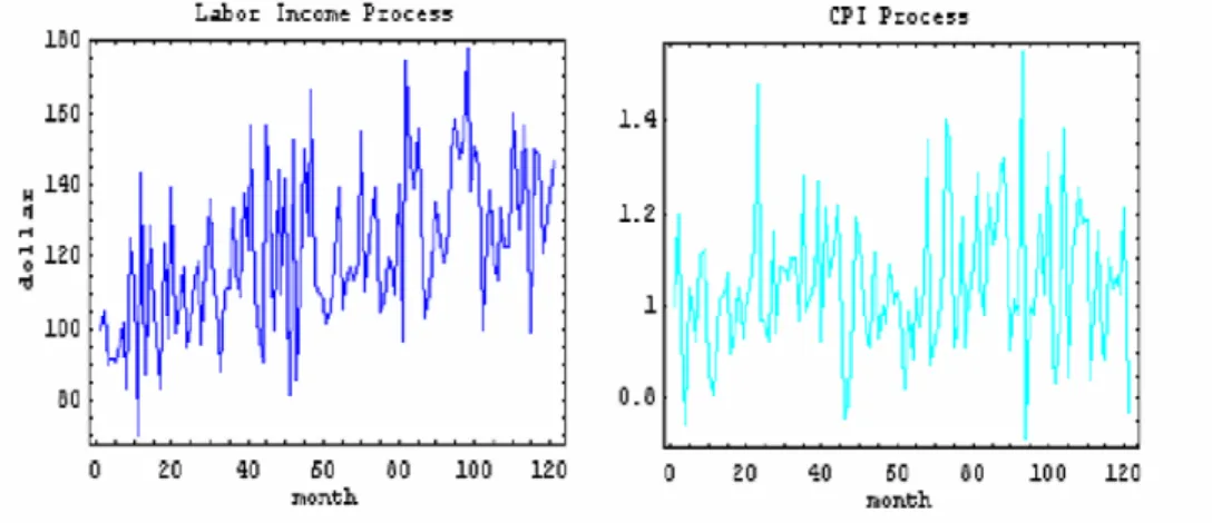
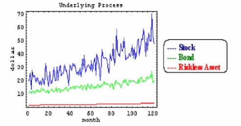
To provide the calculations of labor income and CPI effects on the optimal choice, the increase rate of labor income and rate of inflations are simulated in Figure 4. Figure 5 plots the simulated market values of the cash, the stock index and the bond funds over the investment horizon.

Figure 5 Dynamic Processes of the Underlying Assets

Figure 6 Proportion Compositions of Optimal Portfolio and Real Wealth

Figure 6 plots the optimal portfolio holdings of cash, stock and nominal bonds as a function of investment of horizon, i.e., 120 months, for an investment. The real fund wealth is also plotted for comparison.

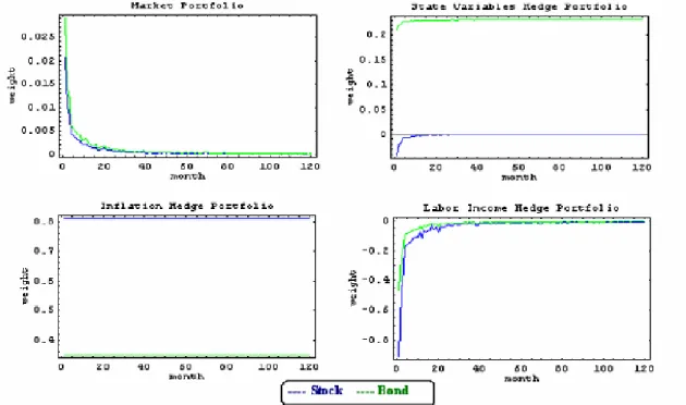
Figure 7 confirms the separation of four fund effects in the optimal portfolio selection and their behaviors in each component over time. The market portfolio has shown a decreasing trend for stock index and bond fund holdings due to the utility maximization principle. In contrast the state variable hedge portfolio shows a steady pattern for the optimal weight for bond fund and stock index holdings. To hedge the risk from the state variables, the investment strategy needs to hold a fixed proportion of bond fund and also reduce the holding of the stock index. In the inflation hedge portfolio, the investors are required to hold a high proportion of the stock index, up to 80%, to hedge the inflation risks, while only a small proportion of bond fund is sufficient in the hedge portfolio. However, in the labor income hedge portfolio, the investor should short sell

his stock index and the bond portfolio in order to preserve the salary uncertainty over his investment horizon.

Figure 7 Percentage Composition of Optimal Separated Portfolio

In Figure 8, the weights of the stock index in the entire optimal portfolio and the weights for the separated mutual funds are shown as illustration. The results indicate that the inflation hedge portfolio constitute the overwhelming proportion (75%) of the optimal portfolios. While, the state variable hedge portfolio, the market myopic portfolio and labor income hedge portfolio play only minor parts in the optimal portfolio selection problem.

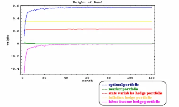
The weights of the bond fund in the entire optimal portfolio and the weights for the separated mutual funds are shown in Figure 9. These results indicate that the inflation hedge portfolio (around 35%) and the state variable hedge portfolio (around 20%) constitute the largest proportions of all long-term financial portfolios. However, the market myopic portfolio and labor income hedge portfolio play only minor parts in the optimal portfolio selection problem. Further work is required to asses more precisely the dynamics of the optimal portfolio under several plausible scenarios.

Figure 9 Proportion of Bond in the Optimal Separated Portfolio

5. Conclusion

In this paper, we investigate the asset allocation problem for defined contribution pension fund which considers not only the market risk and interest risk but also the uncertainties from labor incomes, the inflation risk and the management charges. We find that if the pension fund is to maximize the expected exponential utility of its terminal wealth, then there should be five components in its optimal asset allocation. Therefore, the optimal investment behaviors of the pension fund managers are characterized through the relative weights among the separated mutual funds according to their preference, financial market and the influential factors.

In this study, we investigate the optimal asset allocation problem incorporating both the financial and background risks. Pension fund managers must consider the short-term fund performance and the hedge requirements simultaneously. Since there exists background risks that cannot be controlled by the fund managers, a comprehensive dynamic framework is formulated to describe the decision-making process. As our results show, the dynamic portfolio that maximizes the expected utility of the plan participant consists of five components: the market portfolio, the state variables hedge portfolio, the inflation hedge portfolio, the salary uncertainty hedge portfolio and the riskless asset. By explicitly solving the optimal portfolio problem, the numerical results indicate that the inflation hedge portfolio constitutes the overwhelming proportion of stock in the optimal portfolios. In addition, the inflation hedge portfolio and the state variable hedge portfolio constitute the over-whelming proportions of bond holdings. This shows that long-term investors should hedge inflation rate risk by holding the stock index. In addition, these investors should respond to the inter-temporal hedging demands in the financial markets by increasing the average allocation to their bond fund.

To understand the roles of these components, it is necessary to explore the economic interpretations by solving the dynamic optimization problems. With respect to the most common

approach used in the literature, the incorporation of the labor income and inflation risks allows us to characterize the general pattern of the optimal strategy.

6. Appendix A

Following the work in Battocchio and Menoncin (2002), the inflation rates can be considered as a background risk affecting only the wealth growth rate, without altering the amount of wealth that can be invested. Actually, fund managers must invest the nominal fund, even though they are interested in maximizing the growth rate of the real fund. Then, we have to consider two different measures for the same fund. In particular, we call F the nominal fund _N

and F the real fund.

To model how the real fund behaves; a commonly used approximation is the following: the growth rate of the real fund is given by the difference between the nominal fund growth rate and the consumption price growth rate. If we call P the level of consumption prices, then we can write: . P dP F dF F dF N N − ≅

This is the so called Fisher equation but it gives a log-approximation of the exact relation which must hold between F and F . Actually, the true relation comes from an arbitrage _N

hypothesis. Considering the inflation rate in this framework means considering a possible arbitrage between the financial and the real market. In fact, the nominal interest rate must compensate the opportunity cost of investing in financial assets. The investor who puts his money in the financial market misses the return he could have obtained from a real investment. If the investor buys today a real good and sells it after one period, he gains the inflation rate. If he buys today a financial asset and sells it after one period, he gains a nominal return. Now, we suppose that a particular market, called the real-financial market, exists. If this is the case, then the corresponding “real-financial” return must be such that the investor is indifferent between the two following opportunities:

1. investing one nominal monetary unit in the financial market and missing the return he could have obtained on the real market;

2. investing one nominal monetary unit in the real-financial market.

Accordingly, if we call φ the real-financial return, φ_N the nominal financial return, and π the inflation rate, then the true equation that must hold between the nominal and the real fund is as follows: , π φ φ = FN ⋅ N −FN ⋅ F

which means that the return on the real wealth must equate the return on the nominal wealth reduced by the loss due to the increase in the price level. By definition it must be true that:

, , , P dP F dF F dF N N N ≡ ≡ ≡ φ π φ

and so, after substituting in the arbitrage condition, we can write: .

dP F dF dF = −